Relaxational Modes and Aging in the Glauber Dynamics of
the Sherrington-Kirkpatrick Model

1 Introduction

The fascinating features of aging effects of spin-glasses revealed by experiments [1] have arose much theoretical interest in recent years, which includes various phenomenologies [2][3], analytic predictions [4] and numerical simulations.[5][6] In order to seek for concrete information to provide theoretical base, we study the relaxational modes of the Glauber dynamics of the mean-field spin-glass model, namely Sherrington-Kirkpatrick (SK) model [7] of finite sizes at temperatures below $T_{\rm c}$ (spin-glass transition temperature). By numerically diagonalizing the transition matrix of small system sizes, we obtain a spectrum of relaxational modes and analyze their properties to get insight into the mechanism of the aging process. We also discuss the data of Monte Carlo simulations we have performed on larger system sizes.

2 Model

We study the SK model, whose Hamiltonian is given as,

$${\cal H}=\sum_{ij}J_{ij}\sigma_{i}\sigma_{j}-h\sum_{i}\sigma_{i}.$$ (2.1)

where $\sigma_{i}$’s are Ising spins, $\{J_{ij}\}$ are independent random Gaussian variables with zero mean and the variance $(N-1)^{-1}$ and $h$ is the external magnetic field.

We denote the probability that a spin configuration $\{\sigma^{\alpha}_{i}\}$ is realized at time $t$ as $p_{\alpha}(t)$. The time evolution of the probability ${\bf p}(t)=(p_{1}(t),p_{2}(t),\ldots,p_{2^{N}}(t))$, is detemined by the master equation,

$$\frac{d}{dt}{\bf p}(t)=-{\bf\mathchar 28928\relax}{\bf p}(t)\mbox{\hskip 28.45274pt with $-{\bf\mathchar 28928\relax}_{\alpha\beta}={\bf W}_{\alpha\beta}-\delta_{\alpha\beta}\sum_{\gamma}{\bf W}_{\gamma\beta}$}.$$ (2.2)

The transition probability ${\bf W}_{\alpha\beta}$ is chosen as the heat-bath type, ${\bf W}_{\alpha\beta}=\frac{1}{2}(1-\sigma_{i}^{\beta}\tanh(T^{-1}(\sum_{j}J_{ij}\sigma_{j}^{\beta}+h)))$. The unit of time corresponds with 1 Monte Carlo step/spin (MCS) used in the standard Monte Carlo simulations.

As usually done, it is convenient to introduce a matrix $\tilde{\mathchar 28928\relax}_{\alpha\beta}$ defined through the similarity transformation ${\bf\mathchar 28928\relax}_{\alpha\beta}={\bf P}_{\rm eq}^{-1/2}{\bf\tilde{\mathchar 28928\relax}_{\alpha\beta}}{\bf P}_{\rm eq}^{1/2}$. The matrix $\tilde{\mathchar 28928\relax}_{\alpha\beta}$ is a real-symmetric matrix and can be diagonalized as ${\bf\tilde{\mathchar 28928\relax}_{\alpha\beta}}=\sum_{l=1}^{2^{N}}u_{\alpha}(l)z(l)u_{\beta}(l)$ where $u_{\alpha}(l)$ is the $\alpha$-th element of the ortho-normal eigen-vector corresponding to the eigen-valuse $z(l)$. We label the eigen-values in the order $0=z(1)<z(2)<\ldots z(2^{N})$. The first mode corrsponds with the equilibrium distribution and the eigen-vector is known exactly as $u_{\alpha}(1)=\sqrt{p^{\rm eq}_{\alpha}}$. In our analysis, we perform numerical diagnalization (Householder method) to obtain the whole eigen-modes of system sizes $N=8,\ldots,12$.

Once the eigen-modes are obtained, ${\bf G}_{\alpha\beta}(t)$, the transition probability to go from $\beta$ to $\alpha$ in time $t$, can be wirtten as

$${\bf G}_{\alpha\beta}(t)=p^{\rm eq}_{\alpha}\sum_{l=1}^{2^{N}}r_{\alpha}(l)\exp(-z(l)t)r_{\beta}(l)\mbox{\hskip 28.45274pt with $r_{\alpha}(l)\equiv u_{\alpha}(l)/\sqrt{p^{\rm eq}_{\alpha}}$}.$$ (2.3)

3 Analysis

3.1. Aging after Temperature Quench

Now we consider aging process after rapid temeprature quench from the infinitely high temperature down to a temperature below $T_{\rm c}$. For this purpose, we choose the initial condition for the master equation as $p_{\alpha}(0)=1/2^{N}$, which means we choose the initial spin configuration at random. Then the system ages as

$$p_{\alpha}(t_{\rm w})=\sum_{\beta}{\bf G}_{\alpha\beta}(t_{\rm w})p_{\beta}(0).$$ (3.1)

by the propagator ${\bf G}_{\alpha\beta}(t_{\rm w})$ of a certain temperature $T<T_{\rm c}$.

In order to measure the extent to which the system approachs the equilibrium with a given $t_{\rm w}$, it is convenient to introduce the following indicator of aging,

$$R_{\alpha}(t_{\rm w})\equiv p_{\alpha}(t_{\rm w})/p^{\rm eq}_{\alpha}=\sum_{l}r_{\alpha}(l)\exp(-z(l)t_{\rm w})\sum_{\beta}r_{\beta}(l)p_{\beta}(0).$$ (3.2)

In Fig. 1 we plot an example of the evolution of the indicators at spin configurations of different energy minima. Suppose that the indicators of a pair of spin-configurations, say $\alpha$ and $\beta$, satisfy the equality with certain characteristic time $t^{*}_{\alpha\beta}$;

$$R_{\alpha}(t_{\rm w})=R_{\beta}(t_{\rm w})\mbox{\hskip 56.9055ptfor $t_{\rm w}\gg t^{*}_{\alpha\beta}$}.$$ (3.3)

Then we say that the two configurations are in quasi-equilibrium, because the relative probability that they are realized at $t_{\rm w}\gg t^{*}_{\alpha\beta}$ is the same as in the true equilibrium. In terms of eigen-modes, the above equality is equlivalent to the following one: with $l^{*}_{\alpha\beta}$ defined such that with $z(l^{*}_{\alpha\beta})\simeq(t^{*}_{\alpha\beta})^{-1}$,

$$r_{\alpha}(l)=r_{\beta}(l)\mbox{\hskip 85.35826ptfor $1\leq l\leq l^{*}_{\alpha\beta}$}.$$ (3.4)

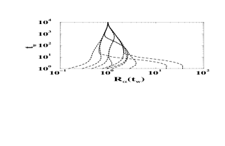
Fig. 1: The evolution of the indicator $R_{\alpha}(t_{\rm w})$ for different energy minima $\alpha$. This is an example of $N=8$, $T=0.2$ and $h=0.05$.

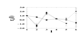
Fig. 2: The factor $\tilde{r}_{\cal B}(l)$ for different basins (different symbols) around the 6 energy minima of the system shown in Fig. 1. The error bars represent the scatterings.

3.2. Slow Modes and Hierarchical Organization of Quasi-Equlibrium Domains

Let us now introduce what we call slow modes. There are a group of the eigen-modes belonging to eigen-values $0=z(1)<z(2)<\ldots z(l_{\rm th})$ with a threshould value $l_{\rm th}$ such that the maxima of their eigen-vectors locate at the elements corresponding to the energy minima. We call this set of eigen-modes as slow modes.

For the slow modes, we have found that equality (3.4) is satisfied within each basin ${\cal B}$, the neighbourhood of an energy minimum in the phase-space, as

$$r_{\alpha}(l)\simeq\tilde{r}_{\cal B}(l)e^{\delta_{\alpha}(l)}\mbox{\hskip 14.22636ptfor $1<l<l_{\rm th}$ and $\alpha\in\cal{B}$}$$ (3.5)

up to some small scattering factors $e^{\delta_{\alpha}(l)}$. In practice, we defined the basin as a set of spin-configurations such that $T=0$ dynamics starting from any one of it converge to the energy minimum with probability one. Then we obtained $\tilde{r}_{\cal B}(l)$ and the scattering $e^{\delta_{\alpha}}$ by a $\chi^{2}$-fitting method.

The above result means that quasi-equilibrium within each basin is established at time scales specified by the slow modes. For instance, we found that the relaxation time of the $l_{\rm th}$-th mode, which is $z(l_{\rm th})^{-1}$, is about 6 MCS at $T=0.2$ independent of the system sizes we studied ($N=8,\ldots,12$). On the other hand, the relaxation time of the second mode, which is responsible for the time-reversal symmetry-breaking, grows exponentially fast with $N$, as found previously [8].

The apparent tree structure recognized in Fig. 1, is due to the follwoing. For the factor $\tilde{r}_{{\cal B}}$ of a pair of basins, say ${\cal B}_{1}$ and ${\cal B}_{2}$, there is a characteristic mode $l^{*}_{{\cal B}_{1}{\cal B}_{2}}$ such that the equality,

$$\tilde{r}_{{\cal B}_{1}}(l)=\tilde{r}_{{\cal B}_{2}}(l)\mbox{\hskip 85.35826ptfor $1\leq l\leq l^{*}_{{\cal B}_{1}{\cal B}_{2}}$},$$ (3.6)

holds within accuracy of the factor $e^{\delta_{\alpha}(l)}$ defined above, as shown in Fig. 2. The latter means that for $t_{\rm w}\gg z^{-1}(l^{*}_{{\cal B}_{1}{\cal B}_{2}})$, the two basins are in quasi-equilibrium. Thus more and more basins become in quasi-equilibrium with each other as $t_{\rm w}$ increase.

Let us call the grounp of basins, which are in quasi-equilibrium with each other at a given $t_{\rm w}$, as a quasi-equilibrium domain of age $t_{\rm w}$. To characterize the growth of quasi-equlibrium domain, we measured $d_{\rm max}(t_{\rm w})$ which is the maximum of the Hamming distance between pairs of energy minima enclosed in a domain of age $t_{\rm w}$. We found that it is an increasing function of $t_{\rm w}$.

3.3. Aging and response to magnetic field

Lastly, we present a result of our Monte Carlo simulations [9] performed on larger system sizes (but with $J_{ij}=\pm(N-1)^{-1/2}$) simulating the following well known experimental procedure [1]. For time $t_{\rm w}$ after the temperature quench, the system evolves (ages) under zero external magnetic field. Then small magnetic field $h$ is swithched on (at $t=0$) and the induced magnetization $m(t;t_{\rm w})$ is observed. We also measure the spin auto-correlation under zero-magnetic field, which is represented, by means of the notation in the previous sections, as $q(t+t_{\rm w},t_{\rm w})\equiv N^{-1}\sum_{i=1}^{N}\sigma^{\alpha}_{i}\sigma^{\beta}_{i}p^{\alpha}(t+t_{\rm w})p^{\beta}(t_{\rm w})$.

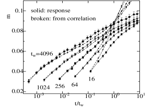
Fig. 3: Response to magnetic field and FDT

 

In Fig. 3 we plot the data of $m(t;t_{\rm w})$ and $h[1-q(t+t_{\rm w},t_{\rm w})]/T$ for $N=512$, $T=0.4$ and $h=0.1$ against $t/t_{\rm w}$. Interestingly, the two quantities coincide with each other, or satisfy the flucuation-dissipaton theorm (FDT), in the time region $t\ll t_{\rm w}$. The theorem can only be proven theoretically assuming the true equilibrium situation and the above feature seems highly non-trival. At present, we speculate that the quasi-equilibrium property we discussed before is responsible for this: at $t\ll t_{\rm w}$ fluctuation and dissipation in the system are dominated by those in the quasi-equilibrium domain of age $t_{\rm w}$, while at later $t$ the system starts to invade a bigger domain which causes the breaking of the FDT.

To summarize, we have studied the relaxational modes and aging of the SK model by numerical diagonalization technique and Monte Carlo simulations. We focused on the charcteristics of the slow modes and found that the aging proceed by hierarchical growth of quasi-equilibrium domains.

The numerical works have been done on FACOM VPP-500/40 at the Super Computor Center, Institute for Solid State Physics, University of Tokyo. This work was supported by Grand-in-Aid for Scientific Research from the Ministry of Education, Science and Culture, Japan. One of the author (HY) was supported by Fellowships of the Japan Society for the Promotion of Science for Japanese Junior Scientists.

References

• [1] For a review, see E.Β Vincent, J.Β Hammann and M.Β Ocio, in Recent Progress in Random Magnets (World Scientific, Singapore, 1992).
• [2] J.Β P.Β Bouchaud, J. Phys. (France) 2 (1992) 1705.
• [3] R. G. Palmer 1982, Adv. In. Phys. vol. 31 669, P. Sibani and K. H. Hoffmann 1989, Phys.Β Rev.Β Lett.Β 63 2853, H. Yoshino 1996, J.Β Phys. A (to be published) cond-mat/9604033.
• [4] L.Β F.Β Cugliandolo and J.Β Kurchan, J.Β Phys. A 27 (1994) 5749.
• [5] L.Β F.Β Cugliandolo, J.Β Kurchan and F.Β Ritort, Phys.Β Rev. B 49 (1994) 6331,
• [6] A. Baldassarri, preprint, cond-mat/9607162.
• [7] D.Β Sherrington and S.Β Kirkpatrick, Phys.Β Rev.Β Lett. 35 (1975) 1792.
• [8] A.Β P.Β Young and S.Β Kirkpatrick, Phys.Β Rev. B 25 (1981) 440.
• [9] H.Β Takayama, H.Β Yoshino and K.Β Hukushima, preprint cond-mat/9612071