Coherent noise, scale invariance and intermittency
in large systems

Abstract

We introduce a new class of models in which a large number of “agents” organize under the influence of an externally imposed coherent noise. The model shows reorganization events whose size distribution closely follows a power-law over many decades, even in the case where the agents do not interact with each other. In addition the system displays “aftershock” events in which large disturbances are followed by a string of others at times which are distributed according to a $t^{-1}$ law. We also find that the lifetimes of the agents in the system possess a power-law distribution. We explain all of these results using an approximate analytic treatment of the dynamics and discuss a number of variations on the basic model relevant to the study of particular physical systems.

and

1 Introduction

There has in the past few years been considerable interest across a broad section of the scientific community in extended dynamical systems which show intermittent events or “avalanches” of activity whose size follows a power-law frequency distribution. Examples of such systems include earthquakes [1, 2, 3, 4], solar flares [5], avalanches [6] and laboratory experiments on stick slip dynamics [7]. Behaviour of this type presents something of a puzzle; the central limit theorem tells us that scale-free behaviour should not exist in a system of independent agents unless the behaviour of the individual agents is itself scale-free, which in general it is not. The introduction of interactions between the agents does not necessarily alleviate the problem either. It is well known, for instance, that scale-free fluctuation distributions occur in interacting systems close to continuous phase transitions. But such systems require careful tuning of their parameters to bring them to criticality, whereas experiments such as those mentioned above appear to be very robust against parameter changes.

One resolution of this difficulty was proposed by Bak, Tang and Wiesenfeld [8] who in 1987 introduced the idea of the self-organized critical (SOC) system. In this paper the authors proposed that, under the action of a slow local driving force, certain systems possessing only short-range interactions can organize themselves into a critical state, without the need for any parameter tuning. Once a system organizes itself in this way, all the familiar arguments concerning critical phenomena can be brought to bear, including the crucial concept of universality and the robustness which it implies. The universal properties of critical systems, including such measurable quantities as the exponents of power-law distributions, should be robust against changes in the microscopic dynamics of the system; if the differences between the true physical system—tectonic fault, sandpile or solar corona—and the simple SOC model system can be shown (or assumed) to reside entirely in the irrelevant variables, then the model provides not only a qualitative description of the dynamics, but also a quantitative method for calculating the universal properties.

The original model of Bak et al. was a simple representation of the dynamics of avalanches, but many other SOC models have been proposed since, as models of a wide variety of physical phenomena. Perhaps the simplest such model is the “minimal SOC model” of Bak and Sneppen [9], originally constructed as a model of coevolutionary avalanches in large ecosystems, although Ito [10] has suggested that it might also find use as a model of earthquake dynamics. A number of other SOC models of earthquakes have also been proposed, including de Sousa’s “train” version of the sliding-block model of Burridge and Knopoff [11, 12], as well as related models put forward by various authors [13, 14, 15, 16, 17, 18]. Other applications of the self-organized criticality idea include the modelling of forest fires [19, 20] and the mathematically similar problem of predator-prey interactions in spatially extended ecosystems [21], the dynamics of solar flare generation [22, 23], interface depinning [24, 25], and a variety of other phenomena (see the review by Paczuski, Maslov and Bak [26]).

However, we must also be cautious in interpreting the observation of power-law distributions in experimental systems as evidence of SOC behaviour. There are many other possible explanations of how such a power-law distribution might arise: random multiplicative processes [27], thermal crossing times for random barriers [28], fragmentation processes [29, 30], and a number of other common physical processes give rise to power-law distributions. One could justifiably argue that mechanisms such as these are less flexible than SOC models, and therefore have less power as explanations of physical phenomena. Many of them for example can only produce one particular value of the exponent of a power law, whereas both SOC models and the experiments they attempt to model can show a variety of exponent values. However, SOC models have their limitations too. Many SOC models, including the minimal model of Bak and Sneppen, can be mapped in the limit of infinite dimension onto a critical branching process, which allows us to relate the exponent describing the fluctuation distribution to the first return time of a one-dimensional random walk [9]. The result is that we expect these models to possess an event size distribution characterized by an exponent of value ${\textstyle\frac{3}{2}}$ for all dimensions above some upper critical dimension, and lower exponent values for dimensions below this. Unfortunately, a number of systems for which SOC models have been proposed display distributions with steeper exponents than this. The distribution of the areas of terrestrial earthquakes for example appears to follow a power-law with exponent $2.0\pm 0.1$ [1, 2], and the laboratory experiments on avalanches in rice-piles conducted by Frette et al. [6] show an exponent of $2.1\pm 0.1$.

In this paper we discuss a new class of models which are not critical models, but which nonetheless display a power-law distribution of event sizes, robust against virtually any change in the microscopic dynamics of the system. The exponent of the power-law can take a range of values, although for most plausible choices of the parameters of the model its value lies in the range $2.0\pm 0.2$. The dynamics of our models is fundamentally different from that of SOC models, being driven not by a slow, local driving force, but by a coherent, externally-imposed noise term. Our models do not display long-range spatial correlation or critical fluctuations and hence possess spatial configurations at equilibrium which are qualitatively entirely different from SOC models. It is our suggestion that some of the systems traditionally studied using SOC models might in fact be coherent-noise driven systems of the type described in this paper.

One simple example of a coherent-noise driven model displaying robust power-law distributions has already been presented elsewhere [32]. In that paper we discussed the use of this model as a model of sandpile dynamics and also of earthquakes. Newman [33] has also employed a variation of the model to study the distribution of event sizes in biological extinction, another example of a system which appears to have a power-law distribution too steep to be easily explained using SOC dynamics. In this paper we will concentrate primarily on the analysis of our models, demonstrating the origin and limits of the power-law distributions and their robustness. The outline of the paper is as follows. In Section 2 we introduce the simplest class of models displaying the phenomena of interest. In Section 3 we present numerical results of the simulation of a large number of members of the class, displaying explicitly the robustness of properties across the spectrum of parameter values, as well as the limits of that robustness. In Sections 4 and 5 we give a detailed analysis of these models. In Sections 6 and 7 we discuss our results and give our conclusions.

2 The model

Consider a system composed of $N$ “agents”. In SOC models these agents might be grains of sand in a sandpile, or species in an evolving ecosystem. These agents are subject to “stresses” $\eta(t)$ at each time-step $t$, chosen at random from some probability distribution $p_{\rm stress}(\eta)$. Each agent $i$ possesses a “threshold” $x_{i}$ of tolerance for these stresses, chosen from another distribution $p_{\rm thresh}(x)$. If the stress level at any time exceeds an agent’s threshold value, then that agent “moves”, or “dies out”, and its threshold $x_{i}$ is given a new value, chosen from the same distribution. Thus, over time, the stresses on the system will tend to remove low threshold values from the system and replace them with higher ones. Assuming that the distribution $p_{\rm stress}(\eta)$ has a well-defined mean, this means that the system will eventually stagnate, when we get to the point where all the thresholds are well in excess of that mean and there are none left within reach of the typical stresses. In order to prevent this happening, we add a second element to the dynamics, an “aging” or “reloading” process in which at every time-step a certain small fraction $f$ of the agents, chosen at random regardless of their thresholds, are given new values of $x_{i}$, chosen from the same distribution as before. The dynamics of the model can thus be summarized as follows:

1. At each time-step a stress level $\eta$ is chosen at random from a distribution $p_{\rm stress}(\eta)$ and all agents with thresholds $x_{i}<\eta$ move and are given new threshold values chosen from a distribution $p_{\rm thresh}(x)$. The number of agents which move is the size of the event taking place in this time-step.

2. A small fraction $f$ of the agents are chosen at random from the population and given new thresholds, also chosen from the distribution $p_{\rm thresh}(x)$.

A few points to notice about this model:

At least in this simplest version of the model the agents are entirely non-interacting. We have investigated other variants in which the agents are allowed to interact (see Section 6), but the basic predictions of the model are unchanged.

The dynamics is fundamentally a competition between the two processes. The first tends to remove from the system agents with low thresholds for stress. This means that the distribution of thresholds tends to be weighted towards high values of $x_{i}$. This in turn means that the second process, which selects agents without regard to their threshold values, is more likely to pick ones with high $x_{i}$ and therefore will on average tend to reduce the mean threshold value of the population.

The basic parameters of the system are the two distributions $p_{\rm stress}$ and $p_{\rm thresh}$, and the aging parameter $f$. We have not chosen precise values of these parameters here, and one feels intuitively that the behaviour of the model should depend on what choice we make. In general, this is a correct intuition. However—and this is our main point—it turns out that some of the most striking properties of this model and its variants are independent of our choice over a very large range of possibilities. In the case of the variable $f$ all that we will require is that its value be small, but non-zero, in a way which we will make precise in Section 4. The conditions on $p_{\rm stress}$ and $p_{\rm thresh}$ are more subtle, but, as we shall see, are relaxed enough that virtually any distribution of stresses one might expect to encounter in a real system is included.

In the next section we illustrate the basic properties of the model using the results of numerical simulations.

3 Numerical results

The most striking property of the class of models we have described is that the distribution of the sizes of the events taking place follows a power-law closely over many decades for most reasonable choices of $p_{\rm stress}$ and $p_{\rm thresh}$. First of all, let us consider the case where $p_{\rm thresh}(x)$ is 1 if $0\leq x<1$ and zero otherwise. In other words, the thresholds are chosen uniformly in the interval between zero and one. This particular choice has the advantage that the model can be simulated in the limit $N=\infty$ using a fast algorithm we have developed which acts directly on the distribution $\rho(x)$ of thresholds, rather than on the individual agents themselves. Figure 1 shows the results of such simulations for a variety of choices of the stress distribution, including Poissonian noise, Gaussian noise, stretched exponentials, and power laws. Note that in each case, the distribution of event sizes follows a power law over a large part of its range, deviating only at very low event sizes.

Figure 1: The distribution of event sizes for the model with $p_{\rm thresh}(x)$ uniform and a variety of choices for the imposed stress distribution. The stress distributions correspond to those of Table 1 as follows: (i) steep, (ii) Gaussian (c), (iii) Gaussian (b), (iv) Gaussian (a), (v) Poissonian, (vi) exponential, (vii) stretched (a), (viii) stretched (b) and (ix) Lorentzian. The aging parameter $f=10^{-6}$ in each case. The curves have been rescaled so as not to overlap.

In Table 1 we give the measured exponent $\tau$ of these power-law distributions, and, as the table makes clear, the exponent varies depending on the distribution of the noise. The values are all in the vicinity of $\tau=2$, though for very slowly-decaying noise distributions they get closer to one. Notice however that for systems driven by noise with the same distribution but different values of the scale parameter $\sigma$ (e.g., the width of the Gaussian for Gaussian noise) the value of $\tau$ is the same. Furthermore, noise distributions with the same functional form in their large $\eta$ tail, such as the Gaussians centered at zero and at ${\textstyle\frac{1}{2}}$, also give the same values of $\tau$.

noise type	$p_{\rm stress}(\eta)$	exponent $\tau$
steep	$\exp(-\eta^{4}/\sigma^{4})$	$2.22\pm 0.06$
Gaussian (a)	$\exp(-\eta^{2}/2\sigma^{2})$ with $\sigma=0.05$	$2.01\pm 0.02$
Gaussian (b)	$\exp(-\eta^{2}/2\sigma^{2})$ with $\sigma=0.1$	$2.04\pm 0.02$
Gaussian (c)	${\textstyle\frac{1}{2}}+\exp(-\eta^{2}/2\sigma^{2})$	$2.04\pm 0.04$
Poissonian	$\mu^{\eta/\sigma}/\Gamma(\eta/\sigma+1)$	$1.97\pm 0.03$
exponential	$\exp(-\eta/\sigma)$	$1.85\pm 0.03$
stretched (a)	$\exp[-(\eta/\sigma)^{0.5}]$	$1.76\pm 0.04$
stretched (b)	$\exp[-(\eta/\sigma)^{0.2}]$	$1.32\pm 0.02$
Lorentzian	$(\sigma^{2}+\eta^{2})^{-1}$	$1.30\pm 0.08$

Table 1: Definition of the various noise distributions used in Figure 1, along with the measured value of the event size exponent $\tau$ for each case.

In Figure 2 we show the results of a set of simulations for systems with the same Gaussian noise distribution, but different values of the aging parameter $f$. As the figure shows, varying $f$ varies the size of the region over which power-law behaviour is seen, but again, does not vary the exponent of the power-law.

Figure 2: The distribution of event sizes for the model with a Gaussian stress distribution of mean zero and width $\sigma=0.05$, with values for the aging parameter $f$ varying from $10^{-6}$ (lowest curve) to $10^{-2}$ (highest).

In Figure 3 we show results for simulations performed with choices of $p_{\rm thresh}$ different from the uniform one used above. In this case we chose both $p_{\rm thresh}$ and $p_{\rm stress}$ to be exponentials, and held the decay parameter $\sigma$ for $p_{\rm stress}$ fixed whilst varying that for $p_{\rm thresh}$. As long as the fall-off in $p_{\rm thresh}$ is slower than that for $p_{\rm stress}$, we continue to see power-law behaviour. But once $p_{\rm thresh}$ starts to fall off faster, the power-law is destroyed. (Note that these simulations were, necessarily, performed for finite $N$, using a slower algorithm than the previous figures, so the statistics are poorer.)

Figure 3: The distribution of event sizes for the model with stresses distributed exponentially (see Table 1) with $\sigma$ held fixed at $0.05$ and an aging parameter $f=10^{-6}$. The different curves correspond to different choices of the distribution $p_{\rm thresh}(x)$ from which the thresholds are selected. In this case $p_{\rm thresh}(x)$ was also an exponential distribution with decay constants (left to right) of $0.5$, $0.2$, $0.1$ and $0.05$. The power-law form is maintained until the decay constant becomes extremely short.

In Figure 4 we show the distribution of events for a system in which the stresses were chosen uniformly in the interval between zero and one, just as were the thresholds. Clearly, this choice does not result in a power-law distribution of event sizes.

Figure 4: The distribution of event sizes for a simulation in which both the thresholds and the stress levels were chosen uniformly in the interval between zero and one. Clearly this distribution does not obey a power law.

In Section 4 we offer theoretical arguments in explanation of each of these phenomena.

There are a number of other interesting features to be seen in the behaviour of these models. In Figure 5, we show the distribution of the “lifetimes” of agents in the model—the number of time-steps between one move and the next of a particular agent. This too is a power-law, with an exponent close to $1$ in the case of the exponential stress distribution employed here. (Another measure of the time behaviour of the system is the power spectrum of the pattern of activity. However, this spectrum turns out to go like $1/f^{2}$, a form seen in such a wide variety of dynamical systems that it tells us very little about the properties of the model.)

Figure 5: The distribution of lifetimes of agents in a simulation with exponential stresses. The distribution is a power law with an exponent of $1.00\pm 0.02$.

A feature of these models which may prove useful in distinguishing the present dynamics from SOC systems is the existence of “aftershocks”—large events following closely on the tail of others. Figure 6 shows a sample of time-series data from one of our simulations displaying a set of aftershocks. In Figure 7 we have measured the time-delay between a large event and each of the succeeding aftershocks. A histogram of these time delays shows a $t^{-1}$ functional form. Interestingly the exponent here seems to be independent of the nature of the stresses driving the system.

Figure 6: A section of the time-series of reorganization events in a simulation of the model. The aftershocks following the first large event are clearly visible. Notice also that some of the aftershocks themselves generate a smaller series of after-aftershocks.

Figure 7: A histogram of the time distribution of aftershocks following a large event. The distribution follows a power law with an exponent very close to one.

4 Analysis

As we saw in the last section, models of the type discussed here generate scale-free distributions of a number of measurable quantities, including the sizes of the reorganization events. These distributions are robust against most changes we can make in the parameters of the models, and for this reason we believe that models of this type may provide an explanation for the characteristic fluctuation distributions and intermittency seen in a number of extended dynamical systems. As Figures 3 and 4 show however, there are limits to the robustness of the various distributions, as well as some qualitative differences between these models and the SOC models (such as the aftershocks depicted in Figure 6). In this section we develop a theoretical picture of the behaviour of our models, demonstrate the causes of the robustness and the reasons why it breaks down in some cases, and give quantitative explanations of the existence and distribution of aftershocks, agent lifetimes, and other features of these systems.

First, we note that it is a straightforward matter to solve for the mean (i.e., time-averaged) distribution $\bar{\rho}(x)$ of the threshold variables $x_{i}$. In any small interval $\d x$, the rate at which agents leave the interval because of the aging process is $f\bar{\rho}(x)\>\d x$. In the same interval the probability per unit time $p_{\rm move}(x)$ of an agent being hit by a stress event is simply the probability that the stress level $\eta$ will be greater than $x$ in that time-step, which is

$$p_{\rm move}(x)=\int_{x}^{\infty}p_{\rm stress}(\eta)\>\d\eta.$$ (1)

The mean rate at which agents in the interval get hit by the stress events is therefore equal to $p_{\rm move}(x)\>\bar{\rho}(x)\>\d x$. The rate at which the interval $\d x$ is repopulated is simply $A\>p_{\rm thresh}(x)\>\d x$, where $A$ is an $x$-independent constant whose value is equal to the total integrated rate at which agents are lost to both the aging and stress processes. Thus, we can write a master equation balancing the rates of agent loss and repopulation which should describe the time-averaged equilibrium state of the model:

$$f\bar{\rho}(x)+p_{\rm move}(x)\>\bar{\rho}(x)=A\>p_{\rm thresh}(x).$$ (2)

Rearranging for $\bar{\rho}(x)$, we get

$$\bar{\rho}(x)={A\>p_{\rm thresh}(x)\over f+p_{\rm move}(x)}.$$ (3)

This equation is exact. For any given choice of $p_{\rm thresh}(x)$ and $p_{\rm stress}(\eta)$, the constant $A$ can be fixed by requiring that $\bar{\rho}(x)$ integrate to unity over the allowed range of $x$ values.

To give a concrete example, consider the simple case where $p_{\rm thresh}(x)$ is uniformly distributed over the interval between zero and one and $p_{\rm stress}(\eta)$ is the normalized exponential distribution

$$p_{\rm stress}(\eta)=\frac{1}{\sigma}\exp(-\eta/\sigma).$$ (4)

(The stress $\eta$ is restricted to non-negative values.) In this case, $p_{\rm move}(x)=\exp(-x/\sigma)$ and so

$$\bar{\rho}(x)={A\over f+\exp(-x/\sigma)}.$$ (5)

The constant $A$ is

$$A={f\over\sigma}\biggl{[}\log{f\exp(1/\sigma)+1\over f+1}\biggr{]}^{-1}.$$ (6)

In Figure 8 we have plotted this expression for $\bar{\rho}(x)$ along with data for the same quantity from our numerical studies. The agreement between the two is excellent. Notice some crucial features of the curve. First, the probability $p_{\rm move}(x)$ that an agent with threshold $x$ will lie below the stress level on any particular time-step decreases monotonically with $x$, regardless of the form of the stress distribution. Thus, as long as $f$ is finite there will always be some value of $x$, call it $x_{c}$, above which Equation (3) is dominated by the first term in the denominator so that $\bar{\rho}(x)$ is simply proportional to $p_{\rm thresh}(x)$. Below $x_{c}$ there is a regime in which the second term dominates, making $\bar{\rho}(x)$ proportional to $p_{\rm thresh}(x)/p_{\rm move}(x)$:

$$\bar{\rho}(x)\approx{A\>p_{\rm thresh}(x)\over p_{\rm move}(x)}.$$ (7)

In the exponential example considered above this becomes

$$\bar{\rho}(x)\approx A\>\exp(x/\sigma).$$ (8)

As we will see, it is this part of the curve which is responsible for the power-law distribution of event sizes in the model. The crossover point $x_{c}$ between the two regimes is defined by

$$p_{\rm move}(x_{c})=f,$$ (9)

which means that the value of $f$ controls the range of event sizes over which we have power-law behaviour, the range increasing as $f$ gets smaller.

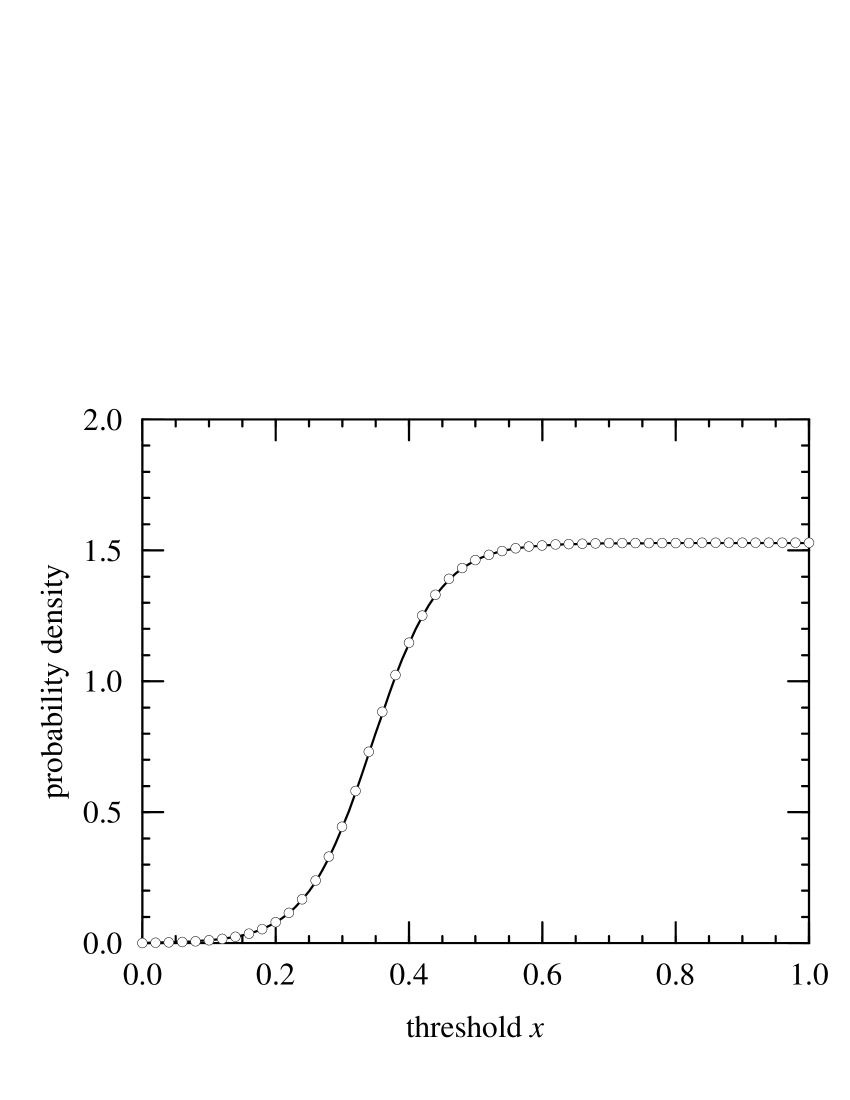
Figure 8: The average threshold distribution $\bar{\rho}(x)$ for the model with exponentially distributed stresses with $\sigma=0.05$. The solid line is the analytic expression, Equation (3), and the points are the numerical data.

The size of the event which corresponds to a stress of magnitude $\eta$ is given by

$$s(\eta)=\int_{-\infty}^{\eta}\rho(x)\>\d x.$$ (10)

In general the threshold distribution at any particular time $t$ will differ from the time-averaged distribution $\bar{\rho}(x)$. In this section however, we will make the approximation that the two are equal, which allows us to solve for the event size distribution. We will refer to this as the “time-averaged approximation” (TAA), and in practice it turns out to be a good guide to the average behaviour of the system, though there are some limitations to what it can tell us. (In particular, it can tell us nothing about time correlations in the system, and therefore cannot explain the aftershocks of Figure 6, for example.)

For thresholds distributed according to Equation (3), the probability density of events of size $s$ is given by

$$p_{\rm event}(s)=p_{\rm stress}(\eta){\d\eta\over\d s}={p_{\rm stress}(\eta(s))\over\bar{\rho}(\eta(s))},$$ (11)

where we have calculated $\d\eta\over\d s$ by substituting $\bar{\rho}(x)$ in place of $\rho(x)$ in Equation (10) and differentiating, and the function $\eta(s)$, which is the stress required to produce an event of size $s$, is given by the functional inverse of Equation (10). This function $\eta(s)$ is a monotonic increasing function of $s$, and this immediately leads us to our first result about the model: all events of size greater than a given size $s$ are produced by stresses greater than $\eta(s)$. Thus, the high-$s$ tail of the event distribution depends only on the functional form of the high-$\eta$ tail of the stress distribution. This offers an explanation (at least within the TAA) of the behaviour observed in the figures of Section 3, in which stress distributions with the same high-$\eta$ tail gave rise to event distributions obeying the same power-law.

We are also now in a position to answer the question of how the power-law distribution of events arises. As we mentioned above, the power-law depends on the low-$x$ part of the threshold distribution, the part below $x_{c}$. In this regime Equation (7) is valid and, making use of Equations (1) and (11), we write

$$p_{\rm event}(s)=A^{-1}{p_{\rm stress}(\eta(s))\int_{\eta(s)}^{\infty}p_{\rm stress}(x)\>\d x\over p_{\rm thresh}(\eta(s))},$$ (12)

Making the same approximations in Equation (10), we get

$$s(\eta)=\int_{-\infty}^{\eta}{A\>p_{\rm thresh}(x)\over\int_{x}^{\infty}p_{\rm stress}(\eta^{\prime})\>\d\eta^{\prime}}\>\d x.$$ (13)

Between them, these two equations define the event size distribution. As it turns out the form of $p_{\rm thresh}(x)$ is virtually irrelevant to the form of $p_{\rm event}(s)$, our only requirement being that it should vary relatively little between the minimum value of $x$ and the value $x_{c}$. Variation by a factor of ten or so would be acceptable. To see this we need only consider the distributions of event sizes shown in the last section: typically $p_{\rm event}(s)$ varies over many orders of magnitude, as many as twenty in some cases. Clearly then, one order of magnitude variation in the denominator of Equation (12) is not going to make much difference. It is certainly possible to arrange for $p_{\rm thresh}(x)$ to vary fast enough to destroy the power-law behaviour—just as we did in Figure 3—but for most reasonable choices the functional form is unimportant.

So what does the event distribution depend on? The crucial condition which must be fulfilled if we are to get a power-law distribution of event sizes turns out to be that the value of $p_{\rm stress}(\eta)$ in the tail should fall off fast enough that the integral of $p_{\rm stress}(\eta)$ from $\eta$ to $\infty$ should be dominated by the value of the function near $\eta$. In its most general form, this condition can be stated as:

$$\int_{\eta}^{\infty}p_{\rm stress}(x)\>\d x\sim p_{\rm stress}^{\alpha}(\eta).$$ (14)

Substituting this condition into Equations (12) and (13), and neglecting variation in $p_{\rm thresh}(x)$, we find that

$$p_{\rm event}(s)\sim p_{\rm stress}^{\alpha+1}(\eta(s)),$$ (15)

and

$$s(\eta) \sim \int_{-\infty}^{\eta}p_{\rm stress}(x)^{-\alpha}\>\d x=\int_{0}^{p_{\rm stress}(\eta)}p_{\rm stress}^{-\alpha}{\d x\over\d p_{\rm stress}}\>\d p_{\rm stress}$$ (16)

$$= {1\over p_{\rm stress}(\eta)},$$

where we have employed Equation (14) to evaluate the derivative. Now we can combine these two equations to give:

$$p_{\rm event}(s)\sim s^{-\tau},$$ (17)

where

$$\tau=\alpha+1.$$ (18)

As we will see, the value of $\alpha$ for most of the distributions $p_{\rm stress}(x)$ which we have considered is close to one, with the result that $\tau$ is usually close to two.

To make these developments a little more specific, let us look at some examples. Two cases in which Equation (14) is exactly true are the cases of stress distributions $p_{\rm stress}(\eta)$ with either an exponential or a power-law tail:

$$\int_{\eta}^{\infty}\e^{-x/\sigma}\>\d x\propto\e^{-\eta/\sigma} \alpha=1$$ , i.e.,  (19)

$$\int_{\eta}^{\infty}\Bigl{(}{x\over\sigma}\Bigr{)}^{-\gamma}\>\d x\propto\Bigl{(}{\eta\over\sigma}\Bigr{)}^{-\gamma+1} \alpha=1-\frac{1}{\gamma}$$ , i.e., . (20)

Hence, we can expect the distributions of events produced by, for example, the Poissonian and Lorentzian stress distributions to be essentially perfect power-laws. In almost all the other cases considered in the last section, the condition (14) is true to a good approximation, which explains why we still see power-law behaviour over many decades. For example, in the case of stress distributions with a Gaussian tail we have:

$$\int_{\eta}^{\infty}\exp\Bigl{(}-{x^{2}\over\sigma^{2}}\Bigr{)}\>\d x\propto\mathop{\rm erfc}(\eta/\sigma).$$ (21)

However, the error function $\mathop{\rm erfc}(x)$ has a tail which goes like $\exp(-x^{2})/x$. The $x^{-1}$ decays much slower than the Gaussian, and so to a good approximation Equation (14) still holds over any region in which $\eta$ is comparable to or greater than $\sigma$. Thus in the case of Gaussian stresses we also find a power-law distribution of event sizes. The theory outlined above predicts $\tau=2$ in both the exponential and Gaussian cases, and $\tau={\textstyle\frac{3}{2}}$ in the Lorentzian case. These figures are in moderately good agreement with measured figures of $\tau=2.0$ for the Gaussian, $\tau=1.9$ for the exponential, and $\tau=1.3$ for the Lorentzian. For most of the other cases examined in Section 3 we can also demonstrate, at least approximately, the validity of Equation (14) and deduce a value for the exponent $\tau$ which is in approximate agreement with the numerical results. The extent to which the predicted and observed exponents do not agree is a measure of the validity of the TAA; the difference between the two is presumably due to fluctuation of $\rho(x)$ around the mean distribution $\bar{\rho}(x)$.

Stress distributions which do not satisfy Equation (14), such as the flat one used in Figure 4, or indeed any distribution which does not have a tail, will not produce a power-law distribution of event sizes. However, we contend that virtually all naturally occurring stress distributions which a system is likely to encounter are covered by the many cases we have shown in Section 3, and hence that, for systems driven by coherent stress in this fashion, power-law event size distributions with exponents in the vicinity of two should be a ubiquitous phenomenon.

Now we turn our attention to the distribution of lifetimes of the agents in the model. Using the same approximations which we employed above to study the event size distribution we can show that we should also expect the lifetime distribution to follow a power law. First, note that the typical lifetime $L$ of an agent possessing a threshold value $x$ is simply related to the probability $p_{\rm move}(x)$ (Equation (1)) of it being hit by the stress on any particular time-step:

$$L={-1\over\log[1-p_{\rm move}(x)]}\approx{1\over p_{\rm move}(x)},$$ (22)

the latter equality holding when $L$ is significantly greater than one, which is the case we are interested in. We can then use this equation to relate the probability distribution of lifetimes over the population $p_{\rm pop}(L)$ to the distribution of thresholds $x$, which we approximate by its value within the TAA:

$$p_{\rm pop}(L)=\bar{\rho}(x){\d x\over\d L}.$$ (23)

Note however, that the contribution of the longer-lived agents to this distribution will be greater than that of the shorter-lived ones, in proportion to their lifetimes. It is more common to calculate the distribution of lifetimes as an average simply over all agents, a distribution which would be given by:

$$p_{\rm agents}(L)\propto\bar{\rho}(x){1\over L}{\d x\over\d L}.$$ (24)

The derivative can be evaluated using Equations (1) and (22) thus:

$${\d L\over\d x}={-1\over p_{\rm move}^{2}(x)}{\d p_{\rm move}(x)\over\d x}={p_{\rm stress}(x)\over p_{\rm move}^{2}(x)}.$$ (25)

The threshold distribution $\bar{\rho}(x)$ we get from Equation (7), assuming as we did earlier that $p_{\rm thresh}(x)$ changes little over the region of interest. Then

$$p_{\rm agents}(L)\propto{1\over L}\>{p_{\rm move}(x)\over p_{\rm stress}(x)}\sim L^{-2+\frac{1}{\alpha}},$$ (26)

where we have made use of Equation (14) again. For stress distributions such as the exponential, Poissonian and Gaussian distributions, for which $\alpha=1$, this gives a lifetime distribution which goes like $L^{-1}$, a figure which is confirmed well by the numerical data. The exponent in Figure 5, for example, is $1.00\pm 0.02$.

5 Results beyond the time-averaged approximation

One result which is clearly outside the realm of the time-averaged approximation, but which nevertheless admits of a very simple explanation, is the existence of the aftershock events seen in Figure 6, and the power-law distribution of the times at which they occur, as shown in Figure 7. The basic explanation of the existence of the aftershocks is this. When a large stress event occurs, a significant fraction of the agents in the system move, and acquire new threshold values distributed according to $p_{\rm thresh}(x)$. As we pointed out in Section 2, this typically lowers the mean threshold value, producing a distribution $\rho(x)$ with more weight at low $x$ than the average distribution $\bar{\rho}(x)$. The result is that when, some short time later, another stress of only moderate size hits the system, it will affect a larger number of agents than one would normally expect, producing an aftershock event.

As Figure 7 shows, the times $t$ after the initial large event at which aftershocks occur, are distributed according to a power law. The exponent of this distribution is one in all cases we have investigated, a finding which we explain as follows. Consider what happens when a large event takes place. Following such an event, a large fraction of the agents in the system are assigned new threshold values drawn at random from the distribution $p_{\rm thresh}(x)$. Shortly thereafter, the first aftershock event occurs, when some moderate-sized stress $\eta_{1}$ hits the system and wipes out all agents with $x<\eta_{1}$. In order to get a second aftershock we now need a larger stress $\eta_{2}$, to reach agents who were not hit during the first aftershock. If it took a time $t_{1}$ to generate a stress of size $\eta_{1}$, then it will, on average, take as long again to generate another stress of greater or equal magnitude, or an aggregate time of $t_{2}=2t_{1}$. Repeating this argument for the third aftershock we can see that it will occur an average of $t_{3}=2t_{2}$ after the initial large event, and so forth. In general the $n^{\rm th}$ aftershock will occur a time

$$t=t_{1}2^{n}$$ (27)

after the initial event. The average number of aftershocks $\d n$ occurring in an interval $\d t$ of time after the initial large event (which is what Figure 7 shows) is then

$$\d n={\d t\over t_{1}n2^{n-1}}={2\d t\over nt}.$$ (28)

From Equation (27) we can see that the $n$ in the numerator varies as $\log t$. Thus, apart from logarithmic corrections, the distribution of aftershock times goes as $t^{-1}$. This argument makes no assumptions at all about the form of $p_{\rm stress}(\eta)$ or $p_{\rm thresh}(x)$, and so can be expected to hold regardless of how we choose these functions, which is indeed what we see in our simulations.

We can also ask about the size of the aftershock events, and it turns out that there is a very simple argument giving the distribution of this quantity as well. Consider a large event which reorganizes a significant fraction $s_{0}$ of the agents in the system. The disturbed agents are redistributed according to the function $p_{\rm thresh}(x)$, which, as we have assumed, is slowly varying over the region of $x$ of interest. If our large event is followed some time later by a stress event of moderate size $\eta_{1}$, the size $s_{1}$ of the corresponding aftershock is then proportional to $s_{0}$. Given that our TAA predicts that $s_{0}$ will be distributed according to a power law, this tells us that the aftershocks must be distributed according to the same power law, even though the TAA itself can tell us nothing about the aftershocks. We can extend this argument to tell us something about the distribution $p(s|\eta)$ of event sizes $s$ produced by stresses of a certain strength $\eta$: the large-$s$ tail of $p(s|\eta)$ is presumably dominated by aftershock events since these are, on average, larger than events for the same size $\eta$ which do not occur immediately after another large event. But the distribution of aftershocks has, as we have said, a power-law form with the same exponent as the overall event size distribution, and hence we can conclude that $p(s|\eta)$ should also fall off like a power law with the same exponent. In Figure 9 we have plotted $p(s|\eta)$ for a variety of values of $\eta$ on logarithmic scales which clearly shows this power-law functional form. Within the TAA, we assume that only one size of event is produced by a given value of $\eta$ (see Equation (10)) and hence that $p(s|\eta)$ is equal to a $\delta$-function $\delta(s-s(\eta))$, but this is only an approximation. In reality, as Figure 9 shows, a stress of size $\eta$ can produce a variety of different event sizes, depending on the instantaneous distribution of thresholds, but, to the extent that this distribution is narrow and approximates well to a $\delta$-function, the TAA should be a reliable approximation.

Figure 9: A plot of the probability $p(s|\eta)$ of getting an event of size $s$ given a stress of size $\eta$. The stresses were Gaussianly distributed with mean zero and width $\sigma=0.1$, the aging parameter $f=10^{-6}$, and the values of $\eta$ are (from left to right) $0.02$, $0.05$, $0.1$ and $0.2$.

6 Discussion

In the previous two sections of this paper, we have seen that, subject to certain conditions, the class of models described in Section 2 should show robust scale-free distributions of event sizes, agent lifetimes, and aftershocks. The conditions are:

(i) The value of $f$ should be small. This ensures that the first term in the denominator of Equation (3) can be neglected.

(ii) The distribution $p_{\rm thresh}(x)$ from which thresholds are selected should not vary too much over the range of $x$ values up to the crossover point $x_{c}$ defined by Equation (9). In particular its dynamic range should be much smaller than that of the event distribution $p_{\rm event}(s)$ over the power-law portion of its domain. In the cases examined in Section 3 this condition is easily fulfilled, the event distribution having a dynamic range running to ten orders of magnitude or more. Furthermore, this dynamic range can be increased by the simple expedient of decreasing $f$, so there will always be a regime in which this condition is satisfied.

(iii) Most importantly, the condition embodied in Equation (14) should be obeyed. It is this condition which governs the stress distributions $p_{\rm stress}(\eta)$ which produce power-law event size distributions. Equation (14) is obeyed, at least approximately, by any distribution whose tail falls off as an exponential, Gaussian, stretched exponential or power law, and in all these cases our numerical results do indeed confirm the existence of a power-law event distribution. In our opinion this list covers essentially all stress distributions one is likely to find in naturally occurring systems, making power laws the generic response of large systems to coherent noise.

We would like to stress that the root cause of the power-law distributions seen in these models is not related to critical phenomena. These models are not critical in any usual sense of the word. In the simple form we have discussed so far, the agents comprising these systems do not even interact with one another—the dynamics of each would be unaffected if we were to take all the others away—and hence there can be no correlated fluctuations of the type which are normally taken as definitive of critical systems. The organized nature of the fluctuations in our models arises instead because each agent feels the same stress at the same time.

One feature of our models which is in particularly striking contrast to SOC systems is the aftershocks discussed at the end of the last section. These aftershocks arise as a result of the memory the system has of events in its recent past. SOC models also have a memory of their history, but the states of the system before and after an event are statistically identical, with the result that the probability of a moderate-sized event occurring is no higher immediately after a large event than at any other time. This suggests that the existence of aftershocks could provide a useful measure for distinguishing between coherent-noise driven systems of the type considered here, and SOC dynamics. (The aftershocks should not be confused with the effect seen in some SOC models, in which the chance of a given site being hit during a particular avalanche is enhanced if that site has been hit previously in the same avalanche. This effect does not result in a string of small avalanches in the wake of a large one, as our aftershocks do.)

As we mentioned at the beginning of Section 2, many variations are possible on the basic theme of a coherent-noise driven model. Before closing, let us examine briefly a couple of the more interesting options we have investigated. One twist on the basic idea which may be of relevance to the modelling of earthquakes is a spatial version which goes like this. Our agents are now put on a lattice and during every time-step of the model we move not only those agents with threshold values lying below the instantaneous stress level, but also their immediate neighbours on the lattice. This mechanism is interesting because it introduces correlations in the spatial distribution of successive events: the neighbouring agents which get moved during one event will on average have lower thresholds than those that remained where they were, with the result that the agents which are struck down in succeeding time-steps will tend to be clustered around those of previous time-steps. However, although this might potentially provide a way of modelling the spatial distribution of earthquakes or reorganization events in other systems, it does not, as far as we are able to make out, affect the distribution of event sizes, or the other distributions we have measured. Thus we believe the scaling properties of our model to be robust under changes of this sort to the dynamics of the system.

A second variation of interest is what we have termed the “multi-trait” version of the model, after a similar generalization of the Bak-Sneppen model proposed by Boettcher and Paczuski [34]. There are some systems, such as stock markets or biological extinctions, which one might be tempted to model using a dynamics of the type we have been discussing, except that these systems are clearly subject to not just one, but many different kinds of external stress. The multi-trait version of the model takes this into account by introducing a number $M$ of different stress types, denoted $\eta_{k}$, or alternatively an $M$-dimensional vector stress. The threshold also becomes a vector ${\bf x}$, and the rules of the dynamics are modified so that an agent $i$ moves if any one of the components of ${\bf x}_{i}$ is less than the corresponding component of the stress vector. To a first approximation, one can treat the probability $p_{\rm move}({\bf x})$ of an agent moving in such a system as the probability that the stress level exceeds the lowest component of the threshold vector. In this case, the multi-trait version of the model is identical to the single-trait version but with a different choice for $p_{\rm thresh}(x)$ (one which reflects the probability distribution of the lowest of $M$ random numbers). A slightly more sophisticated treatment equates the probability that an agent will move to the probability that any one of the components $x_{k}$ of its threshold vector will be exceeded by the corresponding stress level:

$$1-p_{\rm move}({\bf x})=\prod_{k}[1-p_{\rm move}(x_{k})]\approx 1-\sum_{k}p_{\rm move}(x_{k}).$$ (29)

Either way the result is the same: we expect robust power-law distributions in the multi-trait model just as we had in the single-trait version, and numerical experiments bear this out.

7 Conclusions

We have introduced a new class of model in which a large number of agents organize under the action of an externally imposed coherent stress. Simulations indicate that these models generate robust distributions of sizes of reorganization events, agent lifetimes and aftershock events, regardless of the values of a variety of microscopic parameters, within certain limits. We have given an approximate solution of these models which explains how this robustness arises, and what its limits are. All indications are that for virtually any distribution of driving noise which one might expect to encounter in nature, coherent-noise driven systems of this type may be expected to display power-law response distributions. We believe that this mechanism may be an important step towards the realistic modelling of intermittency and collective behaviour in large systems, and as such it may open the way for new insights into characteristic behaviours which seemingly are at odds with the central limit theorem.

8 Acknowledgements

One of us (KS) would like to thank the Santa Fe Institute for their hospitality and financial support while this work was carried out. This research was funded in part by the Santa Fe Institute and DARPA under grant number ONR N00014–95–1–0975.

References

- [1] B. Gutenberg and C. F. Richter, Ann di Geofis. 9, 1 (1956).
- [2] H. Kanamori and D. L. Anderson, Bull. Seismol. Soc. Am. 65, 1073 (1975).
- [3] J. F. Pacheco, C. H. Scholz, and L. R. Sykes, Nature 255, 71 (1992).
- [4] D. Sornette, L. Knopoff, Y. Y. Kagan, and C. Vanneste, J. Geophys. Res. 101, 13883 (1996).
- [5] B. R. Dennis, Sol. Phys. 100, 465 (1985).
- [6] V. Frette, K. Christensen, A. Malte-Sørensen, J. Feder, T. Jøssang and P. Meakin, Nature 379, 49 (1996).
- [7] H. J. S. Feder and J. Feder, Phys. Rev. Lett. 66, 2669 (1991); ibid 67, 283 (1991).
- [8] P. Bak, C. Tang and K. Wiesenfeld, Phys. Rev. Lett. 59, 381 (1987).
- [9] P. Bak and K. Sneppen, Phys. Rev. Lett. 71, 4083 (1993).
- [10] K. Ito, Phys. Rev. E 52, 3232 (1995).
- [11] M. de Sousa, Phys. Rev. A 46, 6288 (1992).
- [12] R. Burridge and L. Knopoff, Bull. Seismol. Soc. Amer. 57, 341 (1967).
- [13] H. Takayasu and M. Matsuzaki, Phys. Lett. A 131, 244 (1988).
- [14] K. Ito and M. Matsuzaki, J. Geophys. Res. 95, 6853 (1990).
- [15] K. Chen, P. Bak and S. P. Obukhov, Phys. Rev. A 43, 625 (1991).
- [16] Z. Olami, H. J. S. Feder and K. Christensen, Phys. Rev. Lett. 68, 1244 (1992).
- [17] K. Christensen and Z. Olami, J. Geophys. Res. 97, 8729 (1992).
- [18] K. Christensen and Z. Olami, Phys. Rev. A 46, 1829 (1992).
- [19] B. Drossel and F. Schwabl, Phys. Rev. Lett. 69, 1629 (1992).
- [20] K. Christensen, H. Flyvbjerg and Z. Olami, Phys. Rev. Lett. 71, 2737 (1993).
- [21] B. R. Sutherland and A. E. Jacobs, Complex Systems 8, 385 (1994).
- [22] E. T. Lu and R. J. Hamilton, Ap. J. 380, L89 (1991).
- [23] E. T. Lu, R. J. Hamilton, J. M. McTiernan and K. R. Bromund, Ap. J. 412, 841 (1993).
- [24] S. I. Zaitsev, Physica A 189, 411 (1992).
- [25] K. Sneppen, Phys. Rev. Lett. 69, 3539 (1992).
- [26] M. Paczuski, S. Maslov and P. Bak, Phys. Rev. E 53, 414 (1996).
- [27] E. W. Montroll and M. F. Shlesinger, Proc. Nat. Acad. Sci. 79, 3380 (1982).
- [28] A. van der Ziel, Physica 16, 359 (1950).
- [29] S. Stacy and C. Sammis, Nature 353, 250 (1991).
- [30] G. Huber, M. H. Jensen and K. Sneppen, Fractals 3, 525 (1995).
- [31] E. V. Ivashkevich, D. V. Ktitarev, V. B. Priezzhev, J. Phys. A 27, L585 (1994).
- [32] M. E. J. Newman and K. Sneppen, Phys. Rev. E 54, 6226 (1996).
- [33] M. E. J. Newman, Proc. R. Soc. Lond. B, in press.
- [34] S. Boettcher and M. Paczuski, Phys. Rev. E 54, 1082 (1996).