Microcanonical vs. canonical thermodynamics

Abstract

The microcanonical ensemble is in important physical situations different from the canonical one even in the thermodynamic limit. In contrast to the canonical ensemble it does not suppress spatially inhomogeneous configurations like phase separations. It is shown how phase transitions of first order can be defined and classified unambiguously for finite systems without the use of the thermodynamic limit. It is further shown that in the case of the 10-states Potts model as well for the liquid-gas transition in Na, K, and Fe the microcanonical transition temperature, latent heat and interphase surface tension are similar to their bulk values for $\sim 200-3000$ particles. For Na and K the number of surface atoms keeps approximately constant over most of the transition energies because the evaporation of monomers is compensated by an increasing number of fragments with $\geq 2$ atoms (multifragmentation).

PACS numbers: 05.20.Gg, 05.70Fh, 64.70.Fx, 68.10.Cr

In the thermodynamic $\lim_{N\rightarrow\infty}|_{N/V=\varrho}$ the microcanonical (ME) and the (grand)canonical ensembles (CE) are usually considered to be identical. As this is not the case e.g. at phase transitions of first order and as both ensembles describe different physical situations in the case of finite systems it is necessary to emphasize here the differences between the two. It is important to realize that in the microcanonical ensemble phase transitions can very well be defined and classified for finite systems (sometimes for systems of some hundred particles) without the use of the thermodynamic limit. It is thus possible to define phase transitions even in systems which have no thermodynamic limit at all like systems with unscreened forces of long range. The arguments are not entirely new, however, many discussions with workers from different physical disciplines showed that it is necessary to state these facts clearly.

The difference between the ME and the CE can be seen most easily for the probability $P(E/N)$ in the $\em CE$ at a phase transition of first order ($T=T_{tr}$) e.g. liquid to gas. Here $P(E/N)$ is a bimodal distribution with a peak at the specific energy of the liquid $E_{l}/N$ and another at the specific energy of the gas $E_{g}/N$. As $E_{g}/N-E_{l}/N=q_{lat}$ the specific latent heat, the fluctuations of the total energy per particle remain finite even in the thermodynamic limit. Consequently, the canonical is different from the microcanonical ensemble.

The ME is the ensemble which is obtained directly from the mechanics of the N-body system. The classical partition sum $W(E)$ is the volume of the energy shell in the N-body phase space in units of $(2\pi\hbar)^{3N}$. In the quantum case it is the number of N-body states at the energy $E$. The canonical partition sum is obtained from $W(E=N\varepsilon)$ by the Laplace transform

$$Z(T,P,N)=\int\int_{0}^{\infty}{W(E,V,N)e^{-N(\varepsilon+Pv)/T}\;dE\;dV}.$$ (1)

As the Laplace transform is a very stable transformation, the inverse is highly unstable. Uncertainties or “reasonable” approximations of the canonical $Z(T)$ can imply serious defects in the microcanonical $W(E)$. An example was discussed for the Bethe nuclear level-density formula in [1]. In this respect the ME is the fundamental ensemble. The epigraph on Boltzmann’s gravestone is the most concise formulation of thermodynamics:

$S=k*lnW$

But there is another reason why the ME applies for much more physical situations than the CE. The microcanonical caloric function $T(E/N)$ depends usually only very weakly on the number of particles $N$ and reflects already for a couple of some $100$ particles quite often the bulk properties. Moreover, the ME can be applied to inhomogeneous systems like e.g. when there are forces with a range longer than the linear dimensions of the system. This is the situation in selfgraviting systems but also small systems like hot nuclei are temporarily equilibrated systems under the long range Coulomb force. Statistical multifragmentation of hot nuclei must be and was treated by microcanonical statistics from its early days, see [2, 3]. The CE has the tendency to suppress inhomogeneities the larger the number of particles[4], see below. It is interesting to notice that Georgii has shown that if one enforces translational invariance of the ME, i.e. if one projects out inhomogeneous configurations (with phase separations) [5] it becomes equivalent to the CE in the thermodynamic limit also at phase transitions of first order.

At phase transitions of first order the system becomes inhomogeneous and fragments into spatially separated pieces of “liquid” and “gas” phases. To see how the ME handles this situation we discuss the Potts model [6, 7], a generalization of the Ising model, defined by the Hamiltonian:

$$H=\sum_{i<j}{{}^{\prime}\{1-\delta_{\sigma_{i},\sigma_{j}}\}}$$ (2)

on a two dimensional lattice of $N=L*L$ spins here with $q=10$ possible components. The sum is over pairs of nearest neighbor lattice points only. The Potts model can easily be simulated numerically and its behavior in the thermodynamic limit is known analytically [8]. The microcanonical partition sum over all possible different configurations $\nu$ with the same total energy $E$ is:

$$W(E)=\sum_{\nu}{\delta_{E_{\nu},E}}\;\;.$$ (3)

Fig.1b shows the microcanonical caloric equation $1/T=\beta(\varepsilon=E/N)$, obtained by simulating $\beta=\partial s/\partial\varepsilon$ in $\approx 12*10^{5}$ microcanonical sweeps per energy step for a $L=200$ lattice. The phase transition is manifested by the backbending of $\beta(\varepsilon)$ [9]. The “Maxwell” line defines the transition temperature and the two shaded areas below(above) are just the entropy loss (gain) $\Delta s_{surf}$ when one separates(joins) the two phases by an interphase surface. Spins on the surface have a reduced freedom and consequently the entropy of the lattice is reduced per surface spin by $\Delta s_{surf}*L=\sigma_{surf}/T_{tr}$ the specific surface tension. The length of the “Maxwell” line $\varepsilon_{3}-\varepsilon_{1}$ is the latent heat $q_{lat}$ per particle. This S-bending of the microcanonical caloric curve $\beta(\varepsilon)$ is a signal of a phase transition of first order [4, 10, 3].

The total entropy per lattice point is given by $s(\varepsilon)=\int_{0}^{\varepsilon}{\beta(\varepsilon^{\prime})d\varepsilon}^{\prime}$ (fig.1a). In order to visualize the anomaly of the entropy a linear function $a+b\varepsilon$ ($a=0.17$, $b=1.42$) was subtracted. The depth of the convex intruder is again the loss of entropy $\Delta s_{surf}$ when a surface is created to separate the two phases. As we use periodic boundary conditions one needs two cuts to separate the phases.

The specific heat $c(\varepsilon)=\frac{\partial\varepsilon}{\partial<T>}=-\beta^{2}\frac{\partial\beta}{\partial\varepsilon}$ is shown in fig.1c after smoothing the statistical fluctuations of $\beta(\varepsilon)$. $c(\varepsilon)$ becomes negative in the shaded region whereas $c(T)=N(<\varepsilon^{2}>-<\varepsilon>^{2})/T^{2}$ must be positive in the CE. The canonical ensemble of the bulk jumps over the shaded region between the vertical lines at $\varepsilon_{1}$ and $\varepsilon_{3}$. This is the region of coexistence of two phases one with ordered spins, the other with disordered spins. Here $c(\varepsilon)$ has two poles and becomes negative in between. Notice that the poles are inside $\varepsilon_{1}\leq\varepsilon\leq\varepsilon_{3}$, i.e. the canonical specific heat remains finite and positive as it should.

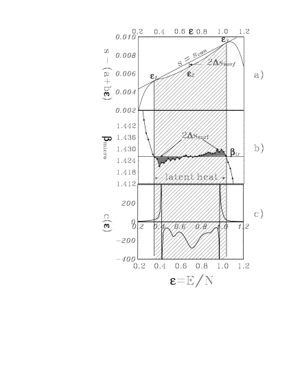
FIG. 1.: Microcanonical phase transition of first order in the Potts model, $L=200$, $q=10$.

In the CE configurations with different energies contribute $\propto exp[-N*f(\varepsilon)/T]$ to the canonical partition sum with $f(\varepsilon)=\varepsilon-Ts(\varepsilon)$ the free energy per particle. Due to the convex intruder in $s(\varepsilon)$ by $\Delta s_{surf}$ configurations with coexistent phases and energies $\varepsilon\sim\varepsilon_{2}$ are suppressed in the CE by the exponential factor $exp(-N\Delta s_{surf})=exp(-\sigma_{surf}L/T)$. This fact is frequently used in canonical model simulations of phase transitions to obtain the surface tension e.g. [11, 12].

In Fig.2 the microcanonical surface tension is shown as function of $1/L$. The surface tension deviates for a lattice of $L=12$ by only $10\%$ from the bulk values. Other parameters deviate even less from the bulk value, e.g. the transition temperature by less than $2\%$. Within the ME a phase transition can be identified with all its salient parameters, the transition temperature, the specific latent heat, the interphase surface tension, and the change of entropy per particle. It can unambiguously be identified and classified for finite systems from its microcanonical caloric equation of state $T(E/N)$. There is no need to refer to the thermodynamic limit. Evidently, the usual signal for a phase transition as a singularity in a canonical observable as function of the temperature is artificial and applies to the canonical ensemble only, c.f. e.g.[13, 4, 3]. This conclusion has far reaching consequences: One can easily extend the concept of a phase transition to systems which do not have any thermodynamic limit like e.g. selfgraviting systems or charged systems under unscreened Coulomb repulsion like hot nuclei [2].

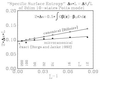
FIG. 2.: Surface tension as function of $1/L$. [9, 14, 15]

In order to test the relation of the area under the backbend of $\beta(\varepsilon)$ to the empirical bulk surface tension for a realistic system, we simulated the phase transition for evaporation and multifragmentation of some hundreds Na, K, and Fe atoms under normal pressure by our microcanonical Metropolis Monte Carlo sampling MMMC. The phase transition shows up as a clear anomaly (backbend) of the microcanonical caloric curve $T(\varepsilon)$ c.f. fig.3. It is easy to determine the transition temperature $T_{tr}$, the latent specific heat $q_{lat}$ and the surface entropy per particle $\Delta s_{surf}$. The transition is clearly identified to be of first order. In order to calculate the surface tension one has to determine the total surface area of all fragments. This is somewhat difficult as the size of the fragments drops strongly with rising excitation energy because of an increasing evaporation of monomers. In the fragmentation of Na, K clusters the total surface area keeps nevertheless roughly constant and close to $N_{0}^{2/3}$ in the first part of the transition in $\varepsilon_{1}\leq\varepsilon\leq\varepsilon_{2}$. Here the reducing size $m_{i}$ of the fragments is compensated by an increasing number of fragments $N_{fr}=\sum N_{mi\geq 2}$. Therefore, the surface tension may be estimated by formula (5), where the average is taken over the energy interval $\varepsilon_{1}\leq\varepsilon\leq\varepsilon_{2}$. As iron decays by pure monomer evaporation because of its much larger surface tension, there is only one evaporation residue with a steadily diminishing surface area and the use of formula (5) to determine the surface tension is problematic. The values of the so determined surface tension approach systematically the bulk values, table I.

$$\sigma_{surf} \sim T_{tr}*\Delta s_{surf}*N_{0}/N_{eff}^{2/3}$$ (4)

$$N_{eff}^{2/3} = <\!\!\sum_{m_{i}\geq 2}({m_{i}^{2/3}*N_{i})\!\!>},$$ (5)

FIG. 3.: Caloric curve (thick), number $N_{fr}$ of fragments with $m_{i}\geq 2$, and “number” of surface atoms $\sum(m_{i}^{2/3}N_{i})$ of microcanonical systems with 200 and 1000 sodium atoms at normal pressure.

Conclusion: Whether an interacting many-body system has a phase transition is not a property of an infinitely large system in the thermodynamic limit. One can see and classify phase transitions in finite systems by the form of the microcanonical caloric equation of state $T(E/N)$. This opens the possibility to define and discuss phase transitions also in systems which are not “thermodynamically stable” in the sense of van Hove [16]. MMMC [17, 4] allows to calculate $T(E/N)$ for some $100$ to $1000$ particles. For our examples the transition represents quite well the properties of the bulk. Configurations with coexistent, separated phases are well represented in theME whereas in the CE they are suppressed by a factor $exp(-N^{2/3}\sigma_{surf}/T_{tr})$.

	$N_{0}$	$200$	$1000$	$3000$	bulk
	$T_{tr}\;[K]$	$816$	$866$		$1156$
	$q_{lat}\;[eV]$	$0.791$	$0.871$		$0.923$
Na	$s_{boil}$	$11.25$	$11.67$		$9.267$
	$\Delta s_{surf}$	$0.55$	$0.56$
	$N_{eff}^{2/3}$	$39.94$	$98.53$		$\infty$
	$\sigma/T_{tr}$	$2.75$	$5.68$		$6.34$
	$T_{tr}\;[K]$	$697$	$767$		$1033$
	$q_{lat}\;[eV]$	$0.62$	$0.7$		$0.80$
K	$s_{boil}$	$10.35$	$10.59$		$8.99$
	$\Delta s_{surf}$	$0.65$	$0.65$
	$N_{eff}^{2/3}$	$32.52$	$92.01$		$\infty$
	$\sigma/T_{tr}$	$3.99$	$7.06$		$7.40$
	$T_{tr}\;[K]$	$2600$	$2910$	$2971$	$3158$
	$q_{lat}\;[eV]$	$2.77$	$3.18$	$3.34$	$3.55$
Fe	$s_{boil}$	$12.38$	$12.68$	$13.1$	$13.04$
	$\Delta s_{surf}$	$0.75$	$0.58$	$0.77$
	$N_{eff}^{2/3}$	$28.34$	$61.41$	$156.94$	$\infty$
	$\sigma/T_{tr}$	$5.29$	$9.44$	14.72	$16.57$

TABLE I.: Parameters of the liquid – gas transition at $1$ atm. in a microcanonical system of $N_{0}$ interacting atoms and in the bulk. The bulk values of $\sigma$ are calculated by $\sigma=4\pi r_{WS}^{2}(a_{s}-b_{s}T_{tr})$ with $a_{s}$ consistent to the value used in this calculation for the binding energies of the cluster. It was determined by [18] from experimental binding energies of different clusters. It is larger than the bulk values of [19]. As $b_{s}$ for clusters is not known and not used in this calculation it was taken from [19]. For multifragmenting Na and K the calculations are considerably more time consuming prohibiting the calculation for $N_{0}=3000$.

REFERENCES

- [1] D.H.E. Gross and R. Heck. Phys. Lett.B, 318:405–409, 1993.
- [2] D.H.E. Gross. Rep.Progr.Phys., 53:605–658, 1990.
- [3] D.H.E. Gross. In S.Albergio, S.Costa, A.Insolia, and C.Tuve, editors, Proceedings of CRIS96 ”Critical Phenomena and Collective Observables”, pages http://xxx.lanl.gov/nucl–th/9607038, Acicastello, Sicily, Italia, 27.5.-31.5.96, 1996. World Scientific, Singapore.
- [4] D.H.E. Gross. Physics Reports, in preparation, 1996.
- [5] H.O. Georgii. Journ.Stat.Phys, 80:1341–1375, 1995.
- [6] R.B. Potts. Proc.Cambridge Philos. Soc., 48:106, 1952.
- [7] K. Binder. In C. Domb and M.S. Green, editors, Phase Transitions and Critical Phenomena, New York, 1976. Academic Press.
- [8] R.J. Baxter. J. Phys., C6:L445, 1973.
- [9] D.H.E. Gross, A. Ecker, and X.Z. Zhang. Ann. Physik, 5:446–452, 1996.
- [10] D.H.E. Gross, M.E. Madjet, and O. Schapiro. HMI-preprint, http://xxx.lanl.gov/cond-mat/9608103, 1996.
- [11] K. Binder. Phys. Rev. A, 25:1699–1709, 1982.
- [12] W. Janke. Int.Journ.Mod.Phys., C 5:75, 1994.
- [13] A. Hüller. Z.Phys.B, 95:63–66, 1994.
- [14] C. Borgs and W. Janke. J. Phys. I, France, 2:2011–2018, 1992.
- [15] A. Billoire, Th. Neuhaus, and B.A. Berg. preprint Saclay, SPhT-93/065, 1993.
- [16] L. van Hove. Physica, 15:951, 1949.
- [17] D.H.E. Gross and P.A. Hervieux. Z. Phys. D, 35:27–42, 1995.
- [18] C. Bréchignac, Ph. Cahuzac, F. Carlier, M. de Frutos, J. Leygnier, J.Ph Roux, and A. Sarfati. Comments At.Mol.Phys., 31:361–393, 1995.
- [19] A. Miedema. Z.Metallkde, 69:287, 1978.