Glass phase of two-dimensional triangular elastic lattices with disorder

Abstract

We study two dimensional triangular elastic lattices in a background of point disorder, excluding dislocations (tethered network). Using both (replica symmetric) static and (equilibrium) dynamic renormalization group for the corresponding $N=2$ component model, we find a transition to a glass phase for $T<T_{g}$, described by a plane of perturbative fixed points. The growth of displacements is found to be asymptotically isotropic with $u_{T}^{2}\sim u_{L}^{2}\sim A_{1}\ln^{2}r$, with universal subdominant anisotropy $u_{T}^{2}-u_{L}^{2}\sim A_{2}\ln r$. where $A_{1}$ and $A_{2}$ depend continuously on temperature and the Poisson ratio $\sigma$. We also obtain the continuously varying dynamical exponent $z$. For the Cardy-Ostlund $N=1$ model, a particular case of the above model, we point out a discrepancy in the value of $A_{1}$ with other published results in the litterature. We find that our result reconciles the order of magnitude of the RG predictions with the most recent numerical simulations.

I Introduction

There is a lot of current interest in the problem of elastic lattices in the presence of substrate disorder. This is important in various physical systems such as flux lattices in superconductors [1], charge density waves [2], colloids and magnetic bubbles [3], Wigner crystals [4], interface roughening with disorder and solid friction of surfaces [5]. An important distinction is whether topological defects such as dislocations are present in the system or not. These defects may appear spontaneously because of disorder or not, or may be explictly excluded from the model (e.g flux lines in d=1+1 geometry [6, 7, 8], tethered networks with permanent bonds). Systems which are both elastic and periodic and do not contain topological defects are believed to form glass states with many metastable states, diverging barriers and slow dynamics [9, 10, 11, 12, 13]. There are very few analytical methods to study these states and their physics is far from being completely elucidated, despite help from extensive numerical simulations. When topological defects are present the problem is even more difficult and very little is known. A crucial question of course is whether these topological defects, when allowed in the model, will appear spontaneously at low temperature because of disorder.

The general problem of a lattice on a disordered substrate was addressed in a previous work [11, 12] and it was predicted that in $d=3$ and for weak pointlike (uncorrelated) disorder a thermodynamic phase free of unbound dislocations should exist and be stable. In this phase, called the Bragg glass, translational order decays very slowly beyond a translational quasi-order length $R_{a}$ (at most algebraically). These results [11, 12] being obtained by mapping the lattice problem onto a multicomponent version of a random field XY model the very same predictions (i.e absence of vortices and quasi long range order) obviously hold for the usual random field XY model as well. These results are at variance from previous studies which either argued for [14] or assumed [15] the spontaneous generation of dislocations, or did not address the issue [1, 16, 17, 10]. Predicted consequences [12] for the phase diagram of type II superconductors, i.e existence of a low temperature low field Bragg glass phase of vortices undergoing a transition into an amorphous state upon raising the field seem to be in agreement [18] with the most recent experiments. The existence of a $d=3$ defect free, Bragg glass type phase was confirmed in several numerical simulations either in the context of superconductors [19] or for the random field XY model [20]. Though a rigorous proof is still lacking there is also at present further theoretical support for the stability of the Bragg glass: analytical variational [7, 8] and RG studies [7] in a layered geometry and, very recently, a proof using improved scaling and energy arguments [21].

The Bragg glass is thus an example of an elastic glass phase with internal periodicity. In the physics of this type of glasses two dimensions play a particular role. In addition, further analytical methods become available [22, 23, 24] in $d=2$. When dislocations are excluded by hand, it is believed that the lower critical dimension of these elastic glasses with internal periodicity is $d_{lc}=2$, with a glass phase existing for $T<T_{g}$ in $d=2$. For the $N=1$ component model (random field XY model) this is the result of the Cardy Ostlund (CO) RG calculation [22]. By analogy it can be argued [12] that the same holds in the case of the triangular lattice, but it has not yet been directly verified. A triangular lattice requires a fully coupled $N=2$ component model. The CO $N=1$ calculation could in principle describe a $N=2$ decoupled square lattice, except that such a lattice has usually a more complicated elasticity tensor which again couples the components. When topological defects are allowed, it was shown in [22] that for the $N=1$ component model they are perturbatively relevant near the glass transition $T_{g}$. As argued in [12] $T_{g}$ for the triangular lattice is well above the KTNHY melting temperature $T_{m}$ and dislocations should then be relevant near $T_{g}$ for the $N=2$ triangular lattice as well. At low temperature however, much less is known about the importance of dislocations. The common belief [1], which is by no means rigorously established, is that if dislocations are allowed, no glass phase will exist in $d=2$. This is also hinted at by the results obtained in [25] on the simpler case of the random phase shift model, relevant to describe a lattice with internal (i.e structural) disorder [26] (a subset of the present problem). In these early studies [25, 26] the high temperature phase with unbound dislocations was found to be rentrant at low temperatures suggesting the importance of topological defects at low temperature. However, it was pointed out in [12], from a careful study of the CO RG flow, that at low temperature the scale at which the lattice is effectively dislocation-free (i.e the distance between unpaired dislocations) can be much larger than the translational length $R_{a}$. Thus even in $d=2$ the Bragg glass fixed point may be useful to describe the physics, as a very long crossover or maybe directly at $T=0$. Furthermore, it was also pointed out in [27] that the conventional CO RG will not be adequate at low temperature since it assumes a thermalized description of the vortices and neglects important effect such as the pinning of dislocations by disorder (i.e that the fugacity depends on the position). A similar idea was recently proposed by Nattermann et al. [28] who reconsidered the simpler random phase shift model. They explicitly showed that [25, 26] was incorrect at low temperature and proposed a modified coulomb gas RG. It is still an open question how these new set of ideas and techniques apply to the present problem.

In the present paper we study the statics and the dynamics of two dimensional isotropic lattices interacting with point like disorder excluding dislocations. We use a (replica symmetric) Renormalisation Group (RG) approach as well as equilibrium dynamics RG. Though we will not attempt to include dislocations, it is still interesting for several reasons. First, it is the natural continuation to $d=2$ of the non trivial fixed point which describes the Bragg glass phase for $d=3$. The only other analytical approaches available to describe the Bragg glass phase are the replica variational method [11, 29, 12] and Fisher’s functional RG [30] in a $d=4-\epsilon$ expansion [11, 12]. Thus, the study of the present fixed point in $d=2$ is also useful by comparison. Second, it is of general interest for systematic study of the $d=2$ glass phases and allows to show that the lower critical dimension is $d=2$. It is also a first step towards the study of the more difficult problem of lattices with disorder in $d=2$ with dislocations allowed. Also, since it has more parameters that the $N=1$ component model and can be similarly studied numerically, it may lead to further useful numerical checks of the replica symmetric RG in this problem as well as the dynamics (see discussion below). Finally, it may be possible to realize such tethered networks experimentally. It was argued recently [5] that internal disorder which breaks the internal periodicity of the network (and may occur in e.g polymerization) drive the system to another universality class. Even if this claim, which we will not investigate here, is correct, crossover lengths will probably be large for weak internal disorder.

The $N=1$ Cardy-Ostlund model, which is a subcase of our present calculation, has also generated a lot of attention recently, for different reasons. The gaussian replica variational method (GVM) applied to this model, leads to a one step replica symmetry breaking (RSB) solution below $T_{g}$ and to mean squared displacements which grow as $u^{2}\sim T_{g}\ln r$, a different result from the replica symmetric (RS) RG prediction $u^{2}\sim A_{1}\ln^{2}r$. Note that the GVM, being by construction an approximation which neglect some non linearities has no reason to yield the exact result (see however [31]). However it was also shown [32, 33] that the Cardy Ostlund RS-RG flow is unstable to an infinitesimal RSB perturbation at and below $T_{g}$. The issue was thus raised [32] of whether the RS-RG may miss some of the physics related to RSB. It is thus important to perform numerical simulations and carefully check the predictions of the RS-RG, as well as carefully define the observables to be computed. The numerical studies on the random phase sine-gordon model presently available show discrepancies, and their analysis is not satisfactory. In [34] no effect of disorder was found, while in [35] the results seem close to the predictions of the GVM. In the more recent [36, 37] the results seem to agree qualitatively with the RS-RG but with an amplitude much smaller than the the prediction for $A_{1}$ quoted in [38, 39] to which it was compared. Let us also point out the two very recent studies [40, 41] of the random substrate SOS model (believed to be in the same universality class) directly at zero temperature which also yield $u^{2}\sim A_{1}\ln^{2}r$.

In view of the above interest, it is thus important to compute accurately the amplitude $A_{1}$ predicted by the RS-RG. This is one of the result of the present paper. Our result, smaller by a factor of $4$ from the previous result [38, 39] is different from any of the previously published results [38, 39, 23] and, we argue, is correct. This seems to reconcile, at least in order of magnitude, the result of the RS-RG with the result of the numerical simulations of [36, 37]. A finer and more precise analysis than the one performed in [36, 37] is however needed, including predicted finite size scaling corrections, since a more careful treatment of the effects of RSB may reveal that deviations from the RS-RG result are small [42] e.g only in the amplitude of the $\log^{2}r$ [43]. Another consequence of our results is that the distribution of rescaled displacements $u/\ln r$ should be gaussian at large scale, which we propose as a useful numerical check of the RS-RG method.

Along these lines, one notes that the equilibrium dynamical RG studied here, because it obeys by construction the Fluctuation Dissipation Theorem (FDT), gives, as we illustrate explicitly, identical answers for static quantities than the replica symmetric static RG. (it thus provides for us a useful check on our statics calculations). As discussed above, it is possible that the static RG does need a RSB structure (either strong, i.e in the ground state as in mean field - or weak, i.e only in the low lying excitations) and a proposal for its construction was made in [32]. Also, we interpret the recent results [28] on the simpler random phase shift model, i.e its mapping on some version of Derrida’s random energy model, as another hint that RSB may be important in these models. If this is the case, it is then obvious that an equivalent statement should exist in the dynamics, i.e that one may need to construct a RG which violates FDT and replaces it with a generalized FDT structure, a program which was successfully carried in mean field dynamics [44, 45] We will not address this question further here but will lucidly concentrate on the predictions of the replica symmetric RG which is certainly a good starting point in this problem.

The paper is organized as follows. In Section (II) we define the model for a triangular lattice on a disordered substrate. In Section (III) we study the statics of the problem. First we use a mapping onto the replicated Coulomb gas and derive the RG equations (Section (III A). Then we analyze the RG flow and compute the correlation functions (III B). The results for the triangular lattice can be found in (III B 1). In (III B 2) we give the results for the $N=1$ Cardy Ostlund model and review the discrepancy with other published results. In Section (IV) we study the dynamics. In (IV A) we carry first order perturbation theory and in (IV B) we obtain the results for the dynamical RG. We then compute the dynamical exponent, and obtain the scaling behaviour of transport quantities at the transition. In particular we identify an “effective critical force” at the transition. Section (V) gives the conclusion. Technicalities are releguated in the appendices. In Appendix (A) we discuss in detail the regularization, obtain the RG equations and show explicitely the cutoff independence of some universal ratios. In Appendix (B) we perform the RG directly on the static replica effective action. In Appendix (III) we perform the dynamical RG to second order. In Appendix (IV) we study some consequences of the statistical tilt symmetry.

II The model

We consider a set of identical “atoms”. The interactions between them is such that the ground state configuration in the absence of disorder is a perfect triangular lattice (see fig. 1) of equilibrium positions $R_{i}^{0}$ and lattice spacing $a_{0}$. Both thermal fluctuations and disorder will result in displacements of the atoms from their ideal positions $R_{i}^{0}$ to new positions $R_{i}=R_{i}^{0}+u(R_{i}^{0})$. Furthermore the connectivity of the lattice is fixed: each site will have exactly six neighbors (see fig 1). This can be realized in principle by considering a network of identical and permanent nearest neighbor bonds (tethers) with the topology of a perfect triangular lattice. Dislocations are thus excluded in this model by construction. As discussed in the Introduction, the model can also be relevant at length scales and in regions of the phase diagram where dislocations can be neglected.

FIG. 1.: Representation of the elastic lattice and its reciprocal lattice vectors of minimal modulus.

The interaction energy can be described in terms of the local displacement field $\vec{u}(\vec{r})$ by the harmonic hamiltonian

$$H_{0}={1\over 2}\int{d^{2}\vec{q}\over(2\pi)^{2}}u_{i}(\vec{q})\Phi_{ij}(\vec{q})u_{j}(-\vec{q})$$ (1)

where $\Phi_{ij}(\vec{q})$ is the elastic matrix of the 2D lattice. In this paper we will consider isotropic (i.e triangular) lattices which can be described by only two independant elastic coefficients :

$$\Phi_{ij}(\vec{q})=c_{11}q^{2}P_{ij}^{L}+c_{66}q^{2}P_{ij}^{T}$$ (2)

where $P_{ij}^{L}=\hat{q}_{i}\hat{q}_{j}=q_{i}q_{j}/q^{2}$ and $P_{ij}^{T}=\delta_{ij}-\hat{q}_{i}\hat{q}_{j}=(\hat{q}_{\perp})_{i}(\hat{q}_{\perp})_{j}$ are respectively the longitudinal and transverse projectors.

The interaction of the lattice with the impurity disorder of the substrate is modelled by adding to the hamiltonian:

$$H_{V}=\int d^{2}\vec{x}~{}\rho(\vec{x})V(\vec{x})$$ (3)

where $\rho(\vec{x})$ is the local density of atoms, $\rho(\vec{x})=\sum_{i}\delta^{(2)}(\vec{x}-\vec{R}_{i})$. The random potential is gaussian with short range correlator $\overline{V(x)V(x^{\prime})}=h(x-x^{\prime})$. The symbol $\overline{..}$ denotes average over disorder, while $\langle..\rangle$ denotes thermal averages.

This model can be transformed, as described in details in [12] (see Section II-B), into the following random phase model:

$$\overline{Z} = \int d[u]exp~{}-{1\over T}\left(H_{0}+H_{dis}\right)$$ (4)

$${1\over T}H_{dis} = \int_{\vec{x}}\frac{1}{2}\sigma_{ij}(x)(\partial_{i}u_{j}+\partial_{j}u_{i})$$ (6)

$$+2\sqrt{g}\sum_{\nu}\cos\left(\vec{K}_{\nu}.\vec{u}(x)+\phi_{\nu}(x)\right)$$

The first terms corresponds to random local stresses and comes from the $q\sim 0$ part of the disorder[12]. The effect of only this term was studied in [26] (in the presence of dislocations), and would also arise in a problem of structural disorder (with no substrate). The second term originates from the Fourier components of the substrate potential $V_{K}$ close to one of the reciprocal lattice vectors [12]. The random field is a phase distributed uniformly over $[0,2\pi]$ and satisfies:

$$\overline{\langle e^{i(\phi_{\nu}(x)-\phi_{\nu^{\prime}}(x^{\prime})}\rangle}=\delta_{\nu,\nu^{\prime}}\delta^{(2)}(x-x^{\prime})$$ (7)

Note that we are keeping only the terms which are relevant in the RG sense near $T_{g}$. There are additional higher harmonics terms which are irrelevant in $d=2$ near $T_{g}$. There are also higher non linear terms which are small in the elastic limit $|\vec{u}(\vec{R}_{i+1})-\vec{u}(\vec{R}_{i})|\ll a$ where the derivation of (1) is valid and also irrelevant by power counting. These term will correct the bare values of the relevant coupling constants [46]

The random stress field has the general correlator:

$$\overline{\sigma_{ij}(x)\sigma_{kl}(x^{\prime})} = \frac{1}{T}[(\Delta_{11}-2\Delta_{66})\delta_{ij}\delta_{kl}$$ (9)

$$+\Delta_{66}(\delta_{ik}\delta_{jl}+\delta_{il}\delta_{jk})]$$

The bare value is $\Delta_{66}=0$ and $\Delta_{11}=\rho_{0}^{2}h_{k=0}/T$ (from [12] ) but they will flow under renormalization.

We will study both the statics and the dynamics of this model. The statics of this model can be studied using replicas to average over the disorder potential $V(\vec{x})$ [47]. The replicated model reads:

$$\overline{Z^{n}} = \int d[u^{a}]exp~{}-{1\over T}\left(H_{0}^{(n)}+H_{I}\right)$$ (10)

$$H_{0}^{(n)} = \frac{1}{2}\sum_{ab}\int_{q}[(c_{11}P_{ij}^{L}+c_{66}P_{ij}^{T})\delta_{ab}$$ (12)

$$-(\Delta_{11}P_{ij}^{L}+\Delta_{66}P_{ij}^{T})]q^{2}u^{a}_{i}(q)u^{b}_{j}(-q)$$

$$\frac{H_{I}}{T} = -g\sum_{\nu=1,2,3}\sum_{a,b=1}^{n}\cos\vec{K}_{\nu}.\left[\vec{u}^{a}(\vec{x})-\vec{u}^{b}(\vec{x})\right]$$ (13)

$g$ is related to the fourier coefficient $\Delta_{K_{0}}$ and the constant density $\rho_{0}$ : $g=\rho_{0}^{2}h_{K_{0}}/T^{2}$. We will also use the dimensionless coupling constant $\tilde{g}=ga^{2}$.

III Study of the Statics using a Coulomb gas formulation

In this Section we study the statics of the model. We first derive the renormalization group equations from a Coulomb gas formulation. In the second part we compute the static displacement correlation functions.

A derivation of the RG equations from the Coulomb gas

The model (10) is the analogue for a two-component field of the two dimensional random field XY model whose RG equations have been derived using the Coulomb Gas approach by Cardy and Ostlund[22]. But contrarily to them, our Coulomb gas formulation[48, 49, 50] is obtained by first using a Villain approximation[51] before averaging over the disorder. This results in a natural coupling between the continuous replicated displacement field $u^{a}(\vec{x})$ and vector charges $\vec{n}^{a}_{\nu}(\vec{x})=n^{a}(\vec{x},\nu).\vec{K}_{\nu}$ where $\vec{K}_{\nu}$ is one of the three ($\nu=1,2,3$) reciprocal lattice vector of minimal modulus (see fig 1) and $n^{a}(\vec{x},\nu)\in{\mathbb{Z}}^{n}$ :

$$\overline{{Z}^{n}}=\int d[u^{a}]\ \sum_{[n_{\nu}^{a}(\vec{x})]}\ \exp\ \Biggl{(} -{1\over T}H_{0}^{n}-i\ \int_{\vec{r}}\vec{n}_{\nu}^{a}.\vec{u}^{a}(\vec{r})$$ (15)

$$+\int_{\vec{r}}\ln(\sqrt{g})\sum_{a,\nu}\left(\vec{n}^{a}\right)^{2}(\vec{r},\nu)\Biggr{)}$$

with the condition $\forall(\vec{x},\nu)\ \ \sum_{a}n^{a}(\vec{x},\nu)=0$. The RG equations will be derived to lowest order in the charge fugacity $\sqrt{g}$, since higher order operators are irrelevant near the critical point[52] : thus we can only consider charges of the form $n^{a}(x,\nu)=\delta_{\alpha}^{a}-\delta_{\beta}^{a}\equiv\delta_{\alpha,\beta}^{a}$ where $\alpha$ and $\beta$ are replica integers between $0$ and $n$. The effective fugacity of these minimal charges is $g$. Integrating over the smooth field $u(\vec{x})$ one recover a 2D vector Coulomb Gas with charges having both a spatial and a replica structure, and whose action is (omitting the fugacity term):

$$S[n] = {T\over 2}\sum_{\nu,\nu^{\prime}}\int_{\vec{q}}\vec{n}^{a}_{\nu,i}(q)(\Phi^{-1})_{ij}^{ab}\vec{n}^{b}_{\nu^{\prime},j}(-q)$$ (16)

$$= -{T\over 2}\sum_{\nu,\nu^{\prime}}\int_{\vec{r},\vec{r}^{\prime}}\vec{n}_{\nu,i}^{a}(\vec{r})V_{ij}^{ab}(\vec{r}-\vec{r}^{\prime})\vec{n}_{\nu,j}^{b}(\vec{r}^{\prime})$$ (17)

where the interaction $V(\vec{r})$ is obtained by a Fourier transform. We have incorporated the replica off diagonal terms in $\Phi^{-1}_{ab}$.

In this section, as is usualy done, we will use[53], instead of the full interaction, its asymptotic form[49] ($r\gg a$) (see Appendix A) :

$$V_{ij}(\vec{r})=\delta_{ij}\left({\kappa}^{ab}_{1}\ln{r\over a}+\frac{1}{2}{\kappa}^{ab}_{2}\right)\ \ -{\kappa}^{ab}_{2}\ {r_{i}r_{j}\over r^{2}}$$ (18)

and ${\kappa}^{ab}_{1}=\left(c_{66}^{-1}+c_{11}^{-1}\right)^{ab}/4\pi$, ${\kappa}^{ab}_{2}=\left(c_{66}^{-1}-c_{11}^{-1}\right)^{ab}/4\pi$. We will use the notation ${\kappa}^{ab}_{1}={\kappa}_{1}\delta_{ab}-\overline{{\kappa}_{1}}$ and $\left(c_{11}\right)^{ab}=c_{11}\delta^{ab}-\Delta_{11}$.

We won’t deal with possible appearence of dislocations in this model. This will lead to an electromagnetic vector CG which neads more work[54]. This simplification allows us to derive RG equations by working on the 2-point correlation function[55] instead of the replicated partition function[50, 49]. These two schemes are equivalent[56] to order (at least) $g^{2}$. The renormalised elastic matrix can be defined as

$$q^{2}\left(\Phi_{R}^{-1}\right)_{ij}^{ab} = (c_{11,R}^{-1})^{ab}P_{ij}^{L}+(c_{66,R}^{-1})^{ab}P_{ij}^{T}$$ (19)

$$= \lim_{q\rightarrow 0}{q^{2}\over T}\langle u_{i}^{a}(\vec{q})u_{j}^{b}(-\vec{q})\rangle$$ (20)

To be consistent this definition must be independant of the direction $\hat{q}$ : this is simply a direct consequence of the isotropic nature of the 2nd order invariant tensors on the triangular lattice. The explicit expression for the renormalised elastic coefficients naturally follows :

$$\left(c_{11,R}^{-1}-c_{11}^{-1}\right)^{ab}=$$ (21)

$$-T\lim_{q\rightarrow 0}q^{2}\langle\vec{n}^{c}_{\nu,l}(\vec{q})\vec{n}^{d}_{\nu^{\prime},m}(-\vec{q})\rangle_{S[n]}P_{ij}^{L}\left(\Phi^{-1}\right)_{il}^{ac}\left(\Phi^{-1}\right)_{jm}^{bd}$$ (22)

where $i,j,l,m$ are cartesian coordinates, and we used the notation $\vec{n}^{c}_{\nu,l}=n^{c}\times\left(\vec{K}_{\nu}\right)_{l}$. The same holds for $c_{66}^{-1}$ by simply replacing $P_{ij}^{L}$ by $P_{ij}^{T}$.

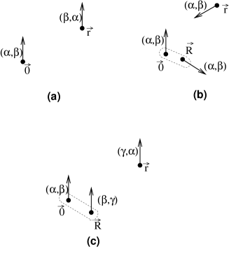
FIG. 2.: Representation of the three different configurations that contribute to the correlation function of the Coulomb Gas charge $\vec{n}$. Configuration (a) is of order $g^{2}$ whereas (b) and (c) are of order $g^{3}$.

Replacing $\Phi^{-1}$ by its expression (2) and using the Fourier transform of the charge correlation, we obtain

$$\left(c_{11,R}^{-1}\right)^{ab}=\left(c_{11}^{-1}\right)^{ab} + {T\over 2}P_{ij}^{L}\left(c_{11}^{-1}\right)^{ac}\left(c_{11}^{-1}\right)^{bd}$$ (23)

$$\times \int_{\vec{r}}(\hat{q}.\vec{r})^{2}\langle\vec{n}_{\nu,i}^{c}(\vec{0})\vec{n}_{\nu^{\prime},j}^{d}(\vec{r})\rangle_{S[n]}$$ (24)

This equation is the starting point of our RG study. Note that itis a definition of the renormalised elastic coefficient exact to all order in $g$. We now proceed as follow : first we expand perturbatively in $g$ the right-hand side of this equation. One can then apply a coarse-graining procedure which leaves the form of this perturbative expansion unchanged, thus defining coarse-grained elastic coefficients. To order $g^{3}$ only three terms appear (see fig.2) : (a) of order $g^{2}$ and (b) and (c). Corrections coming from the coarse-graining of configuration (a) defines the coarse-grained elastic constant $c_{11}^{-1}(l)$ to order $g^{2}$ and $g(l)$ to order $g$, where $l$ is the scaling parameter. In the spirit of Coulomb Gas renormalisation[48], this corresponds to the annihilation of charges (screening of the coulomb interaction), whereas the fusion of charges is given by the contributions of configurations (b) and (c) when $|\vec{R}|\ll|\vec{r}|$ or when $|\vec{R}-\vec{r}|\ll|\vec{r}|$. This gives the correction of $g(l)$ to order $g^{2}$.

First, let us develop the two point correlation function $\langle\vec{n}_{\nu,i}^{c}(\vec{0})\vec{n}_{\nu^{\prime},j}^{d}(\vec{r})\rangle$ to order $g^{3}$ : it is given by the three contributions (a), (b), and (c) (see fig 2) :

$$\langle\vec{n}_{\nu,l}^{c}(\vec{0})\vec{n}_{\nu^{\prime},m}^{d}(\vec{r})\rangle_{S[n]}=g^{2}{\cal A}_{1}(\vec{0},\vec{r})+g^{3}{\cal A}_{2}(\vec{0},\vec{r})$$ (25)

where the first term corresponds to the only neutral 2-charges configuration :

$${\cal A}_{1}(\vec{0},\vec{r})=\sum_{\nu}\sum_{\alpha\neq\beta}^{n}\delta^{c}_{\alpha,\beta}\delta^{d}_{\beta,\alpha}(K_{\nu})_{l}(K_{\nu})_{m}e^{-S_{a}}$$ (26)

and configurations (b) and (c) contribute to the factor ${\cal A}_{2}$ :

$${\cal A}_{2}(\vec{0},\vec{r}) = 2\int_{\vec{R}}\sum_{\nu\neq\nu^{\prime}}\sum_{\alpha\neq\beta}^{n}\delta^{c}_{\alpha,\beta}\delta^{d}_{\alpha,\beta}(K_{\nu})_{l}(K_{\nu^{\prime}})_{m}e^{-S_{b}}$$

$$+ 2\int_{\vec{R}}\sum_{\nu}\sum_{\alpha\neq\beta\neq\gamma}^{n}\delta^{c}_{\alpha,\beta}(\delta^{d}_{\beta,\gamma}+\delta^{d}_{\gamma,\alpha})(K_{\nu})_{l}(K_{\nu})_{m}e^{-S_{c}}$$

In these expressions, $S_{a},S_{b},S_{c}$ are the respective actions of the three configurations : $S_{a}=2T|\vec{K}|^{2}\left({\kappa}_{1}\ln(r/a)-{\kappa}_{2}(\hat{K}.\hat{r})^{2}+\kappa_{2}/2\right)$. The two others can be easily expressed in terms of $S_{a}$. We can put this back in the expression (23) of $c_{11,R}^{-1}$. The angular integral of the $g^{2}$ term can be performed, using the parameter $\alpha={\kappa}_{2}|\vec{K}|^{2}T$ :

$$B_{\stackrel{{\scriptstyle{\scriptstyle 11}}}{{\scriptstyle 66}}}(\alpha) = \sum_{\nu}\int d\hat{r}\left(\hat{q}.\hat{r}\right)^{2}\left(\hat{q}_{\stackrel{{\scriptstyle{\scriptstyle\parallel}}}{{\scriptstyle\perp}}}.K_{\nu}\right)^{2}e^{2\alpha(\hat{K}.\hat{r})^{2}-\alpha}$$ (27)

$$= K^{2}{3\pi\over 4}\left(\pm I_{1}(\alpha)+2I_{0}(\alpha)\right)$$ (28)

where $I_{0}$ and $I_{1}$ are the modified Bessel functions. The function $B_{11}$ appears in the expression of $c_{11,R}^{-1}$ while $c_{66,R}^{-1}$ involves $B_{66}$. Using the following results on the replicated charges

$$\sum_{\alpha,\beta}\delta^{a}_{\alpha,\beta}\delta^{b}_{\beta,\alpha}=-2\left(n\delta^{ab}-1\right)$$

$$\sum_{\alpha\neq\beta\neq\gamma}\delta^{a}_{\alpha,\beta}\delta^{b}_{\beta,\gamma}=(2-n)\left(n\delta^{ab}-1\right)$$

and the definition $\tilde{g}=ga^{2}$, we can express $c_{11,R}^{-1}$ as

$$\left(c_{11,R}^{-1}\right)^{ab}=\left(c_{11}^{-1}\right)^{ab}(l)$$ (29)

$$- {T\over c_{11}^{2}}\tilde{g}^{2}(l)(n\delta^{ab}-1)B_{11}(\alpha)\int_{a}^{\infty}{dr\over a}\left({r\over a}\right)^{3-2|\vec{K}|^{2}K_{1}T}$$ (31)

$$+{T\over c_{11}^{2}}\tilde{g}^{3}(l)(n\delta^{ab}-1)\int_{|\vec{r}|\geq a}{d^{2}\vec{r}\over a^{2}}K^{2}\Lambda(\vec{r})$$

The integrand in the last term is given by :

$$\Lambda(\vec{r})=\int_{|\vec{R}|\geq a}{d^{2}\vec{R}\over a^{2}}{3\over 8} \left({r\over a}\right)^{2}\left(\cos 2(\hat{K},\hat{r})+2\right)$$

$$\times\left((2-n)e^{-S_{c}}-e^{-S_{b}}\right)$$

We can then apply the coarse-graining procedure to this self-consistent equation. We thus rescale the hard-core cut-off from $a$ to $\tilde{a}=ae^{dl}\approx a+adl$. The first integral split into two terms $(\eta=|\vec{K}|^{2}{\kappa}_{1}T)$ :

$$\int_{a}^{\infty}{dr\over a}\left({r\over a}\right)^{3-2\eta} \longrightarrow \int_{a}^{ae^{dl}}\frac{dr}{a}\left({r\over a}\right)^{3-2\eta}+\int_{ae^{dl}}^{\infty}\frac{dr}{a}\left({r\over a}\right)^{3-2\eta}$$

$$\approx dl+e^{l(4-2\eta)}\int_{\tilde{a}}^{\infty}\frac{dr}{\tilde{a}}\left({r\over\tilde{a}}\right)^{3-2\eta}$$

Hence the first terms contribute to $c_{11}^{-1}(l)$ while the second renormalises $\tilde{g}(l)$ :

$$d\ [c_{11}^{-1}]^{ab}(l) = -\tilde{g}^{2}(n\delta^{ab}-1)TB_{11}(\alpha)c_{11}^{-2}~{}dl$$ (32)

$$d\ \tilde{g}^{2}(l) = (4-2|\vec{K}|^{2}{\kappa}_{1}T)\tilde{g}^{2}~{}dl$$ (33)

For the purpose of this paper, we are only interested in the contribution of the last term of eq. (29) to $dg^{2}$. It corresponds to configuration (b) and (c) of (fig.2), when $a\leq|\vec{R}|\leq a(1+dl)$ or $a\leq|\vec{R}-\vec{r}|\leq a(1+dl)$.

The renormalisability of the model that one can directly see in our procedure ensures that this correction can be written as a a contribution to $\tilde{g}^{2}(l)$ of order $\tilde{g}^{3}$. First of all we check these renormalisation properties of the hamiltonian :

$$\lim_{|\vec{R}|\rightarrow a}e^{-S_{b}(\vec{r},\vec{R})}=e^{-S_{a}(\vec{r})}\ e^{-2\alpha(\hat{K}_{1}.\hat{R})(\hat{K}_{2}.\hat{R})-\frac{\alpha}{2}}$$

$$\lim_{|\vec{R}|\rightarrow a}e^{-S_{c}(\vec{r},\vec{R})}=e^{-S_{a}(\vec{r})}\ e^{\alpha(\hat{K}_{1}.\hat{K})^{2}-\frac{\alpha}{2}}$$

The corresponding correction is

$$\delta\Lambda(\vec{r})={3\over 4}\left({r\over a}\right)^{2}\left(\cos 2(\hat{K},\hat{r})+2\right)e^{-S_{a}}B_{g}(\alpha)$$ (34)

where the fonction $B_{g}(\alpha)$ is given by

$$B_{g}(\alpha) = \int d\hat{R}e^{-\alpha/2}[(2-n)e^{\alpha\cos^{2}(\hat{K},\hat{R})}$$ (36)

$$~{}~{}~{}~{}~{}~{}~{}~{}~{}~{}~{}~{}~{}~{}~{}-e^{-2\alpha\cos(\hat{K},\hat{R})\cos(\hat{K}^{\prime},\hat{R})}]$$

$$= 2\pi\left[(2-n)I_{0}(\alpha/2)-I_{0}(\alpha)\right]$$ (37)

Integration over $\vec{r}$ leads to

$$\int{d^{2}\vec{r}\over a^{2}}K^{2}\delta\Lambda(\vec{r})=2B_{g}(\alpha)B_{11}(\alpha)\int_{a}^{\infty}{dr\over a}\left({r\over a}\right)^{3-2K^{2}{\kappa}_{1}T}$$

This is exactly the expected form, which can be written as a correction to $g^{2}$ :

$$d(g^{2})=-dl~{}\tilde{g}^{3}2B_{g}(\alpha)$$ (38)

where

$$B_{g}(\alpha)=-2\pi\left(I_{0}(\alpha)+(n-2)I_{0}(\alpha/2)\right)$$

The final equations, obtained after the $n\rightarrow 0$ limit, are

$${d\ c_{11}\over d\ l} = {d\ c_{66}\over d\ l}=0$$ (40)

$${d\ \Delta_{11}(l)\over d\ l} = \tilde{g}^{2}TB_{11}(\alpha)$$ (41)

$${d\ \Delta_{66}(l)\over d\ l} = \tilde{g}^{2}TB_{66}(\alpha)$$ (42)

$${d\ \tilde{g}\over d\ l} = (2-K^{2}{\kappa}_{1}T)\tilde{g}-\tilde{g}^{2}B_{g}(\alpha)$$ (43)

with $\tilde{g}=ga^{2}$. From now on $B_{g}(\alpha)$ denotes its value at $n=0$.

It is useful to compare these equations with the one for the $n=1$ component model of Cardy and Ostlund. To obtain them we set $c_{11}=c_{66}=c$ (i.e $\alpha=0$), $\Delta_{11}=\Delta_{66}=\Delta$ and consider the two reciprocal lattice vectors (instead of three) of a square lattice in the interaction term with $K^{2}=1$. This gives two decoupled $n=1$ component model with RG equations obtained by $B_{11}=B_{66}\to\pi$ and drop the term not proportional to $n-2$ in the $g^{2}$ correction.

$${dc\over dl} = 0$$ (45)

$${d\Delta(l)\over dl} = \pi\tilde{g}^{2}T$$ (46)

$${d\tilde{g}\over d\ l} = (2-\frac{T}{2\pi c})\tilde{g}-4\pi\tilde{g}^{2}$$ (47)

the transition temperature is thus $T^{CO}_{g}=4\pi c$.

B Analysis of the RG flow and static correlation functions

We now study the RG flow and compute the correlations. In the case of the $N=1$ model this was first done in [22, 23] and later reconsidered in [24, 57].

1 triangular lattice

The flow defined by the above RG equations (III A) has similarities with the one obtained for the random field XY model[22]. There is a transition at $T_{g}=2/(K^{2}\kappa_{1})=8\pi K^{-2}c_{11}c_{66}/(c_{11}+c_{66})$ and one has $K^{2}=16\pi^{2}/3a_{0}^{2}$ for the triangular lattice.

In the high temperature phase $T>T_{g}$ the disorder renormalizes to zero. At low temperature $T<T_{g}$ the coupling constant $\tilde{g}(l)$ converges towards a perturbative fixed point $\tilde{g}^{*}$. Introducing the reduced temperature $\tau=(T_{g}-T)/T_{g}$, one has: $\tilde{g}^{*}=2\tau/B_{g}(\alpha)$ with $B_{g}(\alpha)=2\pi(2I_{0}(\alpha/2)-I_{0}(\alpha))$. It depends continuously on the value of $\alpha$, defined in (27) and which we can evaluate at $T_{g}$ since we work near $T_{g}$. Using the above value for $T_{g}$ one finds that $\alpha(T_{g})=\alpha_{g}=2(c_{11}-c_{66})/(c_{11}+c_{66})=2(1+\sigma)/(3-\sigma)$ where $\sigma$ is the Poisson ratio defined as usual as $\sigma=1-2c_{66}/c_{11}=\lambda/(\lambda+2\mu)$. Thus we find that the obtained fixed point depends continuously on the Poisson ratio. Since the Poisson ratio is not renormalized one has now a plane of fixed points, rather than a line in the case of the $N=1$ Cardy Ostlund model, parametrized by the temperature $\tau$ and the Poisson ratio $\sigma$.

One must check however that the perturbative fixed point does indeed exist, i.e that $B_{g}(\alpha)>0$ on the allowed domain of variations of $\alpha$. This is indeed the case since one finds that $B_{g}(\alpha)>0$ as long as $\alpha\leq\alpha^{*}\approx 2.218$. This condition is fullfilled since $c_{66}>0$ implies that $\alpha<2$.

At this fixed point both $\Delta_{11}(l)$ and $\Delta_{66}(l)$ grow to non perturbative values. This is not a problem since due to statistical symmetry [58] they do not feedback in the RG equations. This produces however a change in the correlation functions (see e.g Appendix IV).

We can integrate the above RG equations and the solution reads:

$$\tilde{g}(l) = \frac{g_{0}e^{2\tau l}}{1+\chi(e^{2\tau l}-1)}$$ (48)

$$\Delta_{11,66}(l) = \Delta(0)+\frac{D_{11,66}}{2\tau}\Biggl{(}\ln(1+\chi(e^{2\tau l}-1))$$ (50)

$$-\chi(1-\chi)\frac{e^{2\tau l}-1}{1+\chi(e^{2\tau l}-1)}\Biggr{)}$$

where we defined $D_{11,66}=4\tau^{2}TB_{11,66}(\alpha)/B_{g}^{2}(\alpha)$ and $\chi=g_{0}B_{g}(\alpha)/(2\tau)$. Note that $\chi=g_{0}/\tilde{g}^{*}$ for $\tau>0$. Thus at large $l$ one has in the glass phase ($\tau>0$):

$$\tilde{g}(l)=\tilde{g}^{*}+{\cal O}(e^{-2\tau l})$$ (51)

$$\Delta_{11,66}(l)=D_{11,66}\ln\left(\frac{ae^{l}}{\xi}\right)+\Delta_{11,66}(0)+{\cal O}(e^{-2\tau l})$$ (52)

where we have introduced the length:

$$\xi=a\exp\left(\frac{1-\chi-\ln\chi}{2\tau}\right)$$ (53)

For weak disorder $g_{0}\ll 2\tau/B_{g}$ it corresponds to the length $\xi\sim R_{a}\sim(2\tau/g_{0})^{1/(2\tau)}\gg a$ at which translational order decays asymptotically (also equal to the Larkin length $R_{c}$ for this lowest harmonic model [7], valid near $T_{g}$). Note that one can define another length scale $\xi_{c}$ defined as the crossover length between a $\log(r)$ behaviour of the mean squared displacements (see below) for $r<\xi_{c}$ to a large $r$ regime which corresponds to a $\log^{2}(r)$ asymptotic correlation. This length diverges exponentially as $\xi_{c}\sim exp(-cst/\tau^{2})$ at the transition $\tau=0$.

We now compute the correlation functions [24]. We will be interested in the following correlation functions:

$$B_{ij}(r) = \overline{\langle(u_{i}(\vec{r})-u_{i}(\vec{0}))(u_{j}(\vec{r})-u_{j}(\vec{0}))\rangle}$$ (54)

$$= 2\int{d^{2}\vec{q}\over(2\pi)^{2}}(1-e^{i\vec{q}.\vec{r}})\overline{\langle u_{i}(\vec{q})u_{j}(-\vec{q})\rangle}$$ (55)

$$= B_{L}(r)\tilde{P}_{ij}^{L}+B_{T}(r)\tilde{P}_{ij}^{T}$$ (56)

where the projectors are defined by $\tilde{P}_{ij}^{L}=\hat{r}_{i}\hat{r}_{j}$ and $\tilde{P}_{ij}^{T}=(\hat{r}_{\perp})_{i}(\hat{r}_{\perp})_{j}$. The longitudinal correlator is thus given by

$$B_{L}(r)=2\int{d^{2}\vec{q}\over(2\pi)^{2}}\left(1-e^{i\vec{q}.\vec{r}}\right)\tilde{P}_{ij}^{L}\overline{\langle u_{i}(\vec{q})u_{j}(-\vec{q})\rangle}$$ (57)

The transverse correlation function follows by replacing $\tilde{P}^{L}$ by $\tilde{P}^{T}$.

We define

$$\Gamma_{ij}(\vec{q},\Delta_{11,66}(0),\tilde{g}(0))=\overline{\langle\vec{u}_{i}(\vec{q})\vec{u}_{j}(-\vec{q})\rangle}$$ (58)

Using usual dimensional scaling relations, we can write

$$\Gamma_{ij}(\vec{q},\Delta_{11,66}(0),\tilde{g}(0))=e^{2l}~{}\Gamma_{ij}(e^{l}\vec{q},\Delta_{11,66}(l),\tilde{g}(l))$$

We then choose the scaling parameter $l$ such that[24] $qe^{l}=1/a$. The large $r$ behaviour of the correlation function thus corresponds to the limit $e^{l}\rightarrow\infty$. The RG flow approaches its fixed point in that limit : $\tilde{g}\rightarrow\tilde{g}^{\infty}\approx\tilde{g}^{*}$. Assuming that $\Gamma_{ij}(1/a,\Delta_{11,66}(l),\tilde{g}^{*})$ can be evaluated perturbatively in $\tilde{g}^{*}$ near $T_{c}$ We can then evaluate the correlation function :

$$\Gamma_{ij}(\vec{q},\Delta_{11,66}(0),\tilde{g}(0))=$$ (59)

$${T\over q^{2}}\left((c_{11}^{-1}+{\Delta_{11}(l)\over c_{11}^{2}})P^{L}_{ij}+(c_{66}^{-1}+{\Delta_{66}(l)\over c_{66}^{2}})P^{T}_{ij}\right)$$ (60)

The correlation function then takes the following form near $T_{g}$:

$$\overline{\langle\vec{u}_{i}(\vec{q})\vec{u}_{j}(-\vec{q})\rangle}\stackrel{{\scriptstyle q\rightarrow 0}}{{\simeq}} -{T_{g}\over q^{2}}\ln(q\xi)\left({D_{11}\over c_{11}^{2}}P_{ij}^{L}+{D_{66}\over c_{66}^{2}}P_{ij}^{T}\right)$$ (61)

The angular integrals can be easily performed using the formula:

$${1\over 2\pi}\int d\hat{q}(1-e^{i\vec{q}.\vec{r}})P_{ij}^{\alpha}\tilde{P}_{ij}^{\beta}={1\over 2}\left(1-J_{0}(qr)+\epsilon_{\alpha\beta}J_{2}(qr)\right)$$ (62)

with $\alpha,\beta=L,T$ and $\epsilon_{LL}=\epsilon_{TT}=1$ and $\epsilon_{LT}=\epsilon_{TL}=-1$.

This gives:

$$B_{L,T}(r) = {1\over 2\pi}(\tilde{B}_{11}+\tilde{B}_{66})\int\frac{dq}{q}\ln(1/(q\xi))(1-J_{0}(qr))$$ (64)

$$\pm{1\over 2\pi}(\tilde{B}_{11}-\tilde{B}_{66})\int\frac{dq}{q}\ln(1/(q\xi))J_{2}(qr)$$

where $\tilde{B}_{11,66}=T_{g}D_{11,66}/c_{11,66}^{2}$. The integrals can be evaluated as:

$${1\over 2\pi}\int_{0}^{{2\pi\over a}}dq{\ln(q\xi)\over q}\left(1-J_{0}(qr)\right)$$

$$=-{1\over 4\pi}\ln^{2}\left({r\over\xi}\right)+{\cal O}\left(\ln\left({r\over a}\right)\right)$$

$${1\over 2\pi}\int_{0}^{{2\pi\over a}}dq{\ln(q\xi)\over q}J_{2}(qr)$$

$$=-\frac{1}{4\pi}\left(\ln\left({r\over\xi}\right)\right)+{\cal O}\left(1\right)$$

The difference between the expressions of $B_{L}$ and $B_{T}$ is the sign of the second order Bessel function $J_{2}(qr)$. Both these correlations have the same leading term in the limit of large $r$, given to the lowest order in $\tau$ by:

$$B_{L}(r)\sim B_{T}(r)\sim\frac{b(\alpha)}{K^{2}}\tau^{2}\ln^{2}\left({r\over\xi}\right)$$ (65)

with a universal coefficient (the cut-off dependence drops out) $b(\alpha)=(\tilde{B}_{11}+\tilde{B}_{66})/(4\pi)$ Another universal quantity (in the limit of large $r$) is the difference $B_{T}(r)-B_{L}(r)$ since the leading integral, with all its cutoff dependent corrections in $\ln r/a$ cancel exactly. One obtains:

$$B_{T}(r)-B_{L}(r)\sim\frac{\tilde{b}(\alpha)}{K^{2}}\tau^{2}\ln\left({r\over\xi}\right)$$ (66)

The coefficient of the log is a universal function of $c_{11}$ and $c_{66}$, $\tilde{b}(\alpha)=(\tilde{B}_{66}-\tilde{B}_{11})/(4\pi)$. Specifically one finds (see fig.3 for a plot of these functions) :

$$b(\alpha)=6\frac{2I_{0}(\alpha)(1+\frac{\alpha^{2}}{4})-\alpha I_{1}(\alpha)}{(2I_{0}(\alpha/2)-I_{0}(\alpha))^{2}}$$ (67)

$$\tilde{b}(\alpha)=6\frac{I_{1}(\alpha)(1+\frac{\alpha^{2}}{4})-2\alpha I_{0}(\alpha)}{(2I_{0}(\alpha/2)-I_{0}(\alpha))^{2}}$$ (68)

where $\alpha=\alpha_{g}=2(c_{11}-c_{66})/(c_{11}+c_{66})$.

Here it is interesting to remark that in addition to the two terms (65,66), $B_{L,T}(r)$ contains a non universal term proportional to $\ln(r/a)$ (e.g a term like $\Delta(0)\ln(r/a)$). Therefore when comparing the RG predictions with e.g numerical results, one should be careful in identifying the different components of the spatial correlations.

FIG. 3.: Plot of the numerical coefficients of the correlation functions $B_{T,L}(r)$ and $B_{T}(r)-B_{L}(r)$ : $b(\alpha)$ and $\tilde{b}(\alpha)$ as function of the elastic ratio $\alpha=2(1+\sigma)/(3-\sigma)$. We have also plotted the coefficient of the dynamical exponent : $\theta(\alpha)=(z-2)/\tau$. $\theta_{co}$, the corresponding value for the planar random field XY model (the Cardy-Ostlund model) is shown as a reference. See the text for the details.

As we discuss in the Appendix IV the distribution of rescaled displacements $u/\ln r$ should be gaussian. Thus we have also obtained the decay of the structure factor at large $r$:

$$C_{K_{0}}(r)=\overline{e^{iK_{0}.u(r)}e^{-iK_{0}.u(0)}}\sim\exp(-\frac{1}{2}b(\alpha)\tau^{2}\ln^{2}({r\over\xi}))$$ (70)

the corresponding result for the $N=1$ CO model structure factor is given in 10 of the Appendix IV. Though the $\ln^{2}r$ term is isotropic there is subdominant anisotropy. For instance one has for the decay in different directions:

$$\frac{C_{K_{0}}(r\parallel K_{0})}{C_{K_{0}}(r\perp K_{0})}\sim(\frac{\xi}{r})^{\frac{\tilde{b}(\alpha)\tau^{2}}{2}}$$ (71)

which is the analogous for $d=2$ of Eq. (4.32) of Ref. [12].

High temperature phase

Finally, the high temperature phase is characterised by $\tilde{g}(l\rightarrow\infty)=0$ and a non universal value of $\Delta_{i}(l)\rightarrow\Delta^{\infty}_{i}$. From (48) we find

$$\Delta^{\infty}_{11,66}=\Delta_{11,66}(0)+\frac{D_{11,66}}{2\tau}\left(\ln(1-\chi)+\chi\right)$$ (72)

which depends on the initial bare values of $\Delta$ but remains finite at the transition $\tau\to 0^{-}$.

Since the renormalised theory is gaussian, the correlation function is straightforwardly given in the limit of large $r$ by:

$$\overline{\langle(u_{i}(\vec{r})-u_{i}(\vec{0}))(u_{j}(\vec{r})-u_{j}(\vec{0}))\rangle}\sim$$ (73)

$${T\over\pi}\delta_{ij}\ln\left({r\over a}\right)\left((c_{11}^{-1}+{\Delta_{11}^{\infty}\over c_{11}^{2}})+(c_{66}^{-1}+{\Delta_{66}^{\infty}\over c_{66}^{2}})\right)$$ (74)

2 Cardy-Ostlund model

In the case of the Cardy Ostlund $N=1$ problem, defined in its replicated version, as:

$$\frac{H}{T} = \sum_{ab}\int_{r}(\frac{1}{2T}(c\delta_{ab}-\Delta_{ab})\nabla u_{a}\nabla u_{b}-g\cos(K(u_{a}-u_{b}))$$ (75)

one finds, using (III A):

$$B(r)=\overline{\langle(u(r)-u(0))^{2}\rangle}\sim\frac{2}{K^{2}}\tau^{2}\ln^{2}(r/\xi)$$ (76)

where, we recall $\tau=(T_{g}-T)/T_{g}$. As announced in the Introduction, this result is different from all the results previously published (to our knowledge). Since it is important for comparison with several existing numerical simulations, we now discuss in more details this discrepancy.

Our result is smaller by a factor of $2$ from the original result (5.24) of Ref. [23]. It is smaller by a factor of $4$ from the result quoted in Ref. [38], and still by a factor of $2$ from its later corrected value [59] (it is also larger by a factor of $4$ from the result obtained in [57]).

As discussed above the RG equations which read at $T_{g}$, $d\Delta/dl=c_{1}g^{2}$, $dg/dl=c_{2}g^{2}$ are not universal but the following amplitude ratio, defined in [38] $R=T_{g}c_{1}/(cc_{2})^{2}$ is universal. We find here that $R=\pi$. (as well as in Ref. [7]). This is also the valued we inferred from the static and dynamic RG equations of [23, 60] and we thus agree with their RG equations. This value was $R=2\pi$ and thus incorrect in [38] but later corrected back to $R=\pi$ [59].

The origin of the discrepancy between (76) and the result (5.24) of Ref. [23] thus lies in the calculation of the correlation function. It can probably be traced to the algebraic mistake between equations (5.23) and (5.24) of Ref. [23]. Finally the discrepancy with [57] lies first in their RG equations with $N=1$ (we extracted their amplitude ratio as being $R=\pi/2$) and later in a factor of two in the calculation of the correlations (correcting for the additional misprint between formulae (13) and (14)).

As discussed in the Introduction this improves the comparison between numerical simulations and the RS-RG. Indeed in Ref. [36] a result smaller by a factor of $5$ than [38] was found, and we find here a result smaller than [38] by a factor of $4$. Concerning the recent quoted results [40] of the numerical determination of the ground state, we find that it is about twice the naive continuation of our amplitude to $T=0$, i.e setting ($\tau=1$) in the above result (76).

IV Dynamics

In this section we study the dynamics of the triangular lattice on a disordered substrate. We study directly the dynamics of the original random sine gordon model (6). The method we use is to perform the renormalisation on the dynamical effective action associated to (6) and compute dynamical quantities. We find that this method is more convenient, and leads to more tractable calculations, than the method [60, 61] originally used by Goldschmidt and Schaub to study the dynamics of the Cardy-Ostlund model. In order to obtain the dynamical exponent $z$ one needs, in addition to purely dynamical quantities, some information on the statics. It would be potentially erroneous to attempt to extract from the previous Section the necessary information on the statics, since we used in the previous Section a different method with a different regularisation scheme. Instead, the consistent approach is to use the same method and the same regularisation scheme in the statics and the dynamics. We will thus carefully reobtain the results for the statics within the same dynamical RG. This is possible, as we will demonstrate, because we are studying the equilibrium dynamics. Using the fluctuation dissipation theorem (FDT), which then holds exactly by assumption, one can then reobtain the statics. We will also show (see Appendix B) that the same effective action method, but applied to the replica symmetric theory gives the same results for the static as the FDT equilibrium dynamics. Also clearly demonstrate how the cutoff dependence comes in the RG equations and how at $T=T_{g}$ the physical amplitudes become universal, as detailed in Appendix A.

A perturbation theory on the dynamical action

The dynamics of the model (6) can be described by a Langevin type equation:

$$\eta\frac{\partial}{\partial t}u^{\alpha}(x,t)=-\frac{\delta H}{\delta u^{\alpha}(x,t)}+\zeta^{\alpha}(x,t)$$ (77)

with $\langle\zeta^{\alpha}(x,t)\zeta^{\beta}(x^{\prime},t^{\prime})\rangle=2\eta T\delta_{\alpha\beta}\delta(x-x^{\prime})\delta(t-t^{\prime})$ being the thermal noise and $\eta$ is the friction coefficient. The hamiltonian $H$ is the sum $H_{0}+H_{dis}$ defined in (6). The equation of motion reads, specifically:

$$\eta\frac{\partial}{\partial t}u^{\alpha}=c_{66}\nabla^{2}u^{\alpha}+(c_{11}-c_{66})\partial_{\alpha}\partial_{\beta}u^{\beta}$$ (78)

$$~{}~{}~{}~{}~{}~{}~{}~{}~{}~{}~{}~{}+f_{1}^{\alpha}(x)+f_{2}^{\alpha}(x)+\zeta^{\alpha}(x,t)$$ (79)

$$f_{1}^{\alpha}(x)=-2T\sqrt{g}\sum_{\nu}\vec{K}^{\alpha}_{\nu}\sin\left(\vec{K}_{\nu}.\vec{u}(x)+\phi_{\nu}(x)\right)$$ (80)

$$f_{2}^{\alpha}(x)=\frac{T}{2}(\partial_{\beta}\sigma_{\alpha\beta}+\partial_{\beta}\sigma_{\beta\alpha})$$ (81)

A convenient method to study the dynamics is to use the de Dominicis-Janssen (or Martin Siggia Rose) generating functional. Using the Ito prescription it can be readily averaged over disorder. The disordered averaged functional reads:

$$Z[h,\hat{h}]=\int DuD\hat{u}e^{-S[u,\hat{u}]+hu+i\hat{h}\hat{u}}$$ (82)

$$S[u,\hat{u}]=S_{0}[u,\hat{u}]+S_{2}[u,\hat{u}]+S_{int}[u,\hat{u}]$$ (83)

$$S_{0}[u,\hat{u}]=\int_{q,t}i\hat{u}^{\alpha}_{-qt}(\eta\partial_{t}+c_{11}q^{2}P_{\alpha\beta}^{L}+c_{66}q^{2}P_{\alpha\beta}^{T})u^{\beta}_{q,t}$$ (84)

$$~{}~{}~{}~{}~{}~{}~{}~{}~{}~{}~{}~{}~{}~{}~{}~{}~{}~{}~{}~{}~{}~{}~{}~{}-\eta T\int_{r,t}(i\hat{u}^{\alpha}_{rt})(i\hat{u}^{\alpha}_{rt})$$ (85)

$$S_{2}[u,\hat{u}]=-\frac{T}{2}\int_{q,t,t^{\prime}}(i\hat{u}^{\alpha}_{q,t})(i\hat{u}^{\beta}_{-q,t^{\prime}})q^{2}$$ (86)

$$~{}~{}~{}~{}~{}~{}~{}~{}~{}~{}~{}~{}~{}~{}~{}~{}~{}~{}~{}~{}~{}~{}~{}~{}~{}~{}~{}~{}~{}~{}~{}~{}~{}~{}\times(\Delta_{66}P_{\alpha\beta}^{T}(q)+\Delta_{11}P_{\alpha\beta}^{L}(q))$$ (87)

$$S_{int}[u,\hat{u}]=-\frac{1}{2}\int_{rtt^{\prime}}(i\hat{u}^{\alpha}_{rt})(i\hat{u}^{\beta}_{rt^{\prime}})\Delta^{\alpha\beta}(u_{rt}-u_{rt^{\prime}})$$ (88)

where the correlator of the pinning force is $\overline{f_{1}(r,u_{rt})f_{1}(r^{\prime},u_{r^{\prime}t^{\prime}})}=\Delta^{\alpha\beta}(u_{rt}-u_{r^{\prime}t^{\prime}})$. ¿From this functional one can obtain the disorder averaged correlation function $C^{\alpha,\beta}_{rt,r^{\prime}t^{\prime}}=\overline{\langle u^{\alpha}_{rt}u^{\beta}_{r^{\prime}t^{\prime}}\rangle}$ and response function $R^{\alpha,\beta}_{rt,r^{\prime}t^{\prime}}=\delta\overline{\langle u^{\alpha}_{rt}\rangle}/\delta h^{\beta}_{r^{\prime}t^{\prime}}$ which measures the response to a perturbation applied at a previous time. They are obtained from the above functional as $C^{\alpha\beta}_{rt,r^{\prime}t^{\prime}}=\langle u^{\alpha}_{rt}u^{\beta}_{r^{\prime}t^{\prime}}\rangle_{S}$ and $R^{\alpha\beta}_{rt,r^{\prime}t^{\prime}}=\langle u^{\alpha}_{rt}i\hat{u}^{\beta}_{r^{\prime}t^{\prime}}\rangle_{S}$ respectively. Causality imposes that $R_{rt,r^{\prime}t^{\prime}}=0$ for $t^{\prime}>t$ and the Ito prescription imposes that $R_{rt,r^{\prime}t}=0$. All correlations $\hat{u}\hat{u}$ vanish. We will assume here time and space translational invariance and denote indifferently $C_{rt,r^{\prime}t^{\prime}}=C_{r-r^{\prime},t-t^{\prime}}$ and $R_{rt,r^{\prime}t^{\prime}}=R_{r-r^{\prime},t-t^{\prime}}$ by the same symbol, as well as their Fourier transforms when no confusion is possible. Note that in this problem $C_{r,-t}=C_{r,t}$.

In the absence of disorder the action is simply quadratic $S=S_{0}$ and the response function is thus (for $t>0$):

$$R^{\alpha\beta}_{q,t}=P^{L}_{\alpha\beta}(q)\mu e^{-c_{11}q^{2}\mu t}\theta(t)+P^{T}_{\alpha\beta}(q)\mu e^{-c_{66}q^{2}\mu t}\theta(t)$$ (89)

we have introduced the mobility $\mu=1/\eta$. The correlation function is:

$$C^{\alpha\beta}_{q,t}=P^{L}_{\alpha\beta}(q)\frac{T}{c_{11}q^{2}}e^{-c_{11}q^{2}\mu t}+P^{T}_{\alpha\beta}(q)\frac{T}{c_{66}q^{2}}e^{-c_{66}q^{2}\mu t}$$ (90)

They satisfy the fluctuation dissipation theorem (FDT), i.e that:

$$R^{\alpha\beta}_{r,t}=-\theta(t)\frac{1}{T}\partial_{t}C^{\alpha\beta}_{r,t}$$ (91)

In the presence of disorder one will study perturbation theory expanding in the interaction term $S_{int}$ using the quadratic part $S_{0}+S_{2}$ as the bare action. The disorder has a quadratic part $S_{2}$ which is purely static and is immaterial in the perturbation theory. Indeed the response function of $S_{0}+S_{2}$ is identical to the one of $S_{0}$ and the correlation function is changed as: $C^{\alpha\beta}_{q,t}\to C^{\alpha\beta}_{q,t}+{C_{stat}}^{\alpha\beta}_{q,t}$ with:

$${C_{stat}}^{\alpha\beta}_{q,t}=T\frac{\Delta_{66}}{c_{66}^{2}q^{2}}P_{\alpha\beta}^{T}(q)+T\frac{\Delta_{11}}{c_{11}^{2}q^{2}}P_{\alpha\beta}^{L}(q)$$ (92)

which is purely static and does not appear in any diagram of perturbation theory. Thus for any practical purpose one can consider that $S_{0}$ is used as the bare action.

We will perform the calculations on the general form for the correlator of the disorder :

$$\Delta^{\alpha\beta}(u)=\sum_{K}\Delta^{\alpha\beta}_{K}e^{iK.u}$$ (93)

In the case of the triangular lattice for later convenience the sum is over the six reciprocal lattice vectors $K=1,2,3,-1,-2,-3$. We will specialize at the end to the case of interest here, i.e a triangular lattice with the model introduced in Section II:

$$\Delta^{\alpha\beta}(u)=2gT^{2}\sum_{K=1,2,3}K_{\alpha}K_{\beta}\cos(K.u)$$ (94)

where we denote by $1,2,3$ the three reciprocal lattice vectors $K_{\nu}$ with $\nu=1,2,3$ of (6).

In fact, the condition $\Delta^{\alpha\beta}_{K}=\Delta_{K}K_{\alpha}K_{\beta}$ is a potential condition which is preserved under RG and describes the dynamics of the model studied in the previous Section. With no loss of generality $\Delta(u)$ is an even function and thus $\Delta_{K}=\Delta_{-K}$ and $\Delta_{K}$ is real. The model of Section II is thus obtained for $\Delta_{K}=gT^{2}$, and more generally the relation with the statics studied in Appendix C is $\Delta_{K}=2T^{2}g_{K}$.

To establish the dynamical RG equations we will compute the effective action in perturbation of $S_{int}$ using $S_{0}+S_{2}$ as the bare theory. The calculation to second order is performed in the appendix and we will only quote the results. Here we compute the effective action $\Gamma[u,\hat{u}]$ to lowest order in the interacting part $S_{int}$:

$$\Gamma[u,\hat{u}] = S_{0}[u,\hat{u}]+S_{2}[u,\hat{u}]$$ (96)

$$+\langle S_{int}[u+\delta u,\hat{u}+\delta\hat{u}]\rangle_{\delta u,\delta\hat{u}}+O(S_{int}^{2})$$

where the averages over $\delta u$, $\delta\hat{u}$ are performed with the action $S_{0}+S_{2}$. The calculation gives:

$$\Gamma[u,\hat{u}] = S_{0}+S_{2}-\int_{rtt^{\prime}}R^{\gamma\beta}_{rt,rt^{\prime}}(i\hat{u}^{\alpha}_{rt})\langle\Delta^{\alpha\beta;\gamma}(u_{rt}-u_{rt^{\prime}})\rangle$$ (98)

$$-\frac{1}{2}\int_{rtt^{\prime}}(i\hat{u}^{\alpha}_{rt})(i\hat{u}^{\beta}_{rt^{\prime}})\langle\Delta^{\alpha\beta}(u_{rt}-u_{rt^{\prime}})\rangle$$

Here the symbol $\langle F[u]\rangle$ means $\langle F[u+\delta u]\rangle_{\delta u}$ and we have used the symmetry $\Delta^{\alpha\beta}=\Delta^{\beta\alpha}$. We denote $\Delta^{\alpha\beta;\gamma}(u)=\partial_{\gamma}\Delta^{\alpha\beta}(u)$ etc.. This can be rewritten as:

$$\Gamma[u,\hat{u}] = S_{0}+S_{2}+\int_{rtt^{\prime}}(i\hat{u}^{\alpha}_{rt})\Sigma(u_{rt}-u_{rt^{\prime}},t-t^{\prime})u^{\beta}_{rt^{\prime}}$$ (100)

$$-\frac{1}{2}\int_{rtt^{\prime}}(i\hat{u}^{\alpha}_{rt})(i\hat{u}^{\beta}_{rt^{\prime}})D^{\alpha\beta}(u_{rt}-u_{rt^{\prime}},t-t^{\prime})$$

with:

  

$$\Sigma^{\alpha\beta}(u_{rt}-u_{rt^{\prime}},t-t^{\prime})=R^{\gamma\delta}_{rt,rt^{\prime}}(\langle\Delta^{\alpha\beta;\gamma\delta}(u_{rt}-u_{rt^{\prime}})\rangle-\delta_{tt^{\prime}}\int_{t^{\prime\prime}}R^{\gamma\delta}_{rt,rt^{\prime\prime}}\langle\Delta^{\alpha\beta;\gamma\delta}(u_{rt}-u_{rt^{\prime\prime}})\rangle)$$ (101)

$$=-\sum_{K}\Delta^{\alpha\beta}_{K}e^{iK(u_{rt}-u_{rt^{\prime}})}(K.R_{0,t-t^{\prime}}.Ke^{-K.(C_{0,0}-C_{0,t-t^{\prime}}).K}-\delta(t-t^{\prime})\int_{\tau}K.R_{0,\tau}.Ke^{-K.(C_{0,0}-C_{0,\tau}).K})$$ (102)

$$D^{\alpha\beta}(u_{rt}-u_{rt^{\prime}},t-t^{\prime})=\langle\Delta^{\alpha\beta}(u_{rt}-u_{rt^{\prime}})\rangle=\sum_{K}\Delta^{\alpha\beta}_{K}e^{-K.(C_{0,0}-C_{0,t-t^{\prime}}).K}e^{iK(u_{rt}-u_{rt^{\prime}})}$$ (103)

   

One can check that the exact FDT equalities are satisfied (for $t>t^{\prime}$):

$$\partial_{t^{\prime}}D^{\alpha\beta}(u_{rt}-u_{rt^{\prime}},t-t^{\prime})=-T\Sigma^{\alpha\beta}(u_{rt}-u_{rt^{\prime}},t-t^{\prime})$$ (104)

where the time derivative acts only on the explicit time dependence (i.e second argument) of the function [62]

In the above effective action to first order we will keep only the relevant terms, namely:

(i) the disorder, by definition:

$$\Delta_{R}^{\alpha\beta}=D^{\alpha\beta}(u_{rt}-u_{rt^{\prime}},\infty)$$ (105)

(ii) the thermal noise, by definition:

$$\delta(\eta T)_{\alpha\beta}=\frac{1}{2}\int_{\tau}(D^{\alpha\beta}(0,\tau)-D^{\alpha\beta}(0,\infty))$$ (106)

which will be in practice a diagonal tensor $\delta(\eta T)_{\alpha\beta}=\delta(\eta T)\delta_{\alpha\beta}$.

(iii) the friction coefficient, by definition:

$$\delta\eta_{\alpha\beta}=\lim_{\omega\to 0}i\partial_{\omega}\Sigma^{\alpha\beta}(0,\omega)=-\int_{\tau>0}\tau\Sigma^{\alpha\beta}(0,\tau)$$ (107)

Let us note that in the same way that the disorder term $D$ generated in the effective action can be split into a time persistent (i.e non local in time) operator (disorder (i)) which become relevant at $T_{g}$ and an operator local in time (thermal noise (ii)), the term $\Sigma$ gives a local operator (friction (iii)) and an additional time persistent kinetic term (iv) not written above. In the present approach these terms are directly related via the FDT. and we do not need to consider (iv) separately, though it may be important in other cases.

Using the above FDT relation, integrating by parts and using the symmetry $C_{r,-t}=C_{r,t}$ one immediately finds that $T\delta\eta_{\alpha\beta}=\delta(\eta T)_{\alpha\beta}$, i.e that temperature is not renormalized:

$$\delta T=0$$ (108)

The non-renormalization of temperature holds to all orders and is guaranteed by the FDT relations.

Thus, to first order one has simply to consider the disorder:

$$\Delta^{R}_{K}=\Delta_{K}e^{-K.(C_{0,0}-C_{0,t=\infty}).K}$$ (109)

and the correction to the friction:

$$\delta\eta_{\alpha\beta}=\frac{1}{T}\sum_{K}\Delta_{K}^{\alpha\beta}\int_{0}^{+\infty}dt (e^{-K.(C_{0,0}-C_{0,t}).K}$$

$$-e^{-K.(C_{0,0}-C_{0,t=\infty}).K})$$

Using that $\Delta_{K}^{\alpha\beta}=\Delta_{K}K_{\alpha}K_{\beta}$, $\Delta_{K}=gT^{2}$ for the model of interest and isotropy one gets that $\delta\eta_{\alpha\beta}=\delta\eta\delta_{\alpha\beta}$ with:

$$\delta\eta=\frac{gT}{2}\sum_{K}K^{2}\int_{0}^{+\infty}dt (e^{-K.(C_{0,0}-C_{0,t}).K}$$ (111)

$$-e^{-K.(C_{0,0}-C_{0,t=\infty}).K})$$

which becomes infrared divergent below $T_{g}$. We now turn to the full result up to second order and the renormalization.

B RG equations to second order and calculation of the dynamical exponent

The calculation of the effective action $\Gamma$ to second order in $S_{int}$ is performed in the Appendix. We now summarize all the results up to second order, specializing to the case of interest here, i.e model (6) with $\Delta_{K}=gT^{2}$. We have also introduced the dimensionless disorder strength $\tilde{g}=ga^{2}$. We have specified a short-scale regularization, which we keep as general as possible (see Appendix for all details):

$$C_{ij}(\vec{r},t,a)= T\int{d^{2}\vec{q}\over(2\pi)^{2}}{\phi(aq)\over q^{2}}e^{i\vec{q}.\vec{r}}$$ (112)

$$\times \left(c_{11}^{-1}P_{ij}^{L}e^{-c_{11}q^{2}\mu t}+c_{66}^{-1}P_{ij}^{T}e^{-c_{66}q^{2}\mu t}\right)$$ (113)

with $\phi(0)=1$.

One has:

$$B_{ij}(r,t,a) = 2(C_{ij}(0,0,a)-C_{ij}(r,t,a))$$ (114)

$$= B_{ij}(r/a,t/a^{2},1)$$ (115)

With these definitions one finds:

  

$$g_{R}=e^{-\frac{1}{2}K.B(0,t=\infty,a).K}a^{-2}(\tilde{g}+\tilde{g}^{2}a^{-2}\int_{r}(e^{K.B(r,0,a).K^{\prime}}-2e^{-\frac{1}{2}K.B(r,0,a).K}))$$ (117)

$$\Delta_{66,R}=\Delta_{66}+\frac{1}{2}\tilde{g}^{2}a^{-4}T\sum_{K}\int_{r}(\frac{3}{8}K^{2}r^{2}-\frac{1}{4}(K.r)^{2})e^{-K.B(r,0,a).K}$$ (118)

$$\Delta_{11,R}=\Delta_{11}+\frac{1}{2}\tilde{g}^{2}a^{-4}T\sum_{K}\int_{r}(\frac{1}{8}K^{2}r^{2}+\frac{1}{4}(K.r)^{2})e^{-K.B(r,0,a).K}$$ (119)

$$\eta_{R}=\eta+\frac{1}{2}T\tilde{g}a^{-2}\sum_{K}K^{2}\int_{0}^{+\infty}dte^{-\frac{1}{2}K.B(0,t,a).K}$$ (120)

   

In the first line $K^{\prime}\neq K$. The last line is our previous first order result (111). Studying the variation with respect to an infinitesimal change of cutoff $a\to a^{\prime}=e^{l}a$ leads to the following RG equations, derived in detail in the Appendix:

$$\frac{d\Delta_{66}(l)}{dl}=A_{66}(\phi)T\tilde{g}(l)^{2}$$ (122)

$$\frac{d\Delta_{11}(l)}{dl}=A_{11}(\phi)T\tilde{g}(l)^{2}$$ (123)

$$\frac{d\tilde{g}(l)}{dl}=(2-\kappa_{1}K^{2}T)\tilde{g}(l)+\tilde{g}(l)^{2}A_{g}(\phi)$$ (124)

$$\frac{d\eta(l)}{dl}=A_{\eta}(\phi)T\tilde{g}(l)$$ (125)

with $T_{c}=2/\kappa_{1}K^{2}$. The amplitudes $A_{i}(\phi)$ in general depend on the details of the regularisation and are computed in the Appendix. When evaluated at $T=T_{g}$ however, they have a simple form:

$$A_{66}=\frac{3\pi}{4}K^{2}e^{8\pi C(\phi)}(2I_{0}(\alpha)-I_{1}(\alpha))$$ (127)

$$A_{11}=\frac{3\pi}{4}K^{2}e^{8\pi C(\phi)}(2I_{0}(\alpha)+I_{1}(\alpha))$$ (128)

$$A_{g}=2\pi e^{4\pi C(\phi)}(I_{0}(\alpha)-2I_{0}(\alpha/2))$$ (129)

$$A_{\eta}=\frac{3}{2}e^{\gamma+4\pi C(\phi)}K^{2}\frac{1}{c_{66}}(\frac{c_{66}}{c_{11}})^{\frac{c_{66}}{c_{11}+c_{66}}}\eta=B\eta$$ (130)

One sees that all cutoff dependence drops out of the universal ratios determining the critical exponents.

The dynamical exponent $z$ below $T_{g}$ is determined from:

$$\frac{d\ln\eta(l)}{dl}=TB\tilde{g}(l)$$ (131)

At the fixed point $\tilde{g}(l)=\tilde{g}^{*}=-2\tau/A_{g}$ with $\tau=(T-T_{c})/T_{c}$ one has $\eta(L)\sim L^{z-2}$ where the dynamical exponent is:

$$z-2=-2\tau\frac{T_{g}B}{A_{g}}=\frac{12e^{\gamma}\tau}{2I_{0}(\alpha/2)-I_{0}(\alpha)}(\frac{c_{66}}{c_{11}})^{\frac{c_{66}}{c_{11}+c_{66}}}\frac{c_{11}}{c_{11}+c_{66}}$$

using $K^{2}T_{g}=8\pi/(c_{11}^{-1}+c_{66}^{-1})$. This yields our result for the dynamical exponent to lowest order in $\tau$:

$$\frac{z-2}{\tau}=\theta=3e^{\gamma}\frac{(2+\alpha)(\frac{2-\alpha}{2+\alpha})^{\frac{2-\alpha}{4}}}{2I_{0}(\alpha/2)-I_{0}(\alpha)}$$ (132)

with $\alpha(T_{g})=\alpha_{g}=2(c_{11}-c_{66})/(c_{11}+c_{66})=2(1+\sigma)/(3-\sigma)$ where $\sigma$ is the Poisson ratio defined as usual as $\sigma=1-2c_{66}/c_{11}=\lambda/(\lambda+2\mu)$. See fig.3 for a plot of this exponent $\theta$.

One checks that in the case of the $N=1$ Cardy Ostlund model one recovers previous result. Performing the substitutions explained before equation (III A), with $\tilde{g}^{*}=\tau/(2\pi)$, $B^{CO}=e^{\gamma}/c$, $T^{CO}_{g}=4\pi c$, one finds:

$$z^{CO}-2=\tilde{g}^{*}T^{CO}_{g}B^{CO}=2e^{\gamma}\tau$$ (133)

which is the result of Goldschmidt and Schaub[60, 61] (they use $\sqrt{c}=e^{\gamma}/2$).

One can obtain further dynamical quantities near the transition. Explicitly integrating the RG equation (48) one has:

$$\int_{0}^{l}dl\tilde{g}(l)=\frac{1}{B_{g}}\ln(1+\chi(e^{2\tau l}-1))$$ (134)

This yields the diffusion coefficient $D=c/\eta$ at scale $L=a\ln l$. We denote $D_{0}=D(a)$ the bare diffusion coefficient $D_{0}=D(a)$. Exactly at $T_{g}$ one finds:

$$\frac{D(L)}{D_{0}}=exp(-BT\int_{0}^{l}dl\tilde{g}(l))=\frac{1}{(1+\frac{\ln(L/a)}{\ln(\xi_{0}/a)})^{\theta}}$$ (135)

with $\xi_{0}=a\exp(1/(g_{0}B_{g}))$ is the characteristic length at $T_{g}$ and the exponent $\theta=\lim_{\tau\to 0^{+}}(z-2)/\tau$ is given by the formula (132) above.

Above and near $T_{g}$ one has:

$$\frac{D}{D_{0}}=\exp(-\theta\ln(1+\frac{g_{0}B_{g}}{2|\tau|}))$$ (136)

Finally below $T_{g}$ one has:

$$\frac{D}{D_{0}}=(1+\frac{g_{0}B_{g}}{2\tau}(e^{2\tau l}-1))^{\theta}\sim e^{(2-z)l}$$ (137)

One can also study the velocity $v$ of the system in response to a small force $f$. We follow the analysis of [61] based on stopped RG arguments as in [63]. Above $T_{g}$ one has $v\sim\mu f$ with $\mu=D$ (Einstein relation), and $D$ was obtained in (136). In the glass phase $T\leq T_{g}$ one iterates the RG until a scale $L\sim\sqrt{c/f}$ and then match the RG to an asymptotic ohmic regime. One thus obtains the $v-f$ characteristics as $v=\mu(L=\sqrt{c/f})f$. For $\tau>0$ one has:

$$v\sim\frac{\mu_{0}f}{(1+(\frac{f_{c}}{f})^{\tau}-(\frac{f_{c}}{f_{0}})^{\tau})^{\frac{z-2}{2\tau}}}$$ (138)

with $f_{0}=c/a^{2}$ and $f_{c}$ is the effective critical force. Since we work at $T>0$ there cannot be a true critical force, but one can always define an effective critical force [1]. In the case of vortices in superconductors it is gives the critical current $j_{c}$. It is also possible to relate $f_{c}$ to the Larkin length $R_{c}=a(2\tau/g_{0}B_{g})^{1/(2\tau)}$ which is similar to $R_{a}$ in this single cosine model. The relation is $f_{c}/f_{0}=(a/R_{c})^{2}$. Thus for weak disorder one has:

$$v\sim\mu_{0}f\left(\frac{f}{f_{c}}\right)^{\frac{z-2}{2}}$$ (139)

Exactly at the transition $\tau=0$ one finds:

$$v\sim\mu_{0}\frac{f}{(1+\frac{\ln(\frac{f_{0}}{f})}{\ln(\frac{f_{0}}{f_{c}}}))^{\theta}}$$ (140)

with $f_{c}=c\xi_{0}^{-2}$.

Note that we have used near-equilibrium arguments which assume the irrelevance of KPZ type terms near the transition and ignores possible violations of Einstein relation. A more detailed analysis goes beyond the scope of this paper [61].

V Conclusion

In this paper we have studied the problem of a triangular elastic lattice on a disordered substrate, excluding dislocations. This problem is interesting in relation to vortex lattices in superconductors, friction of surfaces, magnetic bubbles. We have constructed the $N=2$ components model necessary to describe correctly the triangular lattice and we have studied both the statics and the dynamics using several methods of renormalization. These methods have yielded consistent results. We have studied several regularizations and showed explicitely that the amplitude ratios which determine the exponents become independent of the regularization procedure at $T_{g}$.

We have obtained that there is a glass phase for $T<T_{g}$ where disorder is perturbatively relevant and yields to behaviour qualitatively similar, but quantitatively more complex than the $N=1$ component version of this model studied so far. We found that the glass phase is described by a a plane of fixed points, parametrized by temperature and the Poisson ratio. We obtained that a $u^{2}\sim A_{1}\ln^{2}r$ growth of the static displacements and computed the amplitude $A$ to lowest order in $T-T_{g}$. We found that it is a universal function of the Poisson ratio. We showed that the asymptotic behaviour of the correlation function in the glass phase is isotropic $u_{T}\sim u_{L}$, but also found a universal subdominant anisotropy $u^{2}_{T}-u^{2}_{L}\sim A_{2}\ln r$. These behaviours are reminiscent of the behaviour for the Bragg glass in $d=4-\epsilon$ or in $d=3$ obtained from the GVM, with the difference that $u^{2}\sim A_{d}\ln r$ in that case and $u^{2}_{T}-u^{2}_{L}\sim cst$.

We have also studied the equilibrium dynamics of the model. We have obtained the dynamical exponent $z$, which is also a function of temperature and the Poisson ratio. This value is larger than the one for the $N=1$ component model indicating that the system is more glassy. We also computed the effective critical current in the glass phase and related it to the Larkin length.

Finally, we also reexamined the statics of the $N=1$ Cardy-Ostlund model (planar random field XY model). We obtained an expression for the amplitude of the $u^{2}\sim A\ln^{2}r$ growth of the displacements which seems compatible in order of magnitude with the numerical simulations, though more extensive simulations would be useful. Another prediction is that the distribution of rescaled displacements $u/\ln r$ is a gaussian at large scale. We propose that this could provide a new and non trivial numerical check of the validity of the replica symmetric Cardy-Ostlund RG.

We thank T. Giamarchi, L. Cugliandolo, J. Kurchan for useful discussions.

Note added:

While this manuscript was under completion we received a preprint by C. Carraro and D.R. Nelson, cond-mat/9607184 who study the same model (6). Their results are different from ours. Their static RG calculation does not take into account angular integrals and thus shows no dependence on the Poisson ratio. The two calculations may coincide only for the case $\alpha=0$, but a direct comparison was difficult since they did not compute the $\ln^{2}r$ amplitude. Our result for $z$, obtained by carefully using the same regularization in the statics and the dynamics, also disagrees with their result.

A regularisation and universality

In this appendix we detail the method we used to renormalise eqs. (IV B), with a general regularisation function $\phi$. This is interesting for several reasons: first as we have seen it is crucial to use the same cut-off procedure in the dynamics and static RG approach. Second, using a general cut-off gives a well-defined method to determine the universal quantities, and moreover it might be crucial to avoid the usual logarithmic approximation when comparing results with experiments (or numerical calculations) : for the case of $He$ film, see the discussion of Nozières and Gallet[63]. The procedure we develop originates from the momentum renormalisation of the XY model by Knops and Den Ouden[64]. We use here a method that allows a real-space renormalisation : thus direct comparison with the hard core procedure is possible.

In order to study a change of the cutoff in eqs. (IV B) we introduce:

$$h_{ij}(\vec{r},t,a)= aT\int{d^{2}\vec{q}\over(2\pi)^{2}}{\phi^{\prime}(aq)\over q}e^{i\vec{q}.\vec{r}}$$ (A2)

$$\times\left(c_{11}^{-1}P_{ij}^{L}e^{-c_{11}q^{2}\mu t}+c_{66}^{-1}P_{ij}^{T}e^{-c_{66}q^{2}\mu t}\right)$$

Note that the above integral for $h_{ij}(\vec{r},t,a)$ has no infrared divergence in $q$. First we notice that (with $\kappa_{1}$ defined in (18)) :

$$K_{i}h_{ij}(\vec{0},0,a)K^{\prime}_{j}=-\kappa_{1}TK.K^{\prime}$$

and also:

$$h_{ij}(\vec{r},t,a) = h_{ij}(0,0,a)-\frac{1}{2}ad/daB_{ij}(\vec{r},t,a)$$ (A3)

$$= h_{ij}(0,0,a)+\frac{1}{2}\vec{r}.\nabla_{\vec{r}}B_{ij}(\vec{r},0,a)$$ (A4)

$$= h_{ij}(0,0,a)+t\partial_{t}B_{ij}(\vec{0},t,a)$$ (A5)

Then upon a change of the cut-off parameter $a\rightarrow\tilde{a}=ae^{l}$, we have the following change of cut-off function to first order in $l$:

$$\phi(aq)=\phi(\tilde{a}q)-ql\tilde{a}\phi^{\prime}(\tilde{a}q)$$ (A6)

This gives:

$$B_{ij}(r,t,a)=B_{ij}(r,t,\tilde{a})+2l(h_{ij}(r,t,\tilde{a})-h_{ij}(0,0,\tilde{a}))$$ (A7)

Let us focus for example on the definition of the renormalised $\Delta_{66,R}$ (eq. 118). Using (A7) in it we obtain :

$$\Delta_{66,R} = \Delta_{66}+\frac{1}{2}\frac{\tilde{g}^{2}}{\tilde{a}^{4}}Te^{2l(2-T\kappa_{1}K^{2})}\sum_{\vec{K}}\int_{r}e^{-K.B(r,0,\tilde{a}).K}$$ (A9)

$$\times\left(\frac{3}{8}K^{2}r^{2}-\frac{1}{4}(K.r)^{2}\right)(1-2l~{}K.h(r,0,\tilde{a}).K)$$

which can be put in the same form as the original equation (118) with the following definition of the running coupling constants:

$$\tilde{g}(l)=\tilde{g}e^{l(2-T\kappa_{1}K^{2})}$$ (A10)

$$\frac{d\Delta_{66}(l)}{dl}=A_{66}(\phi)T\tilde{g}(l)^{2}$$ (A11)

The scaling amplitude $A_{66}(\phi)$ depends on the cutoff function but not on $\tilde{a}$ which can be eliminated by rescaling $r/\tilde{a}\to r$ :

$$A_{66}(\phi)= -\sum_{\vec{K}}\int_{\vec{r}}\left(\frac{3}{8}K^{2}r^{2}-\frac{1}{4}(K.r)^{2}\right)$$ (A13)

$$~{}~{}~{}~{}~{}\times K.h(r,0,1).Ke^{-K.B(r,0,1).K}$$

Note that this integral over $r$ is by construction finite and convergent in the infrared and ultraviolet.

Similarly from (119,120) one obtains the equations (123,125) with the RG amplitudes

$$A_{11}(\phi)=-\sum_{\vec{K}}\int_{\vec{r}}\left(\frac{1}{8}K^{2}r^{2}+\frac{1}{4}(K.r)^{2}\right)$$ (A14)

$$~{}~{}~{}~{}~{}\times K.h(r,0,1).Ke^{-K.B(r,0,1).K}$$ (A15)

$$A_{\eta}(\phi)=-\sum_{\vec{K}}K^{2}\int_{0}^{+\infty}dt$$ (A16)

$$~{}~{}~{}~{}~{}\times K.h(0,t,1).Ke^{-\frac{1}{2}K.B(0,t,1).K}$$ (A17)

The same method can be used for the RG equation of $\tilde{g}$ in the case $t=\infty$:

$$B_{ij}(0,\infty,a) = B_{ij}(0,\infty,\tilde{a})+2l(h_{ij}(r,\infty,\tilde{a})-h_{ij}(0,0,\tilde{a}))$$ (A18)

$$= B_{ij}(0,\infty,\tilde{a})+2lT\kappa_{1}\delta_{ij}$$ (A19)

We used $h_{ij}(r,t=\infty,\tilde{a})=0$. Thus we obtain the RG eq. (124) with

$$A_{g}(\phi)=2\int_{\vec{r}} (K.h(r,0,1).K^{\prime}e^{K.B(r,0,1).K^{\prime}}$$ (A21)

$$+K.h(r,0,1).Ke^{-\frac{1}{2}K.B(r,0,1).K})$$

As we have seen these RG amplitudes depends in a non trivial way on the cut-off procedure (here the fonction $\phi$). However they enter (for example) the expression of the 2-point correlation functions, whose asymptotic behaviour should be universal at $T_{c}$. Thus we have to compute the values of the amplitudes $A_{i}(\phi)$ at $T=T_{c}$. As we will see they involves the asymptotics of the propagators $B_{ij}(\vec{r},0,a)\ (|\vec{r}|\gg a)$ and $B_{ij}(0,t,a)\ (t\gg a^{2})$.

First we focus on the $r$-propagator, which gives also the asymptotic interaction of the Coulomg-Gas (see (18)):

$$V(\vec{r},a)=B_{ij}(\vec{r},0,a)=E(r)\delta_{ij}+F(r)\hat{r}_{i}\hat{r}_{j}$$

.

where $F(r)$ is given by

$$F(r) = 2T{1\over 2\pi}(c_{11}^{-1}-c_{66}^{-1})\int dq{\phi(aq)\over q}J_{2}(qr)$$ (A22)

The other coefficient is given by $2E(r)=Tr.B(r)-F(r)$ where

$$Tr.B(\vec{r}) = \sum_{i}B_{ii}(\vec{r},0,a)$$ (A23)

$$= {T\over\pi}(c_{11}^{-1}+c_{66}^{-1})\int{d^{2}\vec{r}^{\prime}\over a^{2}}\phi(r^{\prime}/a)\ln\left({|\vec{r}-\vec{r}^{\prime}|\over|\vec{r}^{\prime}|}\right)$$ (A24)

The large $r$ behaviour of the integral follows from the formula ($|\vec{r}|\gg a$):

$$\int{d^{2}\vec{q}\over(2\pi)^{2}}{\phi(aq)\over q^{2}}\left(e^{i\vec{q}.\vec{r}}-1\right) \approx -{1\over 2\pi}\ln(r/a)+C(\phi)$$ (A25)

$$\int dq{\phi(aq)\over q}J_{2}(qr)\approx\frac{1}{2}\phi(0)$$ (A26)

where $C(\phi)={1\over 2\pi}\int d^{2}\vec{r}^{\prime}\phi(r^{\prime})\ln(r^{\prime})$. The asymptotics of the interaction is then :

$$E(r) \approx 2T\kappa_{1}\left[\ln(r/a)-2\pi C(\phi)\right]+T\kappa_{2}$$ (A27)

$$D(r) \approx -2T\kappa_{2}$$ (A28)

Now we turn back to the time propagator, which is given by

$$B_{ij}(0,t,a)=T\delta_{ij}\left[c_{11}^{-1}F(c_{11},t,a)+c_{66}^{-1}F(c_{66},t,a)\right]$$ (A29)

where we define the function

$$F(c,t,a) = \int{d^{2}\vec{q}\over(2\pi)^{2}}{\phi(aq)\over q^{2}}\left(1-e^{-cq^{2}t\mu}\right)$$ (A30)

$$= -{1\over 4\pi}\int d^{2}\vec{r}\phi(r)Ei\left(-{r^{2}a^{2}\over 4ct}\right)$$ (A31)

where $Ei$ means the Exponential-Integral function which verifies ($\gamma$ is the Euler constant) :

$$Ei(-x)=\gamma+\ln(x)+\sum_{n=1}^{\infty}{a_{n}\over x^{n}}$$

Taking the limit of large time in (A29) using the above equation, we find

$$B_{ij}(0,t,a)\approx T\delta_{ij}\left[\kappa_{1}\left(\ln\left({4t\mu\over a^{2}}\right)-\gamma-4\pi C(\phi)\right)\right.$$ (A33)

$$\left.+{1\over 4\pi}\left(c_{11}^{-1}\log c_{11}+c_{66}^{-1}\log c_{66}\right)\right]$$

We are now able to find the expression of the RG amplitudes $A_{i}(\phi)$ at $T_{c}$. We will give a detailed calculation for $A_{\eta}(\phi)$, the others being similar. Using the property (A3) : $K.h(0,t,1).K=-2T/T_{c}+t\partial_{t}(K.B(0,t,1).K)$, we can write $A_{\eta}(\phi)$ (eq. (A16)) (after an integration by part) as

$$A_{\eta}(\phi) = -\frac{1}{2}\sum_{\vec{K}}\left(2(1-{T\over T_{c}})\int_{0}^{\infty}dte^{-{1\over 2}K.B(0,t,1).K}\right.$$ (A35)

$$~{}~{}~{}~{}~{}~{}~{}~{}~{}~{}~{}~{}\left.-2\left[te^{-{1\over 2}K.B(0,t,1).K}\right]_{0}^{\infty}\right)$$

This expression is valid for $T>T_{c}$,as well as for $T=T_{c}$ provided the first term is set to 0. With the asymptotic form of the time correlator (A33) :

$$e^{-{1\over 2}K.B(0,t,1).K}\simeq(4t\mu)^{-{T\over T_{c}}}\Gamma_{K}$$

with

$$\Gamma_{K}= \exp\left(-{1\over 2}TK^{2}\left(-\kappa_{1}(\gamma+4\pi C(\phi))\right.\right.$$ (A37)

$$\left.\left.+{1\over 4\pi}(c_{11}^{-1}\log c_{11}+c_{66}^{-1}\log c_{66})\right)\right)$$

we obtain the expression at $T_{c}$ :

$$A_{\eta}=\frac{1}{4}\sum_{\vec{K}}K^{2}\mu^{-1}\Gamma_{K}\ \ \ (T=T_{c})$$ (A38)

We now turn back to the other amplitudes (A14,A13,A21). By the same method, and using the asymptotics (A28) :

$$e^{-K.B.K}\simeq r^{-4{T\over T_{c}}}e^{2\alpha(\hat{K}.\hat{r})^{2}}e^{-\alpha+8\pi C(\phi)}$$ (A39)

where $\alpha$ has been defined in section II : $\alpha=\kappa_{2}K^{2}T$ we obtain at $T=T_{c}$:

$$A_{66}(\phi) = {1\over 2}e^{-\alpha+8\pi C(\phi)}$$ (A41)

$$\times\left(\sum_{\vec{K}}\int_{0}^{2\pi}K^{2}d\theta\left(\frac{3}{8}-\frac{1}{4}\cos^{2}(\theta)\right)e^{2\alpha\cos^{2}(\theta)}\right)$$

$$A_{11}(\phi) = {1\over 2}e^{-\alpha+8\pi C(\phi)}$$ (A43)

$$\times\left(\sum_{\vec{K}}\int_{0}^{2\pi}K^{2}d\theta\left(\frac{1}{8}+\frac{1}{4}\cos^{2}(\theta)\right)e^{2\alpha\cos^{2}(\theta)}\right)$$

For $A_{g}$ the integral split into two terms and we need another asymptotic expression (the first one follows directly from (A39)):

$$e^{{1\over 2}K.B.K^{\prime}}\simeq r^{-2{T\over T_{c}}}e^{-{\alpha\over 2}+4\pi C(\phi)}e^{-2\alpha(\hat{K}.\hat{r})(\hat{K}^{\prime}.\hat{r})}$$

Thus

$$A_{g} = 2e^{-{\alpha\over 2}+4\pi C(\phi)}$$ (A45)

$$\times\int_{0}^{2\pi}d\theta\left({1\over 2}e^{-2\alpha\cos(\theta)\cos(\theta+2\pi/3)}-e^{-\alpha\cos^{2}(\theta)}\right)$$

Performing the angular integration one finds the formulae (IV B) in the text.

B static RG calculation from the effective action

In this Appendix we obtain the perturbation theory result (IV B) from the statics replica calculation, using the effective action method.

The replicated partition function is $Z_{n}=Tr_{n}e^{-S}$ with $S[u]=S_{0}[u]+S_{int}[u]$ and:

$$S_{0}[u] = \sum_{ab}\frac{1}{2}(C^{-1})^{ab,\alpha\beta}(q)u_{a,\alpha}(-q)u_{b,\beta}(q)$$ (B1)

$$S_{int}[u] = -\int_{r}\sum_{ab}R(u^{a}_{r}-u^{b}_{r})$$ (B2)

We will study the general model:

$$R(u)=\sum_{K}g_{K}e^{iK.u}$$ (B3)

In the case of the triangular lattice, the sum is over the six reciprocal lattice vectors $K=1,2,3,-1,-2,-3$. With no loss of generality $R(u)$ is an even function and thus $g_{K}=g_{-K}$ and $g_{K}$ is real. Note here the redundancy in the sum under the symmetry ($K\leftrightarrow-K$, $(a,b)\leftrightarrow(b,a)$).

The original model (6) we want to study is:

$$R(u)=g\sum_{K=1,2,3}\cos(K.u)$$ (B4)

where we denote by $1,2,3$ three reciprocal lattice vectors. This model is obtained as a particular case of (B3) for $g_{K}=g/2$.

To obtain the effective action $\Gamma[u]$ to second order in disorder, one has to study all possible Wick contractions of the two vertex operators, with all one particle reducible diagrams being absent (see below):

$$-\frac{1}{2}\int_{rr^{\prime}}\sum_{abcd}R(u^{a}_{r}-u^{b}_{r}+\delta u^{a}_{r}-\delta u^{b}_{r})R(u^{c}_{r^{\prime}}-u^{d}_{r^{\prime}}+\delta u^{c}_{r^{\prime}}-\delta u^{d}_{r^{\prime}})$$ (B5)

The contractions are of the form:

$$-2\Gamma^{(2)} = \langle R(z_{1})R(z_{2})\rangle-\langle R(z_{1})\rangle\langle R(z_{2})\rangle$$ (B7)

$$-\langle R^{\prime}(z_{1})\rangle\langle z_{1}z_{2}\rangle\langle R^{\prime}(z_{2})\rangle$$

In Fourier it reads:

$$\int_{q_{1},q_{2}} R(q_{1})R(q_{2})e^{-\frac{1}{2}q_{1}^{2}\langle z_{1}^{2}\rangle}e^{-\frac{1}{2}q_{2}^{2}\langle z_{2}^{2}\rangle}$$ (B9)

$$\times(e^{-q_{1}q_{2}\langle z_{1}z_{2}\rangle}-1+q_{1}q_{2}\langle z_{1}z_{2}\rangle)$$

The result is:

$$\Gamma_{2}=-\frac{1}{2}\int_{rr^{\prime}}\sum_{abcd}\sum_{KK^{\prime}}V^{ab,cd}_{K,K^{\prime}}(r-r^{\prime})e^{iK.(u^{a}_{r}-u^{b}_{r})}e^{iK^{\prime}.(u^{c}_{r^{\prime}}-u^{d}_{r^{\prime}})}$$ (B10)

with

$$V^{ab,cd}_{KK^{\prime}}(r) = g_{K}g_{K^{\prime}}e^{-\frac{1}{2}K.B^{ab}(0).K}e^{-\frac{1}{2}K^{\prime}.B^{cd}(0).K^{\prime}}$$ (B13)

$$\times(e^{-K.(C^{ca}_{r}+C^{db}_{r}-C^{cb}_{r}-C^{da}_{r}).K^{\prime}}-1$$

$$+K.(C^{ca}_{r}+C^{db}_{r}-C^{cb}_{r}-C^{da}_{r}).K^{\prime})$$

The points $r$ and $r^{\prime}$ are constrained to be within a small distance. The contraction of the points $r$ and $r^{\prime}$ result in new local operators which will correct the effective action. The coefficients can be computed using a standard short distance expansion. The relevant new terms are of two types:

(i) the fusion terms:

they are of the form:

$$\Gamma_{2}=\int_{r}\sum_{ab}\sum_{K}\delta g_{K}e^{iK.(u^{a}_{r}-u^{b}_{r})}$$ (B14)

These fusion terms can be split in two types, $\delta g_{K}=\delta_{1}g_{K}+\delta_{2}g_{K}$, the same $K$ vector $\delta_{1}g_{K}$ and different $K$ vector $\delta_{2}g_{K}$.

(i1) same $K$ fusion terms:

The terms ( $K^{\prime}=K$, $c=b$ or $d=a$) and ($K^{\prime}=-K$ and $c=a$ or $d=b$) lead to:

$$\delta_{1}g_{K}=\frac{1}{2}\int_{r}\sum_{c} (V^{ac,cb}_{K,K}(r)+V^{ac,bc}_{K,-K}(r)$$ (B16)

$$+V^{cb,ac}_{K,K}(r)+V^{cb,ca}_{K,-K}(r))$$

(there are of course four other terms obtained by the symmetry ($K\leftrightarrow-K$, $(a,b)\leftrightarrow(b,a)$) which correct the corresponding symmetric term).

This correction can then be computed explicitly. One finds that for $a\neq b$ performing a sum over $c\neq a,b$:

$$\delta_{1}g_{K}=2(n-2)e^{-\frac{1}{2}K.B^{ab}(0).K}(g_{K})^{2}\int_{r}e^{-\frac{1}{2}K.B(r).K}A(r)$$ (B17)

with

$$A(r)=1-e^{-K.C(r).K}(1+K.C(r).K)$$ (B18)

This yields, upon setting $g_{K}=g/2$, part of the equation (IV B).

(i2) different $K$ fusion terms:

These terms are a peculiarity of the triangular lattice. This other correction comes from $a=b$ and $c=d$, or $a=d$ and $c=b$.

$$\delta_{2}g_{K+K^{\prime}}=\frac{1}{2}\int_{r}(V^{ab,ab}_{K,K^{\prime}}(r)+V^{ab,ba}_{K,-K^{\prime}}(r))$$ (B19)

For a given $K_{3}$, for each $(K_{1},K_{2})$ such that $K_{1}+K_{2}=K_{3}$ one finds:

$$\delta_{2}g_{K_{3}}=g_{K_{1}}g_{K_{2}}e^{-\frac{1}{2}K_{3}.B^{ab}(0).K_{3}}\int_{r}e^{K_{1}.B(r).K_{2}}$$ (B20)

This yields, upon setting $g_{K}=g/2$, the remaining part of the equation (IV B), taking into account that two couples $(K_{1},K_{2})$ and $(K_{2},K_{1})$ correct $g_{K_{3}}$.

(ii) annihilation terms:

Finally the subcase $K^{\prime}=-K$ gives a correction to the quadratic hamiltonian. It gives the local operator:

$$\Gamma_{2} = (-\frac{1}{2})\int_{r}\sum_{ab}\sum_{K}(-\frac{1}{2})$$ (B22)

$$~{}~{}~{}\times[(r.\nabla)(u^{a}-u^{b}).K]^{2}(V^{ab,ab}_{K,-K}(r)+V^{ab,ba}_{K,K}(r))$$

which gives:

$$\Gamma_{2}=-\partial_{\alpha}u^{a}_{\gamma}\partial_{\beta}u^{b}_{\delta}\sum_{K}(g_{K})^{2}K_{\gamma}K_{\delta}\int_{r}r_{\alpha}r_{\beta}e^{-K.B(r).K}$$ (B23)

This should correct:

$$-\frac{1}{2T}\partial_{\alpha}u^{a}_{\gamma}\partial_{\beta}u^{b}_{\delta}((\Delta_{11}-\Delta_{66})\delta_{\alpha\gamma}\delta_{\beta\delta}+\Delta_{66}(\delta_{\alpha\beta}\delta_{\gamma\delta}))$$ (B24)

Let us define a tensor:

$$T_{\alpha\gamma,\beta\delta}=A\delta_{\alpha\beta}\delta_{\gamma\delta}+\frac{B}{2}(\delta_{\alpha\gamma}\delta_{\beta\delta}+\delta_{\alpha\delta}\delta_{\beta\gamma})$$ (B25)

Then one finds:

$$A=\frac{3}{8}T_{\alpha\gamma,\alpha\gamma}-\frac{1}{4}T_{\alpha\alpha,\gamma\gamma}~{}~{}B=-\frac{1}{4}T_{\alpha\gamma,\alpha\gamma}+\frac{1}{2}T_{\alpha\alpha,\gamma\gamma}$$ (B26)

Using this algebra it yields, upon setting $g_{K}=g/2$, the corresponding part of the equation (IV B).

III dynamical effective action to second order

In this appendix we derive the perturbative expression of the effective dynamical action to second order in disorder. We then identify the relevant terms which correct the bare disorder and lead to divergences below $T_{g}$. This procedure amounts to a short distance, short time operator product expansion. Note that the operators are local in $r$ but non local in time, which makes the expansion more involved.

The effective action to second order in the interaction term is [60]:

$$-2\Gamma^{(2)}[U]=\langle S_{int}[U+\delta U]^{2}\rangle_{\delta U}-\langle S_{int}[U+\delta U]\rangle^{2}_{\delta U}-\langle\frac{\delta S_{int}[U+\delta U]}{\delta U}\rangle_{\delta U}G\langle\frac{\delta S_{int}[U+\delta U]}{\delta U}\rangle_{\delta U}$$ (1)

with $U=(u,\hat{u})$ and $\delta U=(\delta u,\delta\hat{u})$ and a gaussian average over $\delta U$ is performed using the bare quadratic action $S_{0}+S_{2}$ in (82). The last term merely ensures that all one particle reducible diagrams be absent.

One thus has to study all possible Wick contractions of the two vertex operators:

$$i\hat{u}^{\alpha_{1}}_{r_{1}t_{1}}i\hat{u}^{\beta_{1}}_{r_{1},t^{\prime}_{1}}\Delta_{\alpha_{1}\beta_{1}}(u_{r_{1},t_{1}}-u_{r_{1},t^{\prime}_{1}})\Delta_{\alpha_{2}\beta_{2}}(u_{r_{2}t_{2}}-u_{r_{2},t^{\prime}_{2}})i\hat{u}^{\alpha_{2}}_{r_{2}t_{2}}i\hat{u}^{\beta_{2}}_{r_{2},t^{\prime}_{2}}$$ (2)

imposing that at least two contractions joining the two vertices 1 and 2.

A tedious calculation gives, for the $i\hat{u}i\hat{u}$ term (in short notations):

$$-2\Gamma=2(i\hat{u}^{\alpha_{1}}_{t_{1}})(i\hat{u}^{\alpha_{2}}_{t_{2}})\langle\Delta_{\alpha_{1}\beta_{1}}(u_{t_{1}}-u_{t^{\prime}_{1}})\Delta_{\alpha_{2}\beta_{2};\gamma\delta}(u_{t_{2}}-u_{t^{\prime}_{2}})\rangle_{c}R^{\delta\beta_{2}}_{t_{2}t^{\prime}_{2}}(R^{\gamma\beta_{1}}_{t_{2}t^{\prime}_{1}}-R^{\gamma\beta_{1}}_{t^{\prime}_{2}t^{\prime}_{1}})$$ (3)

$$+\frac{1}{2}(i\hat{u}^{\alpha_{2}}_{t_{2}})(i\hat{u}^{\beta_{2}}_{t^{\prime}_{2}})\langle\Delta_{\alpha_{1}\beta_{1}}(u_{t_{1}}-u_{t^{\prime}_{1}})\Delta_{\alpha_{2}\beta_{2};\gamma\delta}(u_{t_{2}}-u_{t^{\prime}_{2}})\rangle(R^{\gamma\alpha_{1}}_{t_{2}t_{1}}-R^{\gamma\alpha_{1}}_{t^{\prime}_{2}t_{1}})(R^{\delta\beta_{1}}_{t_{2}t^{\prime}_{1}}-R^{\delta\beta_{1}}_{t^{\prime}_{2}t^{\prime}_{1}})+$$ (4)

$$(i\hat{u}^{\alpha_{1}}_{t_{1}})(i\hat{u}^{\alpha_{2}}_{t_{2}})\langle\Delta_{\alpha_{1}\beta_{1};\delta}(u_{t_{1}}-u_{t^{\prime}_{1}})\Delta_{\alpha_{2}\beta_{2};\gamma}(u_{t_{2}}-u_{t^{\prime}_{2}})\rangle(R^{\gamma\beta_{1}}_{t_{2}t^{\prime}_{1}}-R^{\gamma\beta_{1}}_{t^{\prime}_{2}t^{\prime}_{1}})(R^{\delta\beta_{2}}_{t_{1}t^{\prime}_{2}}-R^{\delta\beta_{2}}_{t^{\prime}_{1}t^{\prime}_{2}})$$ (5)

$$+\langle\Delta_{\alpha_{1}\beta_{1};\delta}(u_{t_{1}}-u_{t^{\prime}_{1}})\Delta_{\alpha_{2}\beta_{2};\gamma}(u_{t_{2}}-u_{t^{\prime}_{2}})\rangle_{c}(i\hat{u}^{\alpha_{1}}_{t_{1}})(i\hat{u}^{\beta_{1}}_{t^{\prime}_{1}})R^{\gamma\beta_{2}}_{t_{2}t^{\prime}_{2}}(R^{\delta\alpha_{2}}_{t_{1}t_{2}}-R^{\delta\alpha_{2}}_{t^{\prime}_{1}t_{2}})$$ (6)

Using the assumption of time and space translational invariance it can be put under the form $\Gamma=-\frac{1}{2}(i\hat{u}^{\alpha}_{rt_{1}})(i\hat{u}^{\beta}_{r+r^{\prime},t_{2}})\delta\Delta^{\alpha\beta}_{r^{\prime}}$. One finds four terms: $\delta\Delta=\sum_{i=1,4}\delta\Delta^{(i)}_{eff}$:

$$\delta\Delta^{(1)}_{r^{\prime}} = 2R^{\delta\lambda}(\tau_{2},0)R^{\gamma\rho}(\tau_{1},r^{\prime})\langle\Delta_{\beta\lambda;\gamma\delta}(u_{r+r^{\prime},t_{2}}-u_{r+r^{\prime},t_{2}-\tau_{2}})$$ (8)

$$[\Delta_{\alpha\rho}(u_{rt_{1}}-u_{r,t_{2}-\tau_{1}})-\Delta_{\alpha\rho}(u_{rt_{1}}-u_{r,t_{2}-\tau_{1}-\tau_{2}})]\rangle_{c}$$

$$\delta\Delta^{(2)}_{r^{\prime\prime}} = \frac{1}{2}\delta(r^{\prime\prime})R^{\gamma\rho}(\tau,-r^{\prime})R^{\delta\lambda}(\tau^{\prime},-r^{\prime})\langle\Delta_{\alpha\beta;\gamma\delta}(u_{rt_{1}}-u_{rt_{2}})$$ (11)

$$[\Delta_{\rho\lambda}(u_{r+r^{\prime},t_{1}-\tau}-u_{r+r^{\prime},t_{1}-\tau^{\prime}})+\Delta_{\rho\lambda}(u_{r+r^{\prime},t_{2}-\tau}-u_{r+r^{\prime},t_{2}-\tau^{\prime}})-$$

$$\Delta_{\rho\lambda}(u_{r+r^{\prime},t_{1}-\tau}-u_{r+r^{\prime},t_{2}-\tau^{\prime}})-\Delta_{\rho\lambda}(u_{r+r^{\prime},t_{2}-\tau}-u_{r+r^{\prime},t_{1}-\tau^{\prime}})]\rangle$$

$$\delta\Delta^{(3)}_{r^{\prime}} = R^{\gamma\rho}(\tau_{2},r^{\prime})R^{\delta\lambda}(\tau_{1},-r^{\prime})[\langle\Delta_{\alpha\rho;\delta}(u_{r,t_{1}}-u_{r,t_{2}-\tau_{2}})\Delta_{\beta\lambda;\gamma}(u_{r+r^{\prime},t_{2}}-u_{r+r^{\prime},t_{1}-\tau_{1}})\rangle-$$ (14)

$$\langle\Delta_{\alpha\rho;\delta}(u_{r,t_{1}}-u_{r,t_{1}-\tau_{1}-\tau_{2}})\Delta_{\beta\lambda;\gamma}(u_{r+r^{\prime},t_{2}}-u_{r+r^{\prime},t_{1}-\tau_{1}})\rangle-$$

$$\Delta_{\alpha\rho;\delta}(u_{r,t_{1}}-u_{r,t_{2}-\tau_{2}})\Delta_{\beta\lambda;\gamma}(u_{r+r^{\prime},t_{2}}-u_{r+r^{\prime},t_{2}-\tau_{1}-\tau_{2}})\rangle]$$

$$\delta\Delta^{(4)}_{r^{\prime\prime}} = \delta(r^{\prime\prime})R^{\gamma\rho}(\tau_{2},0)R^{\delta\lambda}(\tau_{1},-r^{\prime})\langle\Delta_{\alpha\beta;\delta}(u_{r,t_{1}}-u_{r,t_{2}})$$ (16)

$$[\Delta_{\lambda\rho;\gamma}(u_{r+r^{\prime},t_{1}-\tau_{1}}-u_{r+r^{\prime},t_{1}-\tau_{1}-\tau_{2}})-\Delta_{\lambda\rho;\gamma}(u_{r+r^{\prime},t_{2}-\tau_{1}}-u_{r+r^{\prime},t_{2}-\tau_{1}-\tau_{2}})]\rangle_{c}$$

We have written these terms in that form for simplicity, but one must keep in mind that in addition they must be symmetrized under $\alpha\to\beta$ and $r\to-r$ when necessary. Note that, to avoid making the notations even more heavy, we have deliberately chosen in this Appendix not to write systematically all space and time integrals and we assume that the reader can restitute the necessary integrations.

We now identify the new operators generated in a short distance expansion. As discussed in the text we will not pay special attention here to the kinetic term (i.e the friction to second order as well as the contributions to the time persistent kinetic term) but rather focus on the contributions to the disorder. Note also that it is also possible to use a supersymmetric perturbation theory formalism to study the dynamics of this model. However since we may also be interested in the future to cases which are not potential [66] and to which supersymmetry does not apply as conveniently, we will use a more pedestrian (and painful) approach.

The above terms (8) give either a contribution of fusion that we write under the form:

$$\int_{r,t_{1},t_{2}}\delta\Delta^{\alpha\beta}_{K}e^{iK(u_{rt_{1}}-u_{rt_{2}})}e^{-\frac{1}{2}K.B_{0,t_{1}-t_{2}}.K}$$ (17)

( We have defined $B^{\alpha\beta}_{r,\tau}=2(C^{\alpha\beta}_{0,0}-C^{\alpha\beta}_{r,\tau})$, identical to definition (114) and we use that $B^{\alpha\beta}_{0,t_{1}-t_{2}+\tau_{1}}=B^{\alpha\beta}_{0,t_{1}-t_{2}}+O(\tau_{1}/(t_{1}-t_{2}))$ ),

or, they give a contribution annihilation of the form: $-\frac{1}{2}(i\hat{u}^{\alpha}_{rt_{1}})\nabla^{2}(i\hat{u}^{\beta}_{r+r^{\prime},t_{2}})$. This analysis parallels the one of the preceding section from a static replica calculation.

(i) different $K$ fusion terms

The terms which give (from the Coulomb gas analogy) the fusion of the type $K_{1}+K_{2}\to K_{3}$ are the last two terms of $\delta\Delta^{(2)}$ and the first term of $\delta\Delta^{(3)}$. The last two terms of $\delta\Delta^{(2)}$ give:

$$\delta\Delta^{\alpha\beta}_{K+K^{\prime}}=\frac{1}{2}K_{\gamma}K_{\delta}\Delta^{\alpha\beta}_{K}\Delta^{\rho\lambda}_{K^{\prime}}R^{\gamma\rho}_{-r,\tau}R^{\delta\lambda}_{-r,\tau^{\prime}}e^{K.(2C_{0,0}-C_{r,-\tau}-C_{r,-\tau^{\prime}}).K^{\prime}}$$ (18)

where a factor $KB_{0,t_{1}-t_{2}}K^{\prime}$ has been absorbed in front to make $\exp(-1/2(K+K^{\prime})^{2}B_{0,t_{1}-t_{2}})$ appear in front, as required by the definition (17) of $\Delta^{\alpha\beta}_{K+K^{\prime}}$, and

$$\delta\Delta^{\alpha\beta}_{K-K^{\prime}}=\frac{1}{2}K_{\gamma}K_{\delta}\Delta^{\alpha\beta}_{K}\Delta^{\rho\lambda}_{K^{\prime}}R^{\gamma\rho}_{-r,\tau}R^{\delta\lambda}_{-r,\tau^{\prime}}e^{-K.(2C_{0,0}-C_{r,-\tau}-C_{r,-\tau^{\prime}}).K^{\prime}}$$ (19)

Adding to these terms the first term of $\delta\Delta^{(3)}$ gives a total contribution:

$$\delta\Delta^{\alpha\beta}_{K+K^{\prime}}=\frac{1}{2}K_{\gamma}K_{\delta}\Delta^{\alpha\beta}_{K}(\Delta^{\rho\lambda}_{K^{\prime}}+\Delta^{\rho\lambda}_{-K^{\prime}})R^{\gamma\rho}_{-r,\tau}R^{\delta\lambda}_{-r,\tau^{\prime}}e^{K.(2C_{0,0}-C_{r,-\tau}-C_{r,-\tau^{\prime}}).K^{\prime}}+$$ (20)

$$K^{\prime}_{\gamma}K_{\delta}\Delta^{\alpha\rho}_{K}\Delta^{\beta\lambda}_{-K^{\prime}}R^{\gamma\rho}_{r,\tau}R^{\delta\lambda}_{-r,\tau^{\prime}}e^{K.(2C_{0,0}-C_{r,\tau}-C_{r,-\tau^{\prime}}).K^{\prime}}$$ (21)

Using now that $\Delta^{\alpha\beta}_{K}=\Delta_{K}K_{\alpha}K_{\beta}$, the symmetries $\Delta^{\alpha\beta}_{{}_{K}}=\Delta^{\alpha\beta}_{K}$, the $r\to-r$ symmetry of $R$ and $C$, and the $\tau\to-\tau$ symmetry of $C$, one finds that all three terms combine into:

$$\delta\Delta^{\alpha\beta}_{K+K^{\prime}}=\Delta_{K}\Delta_{K^{\prime}}(K_{\alpha}K_{\beta}+K_{\alpha}K^{\prime}_{\beta})(K.R_{r,\tau}.K^{\prime})(K.R_{r,\tau^{\prime}}.K^{\prime})e^{\frac{1}{2}K.(B_{r,\tau}+B_{r,\tau^{\prime}}).K^{\prime}}$$ (22)

Putting together the contribution of $(K,K^{\prime})$ and $(K^{\prime},K)$ one has finally:

$$\delta\Delta^{\alpha\beta}_{K+K^{\prime}}=\Delta_{K}\Delta_{K^{\prime}}(K+K^{\prime})_{\alpha}(K+K^{\prime})_{\beta}\int_{r,\tau,\tau^{\prime}}(K.R_{r,\tau}.K^{\prime})(K.R_{r,\tau^{\prime}}.K^{\prime})e^{\frac{1}{2}K.(B_{r,\tau}+B_{r,\tau^{\prime}}).K^{\prime}}$$ (23)

This expression can be simplified using the FDT theorem (91) $\partial_{t}C^{\alpha\beta}_{r,t}=TR^{\alpha\beta}_{r,t}$. Integrating by part and noting that $B_{r,\tau=0}=B_{stat}(r)$ one finds:

$$\delta\Delta^{\alpha\beta}_{K+K^{\prime}}=\Delta_{K}\Delta_{K^{\prime}}\frac{1}{T^{2}}(K+K^{\prime})_{\alpha}(K+K^{\prime})_{\beta}\int_{r}e^{K.B_{r,0}.K^{\prime}}$$ (24)

we have also assumed $K.B_{r,\tau=\infty}.K^{\prime}=-\infty$. This is yields the result (117) if one uses $\Delta_{K}=gT^{2}$. It coincides also with the result of the statics (see previous section).

(ii) annihilation terms

The annihilation term (i.e the first term of $\delta\Delta^{(3)}$ for $K^{\prime}=K$ and the last two terms of $\delta\Delta^{(2)}$ for $K^{\prime}=-K$ ) gives (assuming the $K\to-K$ symmetry):

$$\delta\Delta^{\alpha\beta}_{0}(r)=\sum_{K}\int_{\tau,\tau^{\prime}}K_{\gamma}K_{\delta}(\delta(r)\Delta^{\alpha\beta}_{K}\Delta^{\rho\lambda}_{K}\int_{r^{\prime}}R^{\gamma\rho}_{-r^{\prime},\tau}R^{\delta\lambda}_{-r^{\prime},\tau^{\prime}}e^{-K.(2C_{0,0}-C_{r^{\prime},-\tau}-C_{r^{\prime},-\tau^{\prime}}).K}+$$ (25)

$$\Delta^{\alpha\rho}_{K}\Delta^{\beta\lambda}_{K}R^{\gamma\rho}_{r,\tau}R^{\delta\lambda}_{-r,\tau^{\prime}}e^{-K.(2C_{0,0}-C_{r,\tau}-C_{r,-\tau^{\prime}}).K}$$ (26)

Thus assuming all symmetries it yields:

$$\delta\Delta^{\gamma\delta}_{0}(q)=\int_{r}(e^{iq.r}-1)f^{\gamma\delta}(r)\sim-\frac{1}{2}q_{\alpha}q_{\beta}\int_{r}r^{\alpha}r^{\beta}f^{\gamma\delta}(r)$$ (27)

$$f^{\alpha\beta}(r)=\sum_{K}\int_{\tau,\tau^{\prime}}K_{\gamma}K_{\delta}(\Delta_{K})^{2}(K.R_{r,\tau}.K)(K.R_{r,\tau^{\prime}}.K)e^{-K.(2C_{0,0}-C_{r,\tau}-C_{r,-\tau^{\prime}}).K}$$ (28)

The time integrals can again be performed using FDT. One finds:

$$f^{\gamma\delta}(r)=\frac{1}{T^{2}}\sum_{K}K_{\gamma}K_{\delta}(\Delta_{K})^{2}e^{-K.B_{r,0}.K}$$ (29)

Since, by definition $\delta\Delta^{\gamma\delta}_{0}(q)\sim-T[(\Delta_{11}-\Delta_{66})q_{\gamma}q_{\delta}+\Delta_{66}q^{2}\delta_{\gamma\delta}]$, one gets:

$$(\delta\Delta_{11}-\delta\Delta_{66})\frac{1}{2}(\delta_{\gamma\alpha}\delta_{\delta\beta}+\delta_{\gamma\beta}\delta_{\delta\alpha})+\delta\Delta_{66}\delta_{\alpha\beta}\delta_{\gamma\delta}=\frac{1}{2}\int_{r}r^{\alpha}r^{\beta}f^{\gamma\delta}(r)$$ (30)

which yields equations (118,119) when using $\Delta_{K}=gT^{2}$.

(iii) same $K$ fusion terms

Finally the same $K$ fusion terms are the most delicate. There are a priori four distinct contributions. Let us start with the first one, which as we show vanishes identically: the last two terms of $\delta\Delta^{(3)}$ give, respectively:

$$\delta\Delta^{\alpha\beta}_{K}=K_{\delta}\Delta^{\alpha\rho}_{K}\sum_{K^{\prime}}K^{\prime}_{\gamma}\Delta^{\beta\lambda}_{K^{\prime}}R^{\gamma\rho}_{r,\tau_{2}}R^{\delta\lambda}_{-r,\tau_{1}}e^{-\frac{1}{2}K^{\prime}.B_{0,\tau_{1}+\tau_{2}}.K^{\prime}}e^{-K.(C_{r,-\tau_{1}}-C_{r,\tau_{2}}).K^{\prime}}$$ (31)

and

$$\delta\Delta^{\alpha\beta}_{-K}=K_{\gamma}\Delta^{\beta\lambda}_{K}\sum_{K^{\prime}}K^{\prime}_{\delta}\Delta^{\alpha\rho}_{K^{\prime}}R^{\gamma\rho}_{r,\tau_{2}}R^{\delta\lambda}_{-r,\tau_{1}}e^{-\frac{1}{2}K^{\prime}.B_{0,\tau_{1}+\tau_{2}}.K^{\prime}}e^{-K.(C_{r,\tau_{2}}-C_{r,-\tau_{1}}).K^{\prime}}$$ (32)

However these last two terms give zero identically. Indeed using all symmetries and definitions and remembering the necessary symmetrization one finds first that the last two terms of $\delta\Delta^{(3)}$ give:

$$\delta\Delta^{\alpha\beta}_{K}=\sum_{K^{\prime}}\Delta_{K}\Delta_{K^{\prime}}(K^{\prime}.R_{r,\tau_{2}}.K)(K^{\prime}.R_{r,\tau_{1}}.K)e^{-\frac{1}{2}K^{\prime}.B_{0,\tau_{1}+\tau_{2}}.K^{\prime}}(K_{\alpha}K^{\prime}_{\beta}-K_{\beta}K^{\prime}_{\alpha})e^{-K.(C_{r,\tau_{1}}-C_{r,\tau_{2}}).K^{\prime}}$$ (33)

Each term vanish because of the symmetry $\tau_{1}\to\tau_{2}$ which makes the summmand over $K^{\prime}$ odd under $K^{\prime}\to-K^{\prime}$.

The three remaining contributions are:

(i) The $\delta\Delta^{(1)}_{r^{\prime}}$ term which gives:

$$\delta\Delta^{\alpha\beta}_{K}=-2\Delta^{\alpha\rho}_{K}\sum_{K^{\prime}}K^{\prime}_{\gamma}K^{\prime}_{\delta}\Delta^{\beta\lambda}_{K^{\prime}}R^{\delta\lambda}_{0,\tau_{2}}R^{\gamma\rho}_{r,\tau_{1}}e^{-\frac{1}{2}K^{\prime}.B_{0,\tau_{2}}.K^{\prime}}(e^{K.(C_{r,\tau_{1}}-C_{r,\tau_{1}-\tau_{2}}).K^{\prime}}-e^{K.(C_{r,\tau_{1}+\tau_{2}}-C_{r,\tau_{1}}).K^{\prime}})$$ (34)

(ii) the first two terms of $\delta\Delta^{(2)}$ which give a contribution:

$$\delta\Delta^{\alpha\beta}_{K}=-K_{\gamma}K_{\delta}\Delta^{\alpha\beta}_{K}\sum_{K^{\prime}}\Delta^{\rho\lambda}_{K^{\prime}}R^{\gamma\rho}_{-r,\tau}R^{\delta\lambda}_{-r,\tau^{\prime}}e^{-\frac{1}{2}K^{\prime}.B_{0,\tau^{\prime}-\tau}.K^{\prime}}\cosh{K.(C_{r,-\tau}-C_{r,-\tau^{\prime}}).K^{\prime}}$$ (35)

(iii) the term $\delta\Delta^{(4)}$ gives:

$$\delta\Delta^{\alpha\beta}_{K}=K_{\delta}\Delta^{\alpha\beta}_{K}\sum_{K^{\prime}}K^{\prime}_{\gamma}\Delta^{\lambda\rho}_{K^{\prime}}R^{\gamma\rho}_{0,\tau_{2}}R^{\delta\lambda}_{-r,\tau_{1}}e^{-\frac{1}{2}K^{\prime}.B_{0,\tau_{2}}.K^{\prime}}(e^{-K.(C_{r,-\tau_{1}}-C_{r,-\tau_{1}-\tau_{2}}).K^{\prime}}-e^{K.(C_{r,-\tau_{1}}-C_{r,-\tau_{1}-\tau_{2}}).K^{\prime}})$$ (36)

Using FDT we will show that the last two contributions will almost cancel. First we need to rearrange the first one. The $\delta\Delta^{(1)}_{r}$ term gives:

$$\delta\Delta^{(1)}_{K}=-\sum_{K^{\prime}}(K_{\alpha}K^{\prime}_{\beta}+K^{\prime}_{\alpha}K_{\beta})\Delta_{K}\Delta_{K^{\prime}}(K^{\prime}.R_{0,\tau_{2}}.K^{\prime})(K^{\prime}.R_{r,\tau_{1}}.K)e^{-\frac{1}{2}K^{\prime}.B_{0,\tau_{2}}.K^{\prime}}$$ (37)

$$(e^{K.(C_{r,\tau_{1}}-C_{r,\tau_{1}-\tau_{2}}).K^{\prime}}-e^{K.(C_{r,\tau_{1}+\tau_{2}}-C_{r,\tau_{1}}).K^{\prime}})$$ (38)

We now split this term in two parts:

$$\delta\Delta^{(1,1)}_{K}=-\sum_{K^{\prime}}(K_{\alpha}K^{\prime}_{\beta}+K^{\prime}_{\alpha}K_{\beta})\Delta_{K}\Delta_{K^{\prime}}\int_{\tau_{2}>\tau_{1}}(K^{\prime}.R_{0,\tau_{2}}.K^{\prime})(K^{\prime}.R_{r,\tau_{1}}.K)$$ (39)

$$e^{-\frac{1}{2}K^{\prime}.B_{0,\tau_{2}}.K^{\prime}+K.(C_{r,\tau_{1}}-C_{r,\tau_{2}-\tau_{1}}).K^{\prime}}$$ (40)

which can be changed into, using FDT:

$$\delta\Delta^{(1,1)}_{K}=-\sum_{K^{\prime}}(K_{\alpha}K^{\prime}_{\beta}+K^{\prime}_{\alpha}K_{\beta})\Delta_{K}\Delta_{K^{\prime}}\int_{\tau_{2}>\tau_{1}}(K^{\prime}.R_{r,\tau_{2}-\tau_{1}}.K)(K^{\prime}.R_{r,\tau_{1}}.K)$$ (41)

$$e^{-\frac{1}{2}K^{\prime}.B_{0,\tau_{2}}.K^{\prime}+K.(C_{r,\tau_{1}}-C_{r,\tau_{2}-\tau_{1}}).K^{\prime}}$$ (42)

$$+(\frac{1}{T})\sum_{K^{\prime}}(K_{\alpha}K^{\prime}_{\beta}+K^{\prime}_{\alpha}K_{\beta})\Delta_{K}\Delta_{K^{\prime}}\int_{\tau_{1}}(K^{\prime}.R_{r,\tau_{1}}.K)[e^{-\frac{1}{2}K^{\prime}.B_{0,\tau_{2}}.K^{\prime}+K.(C_{r,\tau_{1}}-C_{r,\tau_{2}-\tau_{1}}).K^{\prime}}]_{\tau_{2}=\tau_{1}}^{\infty}$$ (43)

The first integral can be rewritten using $\tau=\tau_{1}$ and $\tau^{\prime}=\tau_{2}-\tau_{1}$ and becomes symmetric in $\tau\to\tau^{\prime}$. It is still odd in $K^{\prime}$ however and thus is identically zero. Thus:

$$\delta\Delta^{(1,1)}_{K}=(\frac{1}{T})\sum_{K^{\prime}}(K_{\alpha}K^{\prime}_{\beta}+K^{\prime}_{\alpha}K_{\beta})\Delta_{K}\Delta_{K^{\prime}}\int_{\tau_{1}}(K^{\prime}.R_{r,\tau_{1}}.K)[e^{-\frac{1}{2}K^{\prime}.B_{0,\tau_{2}}.K^{\prime}+K.(C_{r,\tau_{1}}-C_{r,\tau_{2}-\tau_{1}}).K^{\prime}}]_{\tau_{2}=\tau_{1}}^{\infty}$$ (44)

The second piece is:

$$\delta\Delta^{(1,2)}_{K}=-\sum_{K^{\prime}}(K_{\alpha}K^{\prime}_{\beta}+K^{\prime}_{\alpha}K_{\beta})\Delta_{K}\Delta_{K^{\prime}}(K^{\prime}.R_{0,\tau_{2}}.K^{\prime})(K^{\prime}.R_{r,\tau_{1}}.K)e^{-\frac{1}{2}K^{\prime}.B_{0,\tau_{2}}.K^{\prime}}$$ (45)

$$(e^{K.(C_{r,\tau_{1}}-C_{r,\tau_{1}-\tau_{2}}).K^{\prime}}\theta(\tau_{1}-\tau_{2})-e^{K.(C_{r,\tau_{1}+\tau_{2}}-C_{r,\tau_{1}}).K^{\prime}})$$ (46)

This last term can be transformed, changing $\tau_{1}\to\tau_{1}+\tau_{2}$ in the first integral, into:

$$\delta\Delta^{(1,2)}_{K}=-\sum_{K^{\prime}}(K_{\alpha}K^{\prime}_{\beta}+K^{\prime}_{\alpha}K_{\beta})\Delta_{K}\Delta_{K^{\prime}}(K^{\prime}.R_{0,\tau_{2}}.K^{\prime})(K^{\prime}.R_{r,\tau_{1}+\tau_{2}}.K-K^{\prime}.R_{r,\tau_{1}}.K)$$ (47)

$$e^{-\frac{1}{2}K^{\prime}.B_{0,\tau_{2}}.K^{\prime}}e^{K.(C_{r,\tau_{1}+\tau_{2}}-C_{r,\tau_{1}}).K^{\prime}}$$ (48)

which can be integrated using FDT into:

$$\delta\Delta^{(1,2)}_{K}=(\frac{1}{T})\sum_{K^{\prime}}(K_{\alpha}K^{\prime}_{\beta}+K^{\prime}_{\alpha}K_{\beta})\Delta_{K}\Delta_{K^{\prime}}\int_{\tau_{2}}(K^{\prime}.R_{0,\tau_{2}}.K^{\prime})e^{-\frac{1}{2}K^{\prime}.B_{0,\tau_{2}}.K^{\prime}}[e^{K.(C_{r,\tau_{1}+\tau_{2}}-C_{r,\tau_{1}}).K^{\prime}}]_{\tau_{1}=0}^{\tau_{1}=\infty}$$ (49)

Similarly the first two terms of $\delta\Delta^{(2)}$ give a total contribution:

$$\delta\Delta^{(2)}_{K}=-K_{\alpha}K_{\beta}\sum_{K^{\prime}}\Delta_{K}\Delta_{K^{\prime}}(K.R_{r,\tau}.K^{\prime})(K.R_{r,\tau^{\prime}}.K^{\prime})e^{-\frac{1}{2}K^{\prime}.B_{0,\tau^{\prime}-\tau}.K^{\prime}}e^{K.(C_{r,\tau}-C_{r,\tau^{\prime}}).K^{\prime}}$$ (50)

The term $\delta\Delta^{(4)}$ gives:

$$\delta\Delta^{(4)}_{K}=2K_{\alpha}K_{\beta}\sum_{K^{\prime}}\Delta_{K}\Delta_{K^{\prime}}(K^{\prime}.R_{0,\tau_{2}}.K^{\prime})(K.R_{r,\tau_{1}}.K^{\prime})e^{-\frac{1}{2}K^{\prime}.B_{0,\tau_{2}}.K^{\prime}}e^{-K.(C_{r,\tau_{1}}-C_{r,\tau_{1}+\tau_{2}}).K^{\prime}}$$ (51)

Using FDT this term and integrating by part over $\tau_{2}$ this term gives:

$$\delta\Delta^{(4)}_{K}=-2K_{\alpha}K_{\beta}\sum_{K^{\prime}}\Delta_{K}\Delta_{K^{\prime}}(K^{\prime}.R_{r,\tau_{1}+\tau_{2}}.K)(K.R_{r,\tau_{1}}.K^{\prime})e^{-\frac{1}{2}K^{\prime}.B_{0,\tau_{2}}.K^{\prime}}e^{-K.(C_{r,\tau_{1}}-C_{r,\tau_{1}+\tau_{2}}).K^{\prime}}-$$ (52)

$$(\frac{-1}{T})2K_{\alpha}K_{\beta}\sum_{K^{\prime}}\Delta_{K}\Delta_{K^{\prime}}\int_{\tau_{1}}(K.R_{r,\tau_{1}}.K^{\prime})[e^{-\frac{1}{2}K^{\prime}.B_{0,\tau_{2}}.K^{\prime}-K.(C_{r,\tau_{1}}-C_{r,\tau_{1}+\tau_{2}}).K^{\prime}}]_{\tau_{2}=0}^{\tau_{2}=\infty}$$ (53)

and thus:

$$\delta\Delta^{(4)}_{K}=-\delta\Delta^{(2)}+(\frac{1}{T})2K_{\alpha}K_{\beta}\sum_{K^{\prime}}\Delta_{K}\Delta_{K^{\prime}}\int_{\tau_{1}}(K.R_{r,\tau_{1}}.K^{\prime})[e^{-\frac{1}{2}K^{\prime}.B_{0,\tau_{2}}.K^{\prime}-K.(C_{r,\tau_{1}}-C_{r,\tau_{1}+\tau_{2}}).K^{\prime}}]_{\tau_{2}=0}^{\tau_{2}=\infty}$$ (54)

where $\tau=\tau_{1}+\tau_{2}$ and $\tau^{\prime}=\tau_{1}$ has been used, as well as the symmetry in $\tau\to\tau^{\prime}$ of $\delta\Delta^{(2)}$ which allows to write it as twice the integral over $\tau\geq\tau^{\prime}$.

Thus, one has:

$$\delta\Delta^{(1)}_{K}+\delta\Delta^{(2)}_{K}+\delta\Delta^{(4)}_{K}=(\frac{1}{T})\sum_{K^{\prime}}(K_{\alpha}K^{\prime}_{\beta}+K^{\prime}_{\alpha}K_{\beta})\Delta_{K}\Delta_{K^{\prime}}$$ (55)

$$(\int_{\tau_{1}}(K^{\prime}.R_{r,\tau_{1}}.K)[e^{-\frac{1}{2}K^{\prime}.B_{0,\tau_{2}}.K^{\prime}+K.(C_{r,\tau_{1}}-C_{r,\tau_{2}-\tau_{1}}).K^{\prime}}]_{\tau_{2}=\tau_{1}}^{\tau_{2}=\infty}+$$ (56)

$$\int_{\tau_{2}}(K^{\prime}.R_{0,\tau_{2}}.K^{\prime})e^{-\frac{1}{2}K^{\prime}.B_{0,\tau_{2}}.K^{\prime}}[e^{K.(C_{r,\tau_{1}+\tau_{2}}-C_{r,\tau_{1}}).K^{\prime}}]_{\tau_{1}=0}^{\tau_{1}=\infty})+$$ (57)

$$(\frac{1}{T})2K_{\alpha}K_{\beta}\sum_{K^{\prime}}\Delta_{K}\Delta_{K^{\prime}}\int_{\tau_{1}}(K.R_{r,\tau_{1}}.K^{\prime})[e^{-\frac{1}{2}K^{\prime}.B_{0,\tau_{2}}.K^{\prime}-K.(C_{r,\tau_{1}}-C_{r,\tau_{1}+\tau_{2}}).K^{\prime}}]_{\tau_{2}=0}^{\tau_{2}=\infty}$$ (58)

This can be rewritten as:

$$\delta\Delta^{(1)}_{K}+\delta\Delta^{(2)}_{K}+\delta\Delta^{(4)}_{K}=(\frac{1}{T})\sum_{K^{\prime}}(K_{\alpha}K^{\prime}_{\beta}+K^{\prime}_{\alpha}K_{\beta})\Delta_{K}\Delta_{K^{\prime}}$$ (59)

$$\int_{\tau}(K^{\prime}.R_{r,\tau}.K)e^{-K^{\prime}.C_{0,0}.K^{\prime}+K.C_{r,\tau}.K^{\prime}}+(K^{\prime}.R_{0,\tau}.K^{\prime})e^{-K^{\prime}.C_{0,0}.K^{\prime}+K^{\prime}.C_{0,\tau}.K^{\prime}}$$ (60)

$$-\int_{\tau}(K^{\prime}.R_{r,\tau}.K+K^{\prime}.R_{0,\tau}.K^{\prime})e^{-K^{\prime}.(C_{0,0}-C_{0,\tau}).K^{\prime}+K.(C_{r,\tau}-C_{r,0}).K^{\prime}}$$ (61)

$$+(\frac{2}{T})K_{\alpha}K_{\beta}\sum_{K^{\prime}}\Delta_{K}\Delta_{K^{\prime}}\int_{\tau}(K^{\prime}.R_{r,\tau}.K)(e^{-K^{\prime}.C_{0,0}.K^{\prime}-K^{\prime}.C_{r,\tau}).K}-1)$$ (62)

Using the symmetry $K^{\prime}\to-K^{\prime}$ one see that the second term vanishes. Using FDT and this symmetry one finds that the first and third term cancel. Finally one finds:

$$\delta\Delta^{(1)}_{K}+\delta\Delta^{(2)}_{K}+\delta\Delta^{(4)}_{K}=-(\frac{2}{T^{2}})K_{\alpha}K_{\beta}\sum_{K^{\prime}}\Delta_{K}\Delta_{K^{\prime}}\int_{\tau}e^{-K^{\prime}.C_{0,0}.K^{\prime}-K^{\prime}.C_{r,0}.K}$$ (63)

The divergent integrals at $T_{g}$ correspond to $K^{\prime}=-K$, with the final result:

$$\delta\Delta^{(1)}_{K}+\delta\Delta^{(2)}_{K}+\delta\Delta^{(4)}_{K}=-(\frac{2}{T^{2}})K_{\alpha}K_{\beta}\sum_{K^{\prime}}(\Delta_{K})^{2}\int_{\tau,r}e^{-K.(C_{0,0}-C_{r,0}).K}$$ (64)

Note that we have used that $C_{r,\tau=\infty}=0$.

IV Statistical symmetry and correlation function

In this Appendix we detail some useful consequences of the statistical tilt symmetry. It allows for instance to obtain a useful form for the real space Callan-Symanzik equations referred to in the text. We consider for simplicity the $N=1$ planar random field XY model defined in its replicated version as (75), the generalisation to (6) being straightforward.

First we derive the Ward Identities of the statistical tilt symmetry on the replicated model. Under a local tilt $u^{a}(x)\rightarrow u^{a}(x)+\epsilon(x)$ the correlation generating functional $Z^{(n)}[J]$ remains unchanged. This invariance can be written

$$\int d^{2}x\epsilon(x)\left(\frac{c}{T}\nabla^{2}\sum_{a}\frac{\delta}{\delta J^{a}(x)}+\sum_{a}J_{a}(x)\right)Z^{(n)}[J]=0$$

Introducing the generating functional of the connected correlation $W^{(n)}[J]$ and using a Legendre transform [65] we arrive at the Ward identities for the 1PI replicated functional $\Gamma^{(n)}[u]$ :

$$-\frac{c}{T}\sum_{a}\nabla^{2}u^{a}(x)=\sum_{a}\frac{\delta\Gamma^{(n)}[u]}{\delta u^{a}(x)}$$ (1)

¿From this one deduces useful consequences, e.g that $c$ is not renormalized to all order.

Another useful consequence of this symmetry is to relate the correlation functions of the original model to the one of the model with $\Delta=0$, as noted in [12]. This is easier to demonstrate on the unreplicated model (analogous to (6)). Consider:

$$G_{h}(x)=\overline{\langle e^{i\int h(x)u(x)}\rangle}$$ (2)

Using the local shift $\nabla u\rightarrow\nabla u-\frac{T}{c}\vec{\sigma}$ where $\vec{\sigma}$ is the local random stress for the $N=1$ version of model (6) (one can assume $\vec{\sigma}_{q}$ to be purely longitudinal), we can (up to a redefinition of the random field $\phi$ which does not modify the average ) factorize out the $\Delta$ dependance of the correlation function (2) :

$$G_{h}(x)=e^{-\frac{1}{2}\int_{q}\frac{T\Delta}{c^{2}q^{2}}h_{q}h_{-q}}~{}~{}G_{h}(x)|_{\Delta=0}$$ (3)

If one consider for instance the regularized two point correlation function of the operator $e^{ipu(x)}$:

$$G(x,a)=\overline{\langle e^{ipu(x)}e^{-ipu(0)}\rangle}$$ (4)

obtained from the above with for $h(y)=p\delta(y-x)-p\delta(y)$, one has:

$$G(r,a)=Z(\Delta,T).\left.G(r,a)\right|_{\Delta=0}$$ (5)

where $\left.G(r,a)\right|_{\Delta=0}$ is the correlation function with $\Delta$ set to zero in the model (), and the factor

$$\ln Z(\Delta,T)=-\frac{p^{2}T\Delta}{c^{2}}\int\frac{d^{2}q}{(2\pi)^{2}}\frac{1-\cos(q.r)}{q^{2}}$$ (6)

Using formula (A25) we find

$$\ln Z(\Delta,T)=-\frac{p^{2}T\Delta}{2\pi c^{2}}\ln\left(\frac{r}{a}\right)$$ (7)

This can now be used to study the real space Callan-Symanzik equation [57]. The two point function behaves under a rescaling as:

$$G(r,\Delta(0),\tilde{g}(0))=e^{-ld_{p}^{*}}G(re^{-l},\Delta(l),\tilde{g}(l))$$ (8)

where $d_{p}^{*}$ is the anomalous dimension of the operator $e^{ipu(x)}$ (which was computed e.g in Appendix B of [24]). The invariance of this correlation function under a change of cut-off parameter $a\rightarrow ae^{l}$ gives the Callan-Symanzik equation:

$$\left(-\frac{\partial}{\partial\ln r}-d_{p}^{*}+\frac{d\Delta}{dl}\frac{\partial}{\partial\Delta}+\frac{d\tilde{g}}{dl}\frac{\partial}{\partial\tilde{g}}\right)G(r,a)=0$$ (9)

Using the above relation into (9) we obtain

$$\left(-\frac{\partial}{\partial\ln r}-d_{p}^{*}-\frac{p^{2}T}{2\pi c^{2}}\ln\left(\frac{r}{a}\right)\frac{d\Delta(l)}{dl}+\frac{d\tilde{g}}{dl}\frac{\partial}{\partial\tilde{g}}\right)G(r,a)=0$$

Thus we obtain that if the operator $e^{ipu(x)}$ is multiplicatively renormalisable to all order, the dominant term in the large $r$ limit will be to all order an $\exp(\lambda.\ln^{2}(r/a))$ term. To first order, using (III A) we find on the low temperature fixed line ($d\tilde{g}/dl=0$), near $T_{g}=4\pi c,\tilde{g}=\tau/2\pi$ :

$$\ln G(r,a)=-p^{2}\tau^{2}\ln^{2}\left(\frac{r}{a}\right)+{\cal O}(\ln(r/a))$$

Note that this shows that the dominant term ($r\gg a$) has a gaussian distribution. Thus one obtains permuting the limit $p\rightarrow 0$ and the disorder average):

$$B(r)=-2\frac{1}{p^{2}}\ln G(r,a)=2\tau^{2}\ln^{2}(r/a)+{\cal O}(\ln(r/a))$$ (10)

which is the result obtained in Section (III B 2) by another method.

REFERENCES

- [1] G. Blatter et al., Rev. Mod. Phys. 66, 1125 (1994).
- [2] G. Grüner, Rev. Mod. Phys. 60, 1129 (1988).
- [3] R. Seshadri and R. M. Westervelt, Phys. Rev. B 46, 5142 (1992). and Phys. Rev. B 46, 5150 (1992).
- [4] B. G. A. Normand, P. B. Littlewood, and A. J. Millis, Phys. Rev. B 46, 3920 (1992) and references therein.
- [5] D. Cule and T. Hwa Phys. Rev. Lett. 77 278 (1996) and references therein.
- [6] T.Nattermann, I.Lyuksyutov, and M.Schwartz, Europhys. Lett. 16, 295 (1991).
- [7] D. Carpentier, P. Le Doussal and T. Giamarchi, Europhys. Lett. 35 379 (1996) and to be published.
- [8] J. Kierfeld, T. Nattermann, T. Hwa preprint cond-mat/9512101, to be published.
- [9] J. Villain and J. Fernandez, Z Phys. B 54, 139 (1984).
- [10] T. Nattermann, Phys. Rev. Lett. 64, 2454 (1990).
- [11] T. Giamarchi and P. Le Doussal, Phys. Rev. Lett. 72, 1530 (1994).
- [12] T. Giamarchi and P. Le Doussal, Phys. Rev. B 52, 1242 (1995).
- [13] O. Narayan, D. S. Fisher, Phys. Rev. B 48 7030 (1993).
- [14] D. S. Fisher, M. P. A. Fisher, and D. A. Huse, Phys. Rev. B 43, 130 (1990).
- [15] E. Chudnovsky, Phys. Rev. Lett. 65, 3060 (1990).
- [16] M. Feigelman, V. Geshkenbein, A. Larkin, and V. Vinokur, Phys. Rev. Lett. 63, 2303 (1989).
- [17] M. P. A. Fisher, Phys. Rev. Lett. 62, 1415 (1989).
- [18] T. Giamarchi, P. Le Doussal, cond-mat/9609112. See also T. Giamarchi, P. Le Doussal Phys. Rev. Lett. 75 3372 (1995).
- [19] S. Ryu, A. Kapitulnik and S. Doniach Phys. Rev Lett. 77 (1996)
- [20] M. J. P. Gingras and D. A. Huse Phys. Rev. B 53 (1996).
- [21] D.S. Fisher, cond-mat/9610146
- [22] J. Cardy and S. Ostlund, Phys. Rev. B 25, 6899 (1982).
- [23] Y.Y Goldschmidt, A. Houghton, Nucl. Phys. B 210 155 (1982).
- [24] J. Toner and D. DiVincenzo, Phys. Rev. B 41, 632 (1990).
- [25] M. Rubinstein, B. Schraiman and D.R Nelson, Phys. Rev. B 27, 1800 (1983).
- [26] D. R. Nelson, Phys. Rev. B 27, 2902 (1983).
- [27] see the end of Section VI. B in [12].
- [28] T.Nattermann, S.Scheidl, S.E. Korshunov, and M.S. Li, J.Phys. I (France) 5, 565 (1995), S.E. Korshunov and T.Nattermann, Phys. Rev. B 53, 2746 (1996), L.H. Tang, preprint cond-mat/9602162, S.Scheidl, preprint cond-mat/961131.
- [29] S. E. Korshunov, Phys. Rev. B 48, 3969 (1993).
- [30] D. Fisher, Phys. Rev. Lett. 56, 1964 (1986).
- [31] Korshunov Phys. Rev. B. 53, 14523 (1996).
- [32] P. Le Doussal and T. Giamarchi, Phys. Rev. Lett. 74 606 (1995).
- [33] J. Kierfeld, J. Phys. I France 5 379 (1995).
- [34] G.G. Batrouni and T. Hwa; Phys. Rev. Lett. 72, 4133 (1994).
- [35] D. Cule and Y. Shapir; Phys. Rev. Lett. 74, 114 (1995) and Phys. Rev. B 51, 3305 (1995). H. Rieger, Phys. Rev. Lett. 74, 4964 (1995)
- [36] E. Marinari, R. Monasson, J. J. Ruiz-Lorenzo, J. Phys. A 28, 3975 (1995).
- [37] D. J. Lancaster and J. J. Ruiz-Lorenzo, preprint cond-mat/9507137
- [38] T. Hwa and D.S. Fisher; Phys. Rev. Lett. 72 2466 (1994).
- [39] G. G. Batrouni and T. Hwa, Phys. Rev. Lett. 72, 4133 (1994).
- [40] H. Rieger and U. Blasum cond-mat/9608136
- [41] C. Zeng, A.A. Middleton and Y. Shapir Phys. Rev. Lett. 77 3204 (1996).
- [42] The two dimensional -states Potts model is the only presently known case where a new perturbative RSB fixed point is known through a standard expansion see Dotsenko, Dotsenko, Pujol, Europhys. Lett. 32 425 (1995). There it is found that the difference in the critical exponents from the RS fixed point is small (but non zero).
- [43] T. Giamarchi, P. Le Doussal in preparation
- [44] L.F. Cugliandolo and J. Kurchan, Phys. Rev. Lett. 71 173 (1993) and J. Phys. A Math Gen 27 5749 (1994).
- [45] L. F. Cugliandolo, P. Le Doussal, Phys. Rev. E 53 1525 (1996) L. F. Cugliandolo, J. Kurchan, P. Le Doussal, Phys. Rev. Lett. 76 2390 (1996) and to be published.
- [46] Note that since is quite an elevated temperature the thermal displacement is not very small. One finds near . Thus even if dislocations are excluded by hand, one is not in a controllable way in the elastic limit as far as thermal displacements are concerned (though extra disorder induced diplacements can be made as small as possible). Thus there is still an (natural) assumption in the present study, namely that the original lattice model is within the basin of attraction of the fixed point studied (i.e of model (6)). It would be interesting to check numerically whether this assumption is correct.
- [47] S. F. Edwards and P. W. Anderson, J. Phys. F 5, 965 (1975).
- [48] B. Nienhuis, in Phase Transitions and Critical Phenomena (Domb and Leibovitz Eds.), Vol. 11.
- [49] D. R. Nelson and B. I. Halperin, Phys. Rev. B 19, 2457 (1979).
- [50] P. Young, Phys. Rev. B19, 1855 (1979).
- [51] J. Villain, J. Phys. C 36, 581(1975). J.M. Kosterlitz, J. Phys. C7, 1046 (1974).
- [52] D. Amit, Y.Y. Goldschmidt and G. Grinstein, J. Phys. A13, 585 (1980)
- [53] Note that one can consider the exact interaction instead of its large form through the Coulomb Gas approach. Eq. (23) remains valid and one has to develop the term, keeping only the relevant operators. Using the results of appendix A, we recover exactly the RG eqs. of the effective action method (appendix B).
- [54] D. Carpentier and P. Le Doussal, work in progress
- [55] D. R. Nelson, in Phase Transitions and Critical Phenomena (Domb and Leibovitz Eds.), Vol. 7.
- [56] It is known that renormalisation on the correlation function is equivalent to renormalisation on the partition function for the KT transition[55]. Moreover, we have checked that we recover with this scheme the results of Cardy and Ostlund for the random field XY model without dislocations[22].
- [57] M. Bauer and D. Bernard, Europhys. Lett. 33 255 (1996).
- [58] U. Schulz, J. Villain, E. Brézin, H. Orland; J. Stat. Phys. 51, 1 (1988)
- [59] T. Hwa, Private Communication.
- [60] Y. Y. Goldschmidt and B. Schaub, Nucl. Phys. B251, 77 (1985).
- [61] Y-C Tsai and Y. Shapir, Phys. Rev. Lett. 69, 1773 (1992); Phys. Rev. B 51, 3305 (1995); Phys. Rev. E50, 3546 (1994); ibid, 4445 (1994).
- [62] Analytical solutions of mean field dynamics [44, 45] suggests that the replica symmetry breaking RG constructed in the statics in Ref [32]) could be extended to nonequilibrium dynamics. For instance, the relation could be generalized to a nonequilibrium perturbation theory as a new set of Ward Identities for an arbitrary generalized FDT ratio.
- [63] P. Nozières and F. Gallet, J. Physique 48, 353 (1987). S. T. Chui and T. D. Weeks; Phys. Rev. B14, 4978 (1976); Phys. Rev. Lett. 40 733 (1978).
- [64] H.J.F. Knops and L.W.J. den Ouden, Physica 103A, 597 (1980). See also for the dynamics RG Ref. [63].
- [65] J. Zinn-Justin, Quantum field theory and Critical Phenomena, Clarendon Press, Oxford 1989 p 258 par. 11.4
- [66] T. Giamarchi, P. Le Doussal Phys. Rev. Lett. 76 3408 (1996) and in preparation.