Abstract

We study the motion of long polymers (eg DNA) in a gel under the influence of an external force acting locally on small segments of the polymer. In particular, we examine the dependence of the drift velocity on the position where the force acts and the length of the polymer. As an application, we discuss the possibility of gel magnetophoresis - the size-separation of long polymers by the attachment of a magnetic bead at an arbitrary position along the length of the polymer. We show that there is a regime where the separation of such polymers with this ‘random-position beading’ is possible.

PACS numbers: 82.45.+z, 05.40.+j, 36.20.Ey

1 Introduction

Gel electrophoresis is a widely used technique for the separation of long chain polymers such as DNA. This provides a motivation for the understanding of the microscopic physics involved in the motion of polymers in gels and similar structures under the influence of an external driving force. The notions of reptation and the confining tube have emerged as fruitful concepts [1, 2]. However, as shall be discussed in this paper, if a driving force only acts locally on small polymer segments rather than homogeneously along its whole length, one has to include the formation of hernias into the picture. This leads to new and interesting behaviour for the drift velocity of the polymers under the action of such a force.

Gel electrophoresis works by sifting the polymers through a gel in the presence of an electric field. Polymers of different lengths travel at different velocities, allowing the resolution of an initial multi-length mixture. However, if the polymers are too long, it becomes impossible to separate them. The velocity becomes length independent - a phenomenon known as band collapse. There are various techniques available to overcome band collapse, for example pulsed field techniques. However, recently it was noted that this could be done in a much simpler way by attaching a magnetic bead to the end of a polymer and pulling on the bead with a magnetic field. In this way band collapse can be avoided [3]. Hence, one could separate DNA of large lengths using the technique where a force acts only on one small segment of the polymer.

It may be difficult to attach beads specifically to the end of a polymer and therefore it is worth studying the effect of a magnetic field if a magnetic bead is attached at an arbitrary position along the polymer chain. In this case one would expect the drift velocity resulting from the force on the bead to have some dependence on its position. This effect of random-position beading magnetophoresis as opposed to the chain-end beading of Ref. [3] is what we wish to study in this paper. For reasons discussed below we have to consider only the situation where a single bead is attached to the DNA. We would like to stress that in other applications of tags in electrophoresis the force acts on the polymer [4, 5, 6, 7, 8] but not on the tag as proposed in [3] and here.

If it were necessary to separate a mixture of two long polymers of different lengths one needs to consider the relative sizes of the dispersion in the velocity $\Delta{V(k)}_{N}$ due to the spread of different positions $k$ of the bead for a polymer of given length $N$ and the length dependent velocity $V(N)$. If the random-position beading is to be useful it must fulfill the following criteria for viability:

• The polymers must move through the gel at a reasonable speed.

• For a given set of polymer lengths $N_{i}$, the dispersion $\Delta{V(k)}_{N_{i}}$ due to the different positions of the beads for a given $N_{i}$ should not overlap with the velocity $V_{N_{i}}$ for polymers of different length.

If the second condition is not fulfilled bands of polymers of different length will overlap. In the following work the behaviour of the velocities as a function of $k$ and $N$ will be examined and it will be shown that there is a regime where this type of beading allows separation. We will focus on the application to DNA, but this kind of magnetophoresis may be of much broader relevance.

2 The Microscopic Physics and the Model

For a theoretical study of magnetic separation one needs a model which provides an adequate quantitative description of the motion of DNA in a gel matrix. As a starting point we shall use the Rubinstein-Duke model [9, 10] for gel electrophoresis. This model has been studied extensively both analytically [9, 11, 12, 13, 14, 15, 16] and numerically [10, 11, 17]. Predictions for the drift velocity of a polymer in a constant electric field obtained in Monte Carlo simulations from this model [17] have been shown to be in excellent agreement with experimental data [18]. This makes this model a candidate for suitably chosen generalizations.

The essential ingredients are the notion of a confining tube and motion by reptation, concepts introduced by Edwards [2] and de Gennes [1]. The DNA itself is divided into units of its persistence length, called reptons, and is thus viewed as a chain of $N$ reptons moving wormlike through the pores of a rigid network of entangled polymers (the gel strands). In this simple picture the DNA is confined to a tube, the shape of which is defined by the actual spatial configuration of the DNA in the gel. It is assumed that only the ends of the tube - the head and tail of the DNA - can move and change the shape of the tube. For example, one end of the DNA may recede into the interior of the existing tube and then move forward again into a different direction thus changing the configuration. The interior of the DNA is only allowed to move along the existing tube. Reptons can hop between neighbouring pores within the tube, but not sideways as a lateral excursion would involve breaking out of the tube. Such creation of hernias is certainly taking place in a real system, but is neglected within this model.

Rubinstein [9] introduced a further simplification by depicting the random gel network as a regular cubic lattice in which the unit cells are the pores and the links are the gel strands (see Fig. 1). This lattice model was further developed by Duke [10] who introduced local detailed balance for the stochastic motion of the reptons between pores in the presence of an electric field. Since DNA is an acid, it carries a negative electric charge in a suitably chosen buffer solution. This overall charge is divided equally on each repton which is thus driven against an external electric field. The rules according to which the polymer moves may be summarised as follows:

(a) Reptons in the interior of the chain move only along the sequence of pores occupied by the chain. This restriction ensures that the only possible mechanism of movement is reptation.

(b) At least one repton must remain in each pore along the chain but otherwise the number of reptons in a pore is unrestricted. By imposing this rule we achieve that the polymer has some elasticity, but does not stretch to infinite length.

(c) The two chain end segments may move to adjacent pores provided that the rule (b) is not violated.

Each possible move (each repton moving in any direction) is tried stochastically with a constant rate, setting the unit of time. This represents the diffusive motion of the polymer. If a force acts on the reptons, the rate for hopping in direction of the force is larger than the unit rate, while the hopping rate against the force becomes smaller.

It may be worthwhile pointing out that in this model very many reptons or even all of them, ie the whole polymer, may be found within a single pore (see rule (b)) which is clearly unphysical. However, for a long polymer consisting of many reptons such an event would be extremely rare under the dynamics described above. Consequently, its contribution to the motion of the polymer is insignificant. Such a situation could in fact be completely suppressed by introducing a force preventing occupancy of the same pore by more than a certain maximal number of reptons. Considering the accuracy of the model as seen in Refs. [3, 18] such a modification might perhaps improve the model slightly but does not seem to be an urgent necessity.

While this simple picture of the confining tube appears to be adequate for the quantitative description of ordinary constant-field electrophoresis, this can clearly not be the case if a force acts only on one or very few reptons in the bulk of the polymer. One would intuitively expect that in such a situation the formation of hernias by these special reptons will dominate the overall motion of the DNA. This is indeed the situation that we propose to study. Attaching a magnetic bead at some position along the DNA and exerting a force with a magnetic field corresponds to pulling on a single repton in the framework of the model discussed above. Therefore, we have to modify the original Rubinstein-Duke model in a suitable way. We shall choose the simplest possible modification, that is we assume that no force acts on reptons except on a single tagged one. We still assume that no hernias are formed except by this tagged repton. For further simplification we shall assume that this repton shall never hop against the force direction. This means that a hernia, once formed, will not disappear. In an experimental setup this may be approximately achieved by exerting a sufficiently strong force combined with a suitably chosen mobility for the beaded repton. We do not expect this to be an oversimplification, since back hopping of the tagged repton will presumably change only the overall time scale of the motion, and not the qualitative features of this situation.

Our generalization may thus be summarized as follows (see also Fig. 1):

• Only the case of one magnetic bead attached to the polymer is considered. This will be justified in section 5.

• Only the magnetic bead experiences a force.

• It is only allowed to move in the direction of the force.

• It is able to break through the confining tube. However, as formation of hernias is unfavourable the rate at which this occurs will be less than that for diffusion of reptons in the tube.

• The normal rules of the zero-field repton model apply to all reptons that are not directly attached to the magnetic bead.

Since we are only interested in the motion of the DNA in the direction of the force (which we define to be the $x$-direction) we may use the standard mapping of the $x$-coordinates $x_{k}$ of the $N$ reptons onto a hard core diffusion process on a one-dimensional lattice of $L=N-1$ sites, see e.g. [17], and generalize it to allow for the motion of the tagged repton out of the tube. We shall assume the bead to be attached to repton $k+1$ where because of reflection symmetry we assume $1\leq k\leq L/2$. In this mapping where an $A$ denotes a particle and a $0$ denotes a hole, we have in the bulk

$$A0\leftrightarrow 0A\hskip 28.45274pt\mbox{with rate $1$,}$$

except at bond $k,k+1$ where

$$00\rightarrow AA\hskip 28.45274pt\mbox{with rate $r$.}$$

The creation of two particles corresponds to breaking out of the tube to form a hernia as can be seen in Fig. 1. The rate $r$ is phenomenological and has to be fitted to experimental data. At the boundaries particles are allowed to diffuse in and out of the confining tube

$$\begin{array}[]{ccc}0&\rightarrow&A\hskip 28.45274pt\mbox{with rate $\alpha$,}\\ A&\rightarrow&0\hskip 28.45274pt\mbox{with rate $\beta$.}\end{array}$$

This mapping has the advantage of reducing the calculation of the drift velocity in a three-dimensional model to the analysis of a one-dimensional lattice gas problem which can be studied numerically and analytically. In this mapping the average drift velocity $V$ is given in units of the lattice by the steady state current of particles $C$ induced by the creation of particle pairs at sites $k,k+1$.

In deriving these rules we have assumed that the tagged repton is always ahead of or at least in the same pore as its neighboring reptons. The reason for this is that once the polymer is in such a configuration it can escape from it only if all reptons $\{1,\dots,k\}$ to the left or all reptons $\{k+2,\dots,N\}$ to the right of the tagged repton move into the same pore as the tagged one. Unless the tagged repton is very close to one end of the polymer this cannot happen in the real system and, as discussed above, is exceedingly unlikely to happen within the framework of our model. This justifies the simplification made here. On the other hand, if the tagged repton is close to the end of the polymer, the results of Ref. [3] apply which we recover in the limit $k$ small and $L$ large. Note that in a general consideration of hernia formation one must keep a count of each hernia’s position. This involves pairing particles $\tilde{A},\tilde{B}$ on either side of each hernia. However, under the assumptions made above, ie allowing hernia production only at the beaded repton and also only allowing this beaded repton to move forward, the complication of pairing particles becomes unnecessary.

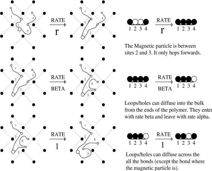
Figure 1: The allowed moves showing the dynamics of a short polymer with a single magnetic bead attached on repton 3, ie between sites 2 and 3. Hernias (excursions out of the confining tube) occur only at the position of the magnetic bead as this is the only part that experiences a force. The velocity of the polymer as a whole is proportional to the density of loops of stored length at the position of the bead.

3 The Currents

Let $n_{i}$ be the binary random variable denoting an occupation of site $i$ by a particle, ie $n_{i}=1$ if site $i$ is occupied and $n_{i}=0$ if it is vacant. For convenience we also introduce $v_{i}=1-n_{i}$. The process described above leads to the following exact evolution equations for the particle density

$$\frac{\partial{\langle n_{1}\rangle}}{\partial t} = {\alpha}\langle v_{1}\rangle-{\beta}\langle n_{1}\rangle+\langle n_{2}\rangle-\langle n_{1}\rangle$$ (1)

$$\frac{\partial{\langle n_{i}\rangle}}{\partial t} = \langle n_{i-1}\rangle-\langle n_{i}\rangle+\langle n_{i+1}\rangle-\langle n_{i}\rangle$$ (2)

$$\frac{\partial{\langle n_{k}\rangle}}{\partial t} = \langle n_{k-1}\rangle-\langle n_{k}\rangle+r\langle v_{k}v_{k+1}\rangle$$ (3)

$$\frac{\partial{\langle n_{k+1}\rangle}}{\partial t} = \langle n_{k+1}\rangle-\langle n_{k}\rangle+r\langle v_{k}v_{k+1}\rangle$$ (4)

$$\frac{\partial{\langle n_{L}\rangle}}{\partial t} = {\alpha}\langle v_{L}\rangle-{\beta}\langle n_{L}\rangle+\langle n_{L-1}\rangle-\langle n_{L}\rangle$$ (5)

This is a non-equilibrium system with a constant steady state current $C$ of particles. As the currents flow from the bond $k,k+1$ it is useful to define $C$, which is proportional to the velocity $V$ of the polymer, as

$$C = {\beta}\langle n_{1}\rangle-{\alpha}\langle v_{1}\rangle$$ (6)

$$C = \langle n_{i+1}\rangle-\langle n_{i}\rangle,\mbox{ for }i<k$$ (7)

$$C = r\langle v_{k}v_{k+1}\rangle$$ (8)

$$C = \langle n_{j}\rangle-\langle n_{j+1}\rangle,\mbox{ for }j>k+1$$ (9)

$$C = {\beta}\langle n_{L}\rangle-{\alpha}\langle v_{L}\rangle$$ (10)

Ignoring correlations at the $k,k+1$ bond - ie approximating $\langle v_{k}v_{k+1}\rangle=\langle v_{k}\rangle\langle v_{k+1}\rangle$ we obtain a simple closed recursion for the steady state particle density and find

$$\langle n_{1}\rangle = \frac{C}{\alpha+\beta}+\frac{\alpha}{\alpha+\beta}$$ (11)

$$\langle n_{L}\rangle = \langle n_{1}\rangle$$ (12)

$$\langle n_{k}\rangle = (k-1)C+\langle n_{1}\rangle$$ (13)

$$\langle n_{k+1}\rangle = (L-k+1)C+\langle n_{L}\rangle$$ (14)

$$\frac{C}{r} = (1-\langle n_{k}\rangle)(1-\langle n_{k+1}\rangle)$$ (15)

Figure 2: Velocity $C$ in lattice units as a function of the position of the attached magnetic bead ($k$) for $L=50$, $r=1$ and $\alpha=\beta=1$ given by mean-field (Eq. (16)) and Monte Carlo simulations. The feature seen here of $C_{mf}{\geq}C_{MC}$ is generic for all values of $r$, the equality holding when the bead is attached at either end [3]. Hence, the mean field solution gives greater dispersion than the exact model and can be used as a bound.

Defining $a=\frac{\beta}{\alpha+\beta}$ and $b=\frac{1}{\alpha+\beta}-1$ we get for the current

$$C = \frac{a(L+2b)+r^{-1}}{2(k+b)(L-k+b)}$$ (16)

$$- \frac{\sqrt{(a(L+2b)+r^{-1})^{2}-4a^{2}(k+b)(L-k+b)}}{2(k+b)(L-k+b)}$$

This gives the drift velocity of the DNA with a magnetic bead attached to repton $k+1$ as a function of the position $k$, the length $N=L+1$ of the DNA and the effective hopping rate $r$ of the tagged repton, see Fig. 2. Not surprisingly the current reaches a maximum if the bead is attached to the center of the DNA and decreases monotonically with increasing distance from the center. In the example given in Fig. 2 the current for the system with a bead attached to the end of the DNA as studied in Ref. [3] is approximately two thirds of the current of the same DNA with a bead attached at the center. As one can see from Monte Carlo simulations, the mean field approximation made above by ignoring the correlation between sites $k,k+1$ leads to a current which is slightly higher than the true current and also enhances the difference in current between chain-end beading and central beading. Therefore, the exact difference between these two extremal situations is actually smaller than given by the expression (16) and the mean-field approximation can be used as a bound on the exact model.

4 Dispersion and Separability

In the following analysis we can for simplicity set $b=0$ corresponding to $\alpha+\beta=1$. This is just a statement about the relative timescales between the boundary and the bulk and will not effect the general type of behaviour. For consistency of notation we express the length dependence of the velocity in terms of $L$ rather than in terms of the number of reptons $N=L+1$. The greatest dispersion for a given $k$ as $L$ is kept constant is between the cases where $k=1$ (at an end) and $k=\frac{L}{2}$ (in the middle). Denoting the current for these two cases by $C_{e}$ and $C_{m}$ respectively we have (with $b=0$)

$$C_{e} = \frac{aL+r^{-1}-\sqrt{(aL+r^{-1})^{2}-4a^{2}(L-1)}}{2(L-1)}$$ (17)

$$C_{m} = \frac{aL+r^{-1}-\sqrt{(aL+r^{-1})^{2}-(aL)^{2}}}{2(\frac{L}{2})^{2}}$$ (18)

If we want to separate polymers of length $L_{1}$ and $L_{2}$ it is important that the dispersion due to differing positions ${\Delta}k$ for a given $L$ of the bead is less than their separability due to their different lengths ${\Delta}L$. Some examples of $C_{e}(L)$ and $C_{m}(L)$ are given in Fig. 3. The velocities seen in this figure are of the same order as those seen in gel electrophoresis, thus fulfilling the first criterion for viability in section 1.

Figure 3: Comparison of $C_{e}$ and $C_{m}$ for different $r$ as $L$ varies with $\alpha=\beta=1$. $C_{m}$ is always the greater in each pair. Good separability occurs when the two lines in a pair $C_{e}$ and $C_{m}$ are close together as this represents low dispersion. Hence, one sees a small $r$ separation regime. The velocities seen here are of the same order as those in constant-field gel electrophoresis.

In order to study the separability due to this dispersion we recall that $C_{e}(L)<C_{m}(L)$. Hence, if we are to separate polymers of length $L_{1}$ and $L_{2}$ where $L_{1}<L_{2}$ we require $\Delta{V}=C_{e}(L_{1})-C_{m}(L_{2})>0$. This inequality gives a lower bound for the length difference of two polymers for which separation is possible.

For extremely small $r\ll(aL)^{-1}$, ie for very immobile beads, one gets $C_{m}\approx C_{e}\approx a^{2}r$. There is no length dispersion due to the position of the bead, but the velocity is very small and length independent. The motion of the DNA is completely determined by the motion of the nearly immobile bead and one has band collapse. It is interesting to note that this situation is analogous to that studied by Aalberts [8] for an extremely bulky end group attached to the DNA under conditions encountered in standard electrophoresis where the force acts on the chain rather than on the bead.

For mobile beads $r\gg(aL)^{-1}$ one gets $L_{2}/L_{1}>2$, making separation possible. Numerically, solutions of this inequality show that it is possible to satisfy the conditions given above also for $r$ of the order $(aL)^{-1}$. In this case one can achieve smaller separation ratios of $L_{2}/L_{1}$. For a detailed numerical analysis, a wide range of $L_{1},L_{2}$ were used and the graphs all showed the same characteristics as seen in Fig. 4 for $L_{1}=400$ and $L_{2}=500$ as a function of $1/r$. There is a regime where $\Delta{V}>0$ and, importantly, also a particular value for $r$ which will maximise the separation. Thus, the second criterion for viablity in section 1 is also satisfied.

Figure 4: Velocity difference for the fastest moving polymer of length 500 and the slowest moving polymer of length 400, $C_{e}(400)-C_{m}(500)$ with $\alpha=\beta=1$. The two polymer fragments are separable for approximately $1/r\geq 100$.

5 Conclusion

To conclude, we have introduced a new variant of the Rubinstein-Duke model to describe the motion of polymers in a gel matrix. We studied the situation where a force acts locally on the polymer and drags it through the gel. Unless one uses extremely immobile beads one finds that even for strong forces there is no band collapse - the drift velocity always depends on the length of the polymer. This is unlike standard (constant field) gel electrophoresis where for sufficiently strong forces long polymers travel with the same velocity and therefore do not separate.

Furthermore, we have shown that the drift velocity of the polymer depends not only on its length, but also on the position where the force acts. As a direct result of this, there is velocity dispersion in a mixture of polymers of the same length if the force acts on different positions in the individual polymers. Nevertheless, we have shown that there is still a regime for which it is possible to separate polymers of different length by letting them move through the gel.

Experimentally, this situation could be realized by attaching magnetic beads to DNA and using a magnetic field gradient [19]. If a bead was made that would attach itself to a commonly occuring chemical group this could be mixed in with the DNA to produce polymers that were tagged at differing positions $k$ from the polymer ends. So for a given length $N$ of polymer there would be a spectrum of configurations with beads attached at different $k$. Some DNA fragments would have no beads, others would have one or more. Once placed in a gel with a magnetic field polymers with no beads will not experience a force and polymers with 2 or more beads will become caught in the gel in hook-like configurations. Such DNA fragments would not move at all. Hence, one only needs to consider the case of polymers that each have a single bead attached at some position $k$ - the situation studied in this paper.

References

- [1] P.G. de Gennes, J. Chem. Phys. 55 (1971) 572.
- [2] S.F. Edwards, Proc. Roy. Soc. London 92 (1967) 9.
- [3] G.T. Barkema and G.M. Schütz, Europhys. Lett. 35 (1996) 139.
- [4] L. Ulanovsky, G. Drouin and W. Gilbert, Nature 343 (1990) 190.
- [5] J. Noolandi, Electrophoresis 13 (1992) 394.
- [6] P. Mayer, G.W. Slater and G. Drouin, Anal. Chem. 66 (1994) 1777.
- [7] A. Adjari, F. Brochard-Wyart, P.G. de Gennes and J.L. Viovy, J. Phys. II France 5 (1995) 491.
- [8] D. Aalberts, Phys. Rev. Lett. 75 (1995) 4544.
- [9] M. Rubinstein, Phys. Rev. Lett. 59 (1987) 1946.
- [10] T.A.J. Duke, Phys. Rev. Lett. 62 (1989) 2877.
- [11] B. Widom, J.L. Viovy and A.D. Défontaines, J.Phys. I France 1 (1991) 1759.
- [12] J.M.J. van Leeuwen, J. Phys. I France 1 (1991) 1675.
- [13] J.M.J. van Leeuwen and A. Kooiman, Physica A 184 (1992) 79.
- [14] M. Prähofer, University of Munich thesis (1994); M. Prähofer and H. Spohn, to appear in Physica A.
- [15] J.A. Leegwater and J.M.J. van Leeuwen, Phys. Rev. E 52 (1995) 2753.
- [16] A.B. Kolomeisky and B. Widom, Physica A 229 (1996) 53.
- [17] G.T. Barkema, J.F. Marko and B. Widom, Phys. Rev. E 49 (1994) 5303.
- [18] G.T. Barkema, C. Caron, and J.F. Marko, Biopolymers 38 (1996) 665.
- [19] B.-I. Haukanes and C. Kvam, Biotechnology 11 (1993) 60.