Aperiodic spin chain in the mean-field approximation

Abstract

Surface and bulk critical properties of an aperiodic spin chain are investigated in the framework of the $\phi^{4}$ phenomenological Ginzburg-Landau theory. According to Luck’s criterion, the mean field correlation length exponent $\nu=1/2$ leads to a marginal behaviour when the wandering exponent of the sequence is $\omega=-1$. This is the case of the Fibonacci sequence that we consider here. We calculate the bulk and surface critical exponents for the magnetizations, critical isotherms, susceptibilities and specific heats. These exponents continuously vary with the amplitude of the perturbation. Hyperscaling relations are used in order to obtain an estimate of the upper critical dimension for this system.

1 Introduction

The discovery of quasicrystals [1] has focused considerable interest on quasiperiodic or, more generally, aperiodic systems [2]. In the field of critical phenomena, due to their intermediate situation between periodic and random systems, aperiodic models have been intensively studied (for a review, see [7]). Furthermore, aperiodic multilayers are experimentally feasible and should build a new class of artificial structures exhibiting interesting bulk and surface properties. Although aperiodic superlattices have already been worked out by molecular beam epitaxy [8], nothing has been done experimentally up to now from the point of view of critical phenomena. In the perspective of possible future experimental studies in this context, it seems an interesting and challenging problem to complete our understanding through a mean field theory approach. Surface critical behaviour has indeed been intensively investigated on the basis of the Ginzburg-Landau theory [9] in the seventies [11]. This led to a classification of the transitions which may occur at the surface and to the derivation of scaling laws between surface and bulk critical exponents [18] (for a review, see [24]). These early papers are known as an important stage in the further developments of surface critical phenomena.

Seen from the side of critical phenomena, the universal behaviour of aperiodically perturbed systems is now well understood since Luck proposed a relevance-irrelevance criterion [25, 26]. The characteristic length scale in a critical system is given by the correlation length and as in the Harris criterion for random systems [28], the strength of the fluctuations of the couplings on this scale determines the critical behaviour. An aperiodic perturbation can thus be relevant, marginal or irrelevant, depending on the sign of a crossover exponent involving the correlation length exponent $\nu$ of the unperturbed system and the wandering exponent $\omega$ which governs the size-dependence of the fluctuations of the aperiodic couplings [29]. In the light of this criterion, the results obtained in early papers, mainly concentrated on the Fibonacci [31] and the Thue-Morse [39] sequences, found a consistent explanation, since, resulting from the bounded fluctuations, a critical behaviour which resembles the periodic case was found for the Ising model in two dimensions.

In the last years, much progress have been made in the understanding of the properties of marginal and relevant aperiodically perturbed systems. Exact results for the $2d$ layered Ising model and the quantum Ising chain have been obtained with irrelevant, marginal and relevant aperiodic perturbations [41, 49]. The critical behaviour is in agreement with Luck’s criterion leading to essential singularities or first-order surface transition when the perturbation is relevant and power laws with continuously varying exponents in the marginal situation with logarithmically diverging fluctuations. A strongly anisotropic behaviour has been recognized in this latter situation [50, 52]. Marginal surface perturbations have also been studied with the Fredholm sequence [53] and conformal aspects have been discussed [54].

In the present paper, we continue our study of marginal sequences. The case of the Fibonacci sequence, which leads to irrelevant behaviour in the Ising model, should exhibit non universal properties within mean field approach according to the Luck criterion and it has not yet been studied in this context. The article is organized as follows: in section 2, we present the phenomenological Ginzburg-Landau theory on a discrete lattice with a perturbation following a Fibonacci sequence and we summarize the scaling arguments leading to Luck’s criterion, then we discuss the definitions of both bulk and surface thermodynamic quantities. We consider magnetic properties in section 3. Both bulk and surface quantities are computed numerically, leading to the values of the corresponding critical exponents. In section 4, we discuss the thermal properties and eventually in section 5, we discuss the upper critical dimension of the model.

2 Discrete Ginzburg-Landau equations for a Fibonacci aperiodic perturbation

2.1 Landau expansion and equation of state on a one-dimensional lattice

Let us first review briefly the essentials of the Ginzburg-Landau theory formulated on a discrete lattice. We consider a one-dimensional lattice of $L$ sites with a lattice spacing $\ell$ and free boundary conditions. The critical behaviour would be the same as in a $d-$dimensional plate of thickness $L\ell$ with translational invariance along the $d-1$ directions perpendicular to the chain and extreme axial anisotropy which forces the magnetic moments to keep a constant direction in the plane of the plate. We investigate the critical properties of an aperiodically distributed perturbation within the framework of a $\phi^{4}$ phenomenological Landau theory [56]. The underlying assumption in this approach is based on the following expansion of the bulk free energy density

$$f_{b}\{\phi_{j}\}={1\over 2}\mu_{j}\phi_{j}^{2}+{1\over 4}g\phi_{j}^{4}-H\phi_{j}+{1\over 2}c\left({\phi_{j+1}-\phi_{j}\over\ell}\right)^{2},$$ (1)

where the aperiodic perturbation of the coupling constants is determined by a two-digits substitution rule and enters the $\phi^{2}$ term only. A dimensional analysis indeed shows that the deviation from the critical temperature, $\mu$, is the relevant scaling field which has to be modified by the perturbation. The free energy of the whole chain is thus given by

$$F[\phi_{j}]=\sum_{j}f_{b}\{\phi_{j}\},$$ (2)

and the spatial distribution of order parameter satisfies the usual functional minimization:

$$\delta F[\phi_{j}]=F[\phi_{j}+\delta\phi_{j}]-F[\phi_{j}]=0.$$ (3)

One then obtains the coupled discrete Ginzburg-Landau equations:

$$\mu_{j}\phi_{j}+g\phi_{j}^{3}-H-{c\over\ell^{2}}(\phi_{j+1}-2\phi_{j}+\phi_{j-1})=0.$$ (4)

The coefficients $\mu_{j}$ depend on the site location and are written as

$$\mu_{j}=k_{B}T-(zJ-Rf_{j})=a_{0}\left(1-{1\over\theta}+rf_{j}\right),$$ (5)

where $J$ is the exchange coupling between neighbour sites in the homogeneous system, $z$ the lattice coordination and $f_{j}$ the aperiodically distributed sequence of $0$ and $1$. The prefactor $a_{0}=k_{B}T$ is essentially constant in the vicinity of the critical point, and the temperature $\theta$ is normalized relatively to the unperturbed system critical temperature: $\theta=k_{B}T/zJ$. In the following, we will also use the notation $\mu=1-1/\theta$. In order to obtain a dimensionless equation, let us define $\phi_{j}=m_{j}\sqrt{a_{0}/g}$ leading to the following non-linear equations for the $m_{j}$’s:

$$(\mu+rf_{j})m_{j}+m_{j}^{3}-h-(m_{j+1}-2m_{j}+m_{j-1})=0,$$ (6)

with boundary conditions

$$(\mu+rf_{1})m_{1}+m_{1}^{3}-h-(m_{2}-2m_{1})=0,$$ (7a)

$$(\mu+rf_{L})m_{L}+m_{L}^{3}-h-(-2m_{L}+m_{L-1})=0.$$ (7b)

Here, the lengths are measured in units $\ell=\sqrt{c/a_{0}}$ and $h=H\sqrt{g/a_{0}^{3}}$ is a reduced magnetic field.

One can point out the absence of specific surface term in the free energy density. The surface equations for the order parameter profile simply keep the bulk form with the boundary conditions $m_{0}=m_{L+1}=0$ and our study will only concern ordinary surface transitions [24].

2.2 Fibonacci perturbation and Luck’s criterion

The Fibonacci perturbation considered below may be defined as a two digits substitution sequence which follows from the inflation rule

$$0\rightarrow S(0)=01,\quad 1\rightarrow S(1)=0,$$ (8)

leading, by iterated application of the rule on the initial word $0$, to successive words of increasing lengths:

$$\begin{array}[]{llllllll}0&&&&&&&\\ 0&1&&&&&&\\ 0&1&0&&&&&\\ 0&1&0&0&1&&&\\ 0&1&0&0&1&0&1&0\\ .&.&.&&&&&\\ \end{array}$$ (9)

It is now well known that most of the properties of such a sequence can be characterized by a substitution matrix whose elements $M_{ij}$ are given by the number $n_{i}^{S(j)}$ of digits of type $i$ in the substitution $S(j)$ [25, 29]. In the case of the Fibonacci sequence, this yields

$$\underline{\underline{\bf M}}=\left(\begin{array}[]{cc}n_{0}^{S(0)}&n_{0}^{S(1)}\\ n_{1}^{S(0)}&n_{1}^{S(1)}\\ \end{array}\right)=\left(\begin{array}[]{cc}1&1\\ 1&0\\ \end{array}\right).$$ (10)

The largest eigenvalue of the substitution matrix is given by the golden mean $\Lambda_{1}={1+\sqrt{5}\over 2}$ and is related to the length of the sequence after $n$ iterations, $L_{n}\sim\Lambda_{1}^{n}$, while the second eigenvalue $\Lambda_{2}=-1/\Lambda_{1}$ governs the behaviour of the cumulated deviation from the asymptotic density of modified couplings $\rho_{\infty}=1-{2\over\sqrt{5}+1}$:

$$\sum_{j=1}^{L}(f_{j}-\bar{f})=n_{L}-\rho_{\infty}L\sim\mid\Lambda_{2}\mid^{n}\sim(\Lambda_{1}^{\omega})^{n},$$ (11)

where we have introduced the sum $n_{L}=\sum_{j=1}^{L}f_{j}$ and the wandering exponent

$$\omega={\ln\mid\Lambda_{2}\mid\over\ln\Lambda_{1}}=-1.$$ (12)

When the scaling field $\mu$ is perturbed as considered in the previous section,

$$\mu_{j}=a_{0}\left(\mu+rf_{j}\right),$$ (13)

the cumulated deviation of the couplings from the average at a length scale $L$

$$\overline{\delta\mu}(L)={1\over L}\sum_{j=1}^{L}(\mu_{j}-\bar{\mu})={1\over L}a_{0}r(n_{L}-\rho_{\infty}L)$$ (14)

behaves with a size power law:

$$\overline{\delta\mu}(L)\sim L^{\omega-1},$$ (15)

and induces a shift in the critical temperature $\overline{\delta t}\sim\xi^{\omega-1}$ to be compared with the deviation $t$ from the critical temperature:

$${\overline{\delta t}\over t}\sim t^{-(\nu(\omega-1)+1)}.$$ (16)

This defines the crossover exponent $\phi=\nu(\omega-1)+1$. When $\phi=0$, the perturbation is marginal: it remains unchanged under a renormalization transformation, and the system is thus governed by a new perturbation-dependent fixed point.

A perturbation of the parameters $g$ or $c$ entering the Landau expansion (1) would be irrelevant.

2.3 Bulk and surface thermodynamic quantities

In the following, we discuss both bulk and surface critical exponents and scaling functions. We deal with the surface and boundary magnetizations $m_{s}$ and $m_{1}$, surface and boundary susceptibilities $\chi_{s}$ and $\chi_{1}$, and surface specific heat $C_{s}$. All these quantities can be expressed as derivatives of the surface free energy density $f_{s}$ [24] (see table 1).

Table 1: Bulk and surface thermodynamic quantities in terms of the bulk $f_{b}$ and surface $f_{s}$ free energy densities. $h$ and $h_{1}$ are bulk and surface magnetic fields respectively and $t$ is the reduced temperature.

magnetization				susceptibility			specific heat
bulk	surface		bulk	surface		bulk	surface
$m_{b}=-{\partial f_{b}\over\partial h}$	$m_{s}=-{\partial f_{s}\over\partial h}$		$\chi_{b}=-{\partial^{2}f_{b}\over\partial h^{2}}$	$\chi_{s}=-{\partial^{2}f_{s}\over\partial h^{2}}$		$C_{b}=-{\partial^{2}f_{b}\over\partial t^{2}}$	$C_{s}=-{\partial^{2}f_{s}\over\partial t^{2}}$
	$m_{1}=-{\partial f_{s}\over\partial h_{1}}$			$\chi_{1}=-{\partial^{2}f_{s}\over\partial h\partial h_{1}}$
				$\chi_{11}=-{\partial^{2}f_{s}\over\partial h_{1}^{2}}$

While there is no special attention to pay to these definitions in a homogeneous system, they have to be carefully rewritten in the perturbed model that we consider here. First of all, we shall focus on local quantities such as the boundary magnetization $m_{1}$ or the local bulk magnetization $m_{(n-1)}$, defined, for a chain of size $L_{n}$ obtained after $n$ substitutions, by the order parameter at position $L_{n-1}$. This definition leads to equivalent sites for different chain sizes (see figure 1).

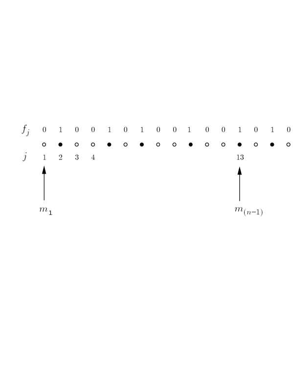
Figure 1: Fibonacci chain of 21 sites. The local bulk magnetization, for a chain of $L_{n}$ sites obtained after $n$ iterations of the substitution rule is computed on the site $L_{n-1}$, here site 13.

In addition to these local quantities, one may also calculate both surface and mean bulk magnetizations ($m_{s}$ and $m_{b}$ respectively), which should be interesting from an experimental point of view since any experimental device would average any measurement over a large region compared to microscopic scale. In order to keep symmetric sites with respect to the middle of the chain, and to avoid surface effects, the mean bulk magnetization $m_{b}$ is defined by averaging over $L_{n-2}$ sites around the middle for a chain of size $L_{n}$.

$$m_{b}={1\over L_{n-2}}\sum_{j\in L_{n-2}}m_{j}.$$ (17)

We checked numerically that one recovers the same average as for a chain of size $L_{n-2}$ with periodic boundary conditions. Following Binder [24], for a film of size $L_{n}$ with two free surfaces, the surface magnetization is then defined by the deviation of the average magnetization $\langle m_{j}\rangle$ over the whole chain from the bulk mean value:

$$m_{s}={1\over 2}\left(m_{b}-{1\over L_{n}}\sum_{j=1}^{L_{n}}m_{j}\right).$$ (18)

A graphical description can be found in figure 2.

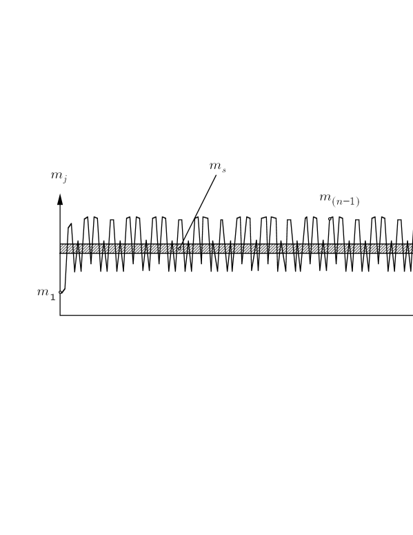
Figure 2: Typical shape of the order parameter profile for a perturbed system, showing the boundary and local bulk magnetizations $m_{1}$ and $m_{(n-1)}$, and the average values $m_{b}$ and $\langle m_{j}\rangle$

In the following, we shall use brackets for the averages over the finite system, taking thus surface effects into account. In the same way, the bulk free energy density in table 1 has to be understood as:

$$f_{b}={1\over L_{n-2}}\sum_{j\in L_{n-2}}f_{b}\{m_{j}\}$$ (19)

while the surface free energy density $f_{s}$ is defined as the excess from the average bulk free energy

$$F=\sum_{j=1}^{L_{n}}f_{b}\{m_{j}\}=L_{n}\langle f_{b}\rangle=L_{n}f_{b}+2f_{s}.$$ (20)

3 Magnetic properties

3.1 Order parameter profile and critical temperature

The order parameter profile is determined numerically by a Newton-Raphson method, starting with arbitrary values for the initial trial profile ${m_{j}}$. Equation (6) provides a system of $L$ coupled non-linear equations

$$G_{i}(m_{1},m_{2},\dots,m_{L})=0,\quad i=1,2,\dots,L$$ (21)

for the components of the vector $\vec{m}=(m_{1},m_{2},\dots,m_{L})$, which can be expanded in a first order Taylor series:

$$G_{i}(\vec{m}+\delta\vec{m})=G_{i}(\vec{m})+\sum_{j=1}^{L}{\partial G_{i}\over\partial m_{j}}\delta m_{j}+O(\delta\vec{m}^{2}).$$ (22)

A set of linear equations follows for the corrections $\delta\vec{m}$

$$\sum_{j=1}^{L}{\partial G_{i}\over\partial m_{j}}\delta m_{j}=-G_{i}(\vec{m})$$ (23)

which moves each function $G_{i}$ closer to zero simultaneously. This technique is known to provide a fast convergence towards the exact solution. Typical examples of the profile obtained for the Fibonacci perturbation are shown on figure 3.

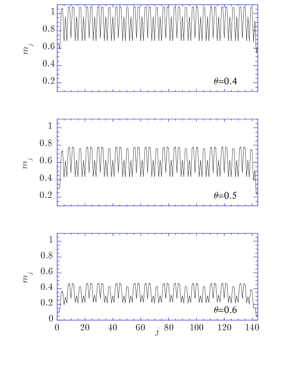
Figure 3: Order parameter profiles for a perturbation $r=2$ and three values of the temperature below the critical point. The size of the chain is $L=144$.

The magnetization profile decreases as the temperature is increased and vanishes for some size-dependent effective value of the critical temperature $\mu_{c}(L)=1-(\theta_{c}(L))^{-1}$. This value may be obtained through a recursion relation deduced from the equation of state. In the high temperature phase, when $h=0$, equation (6) can be rewritten as a homogeneous system of linear equations:

$$\underline{\underline{\bf G}}\vec{m}=\left(\begin{array}[]{cccccc}\alpha_{1}&-1&0&0&\dots&0\\ -1&\alpha_{2}&-1&0&\dots&0\\ 0&-1&\alpha_{3}&-1&\ddots&\vdots\\ \vdots&\vdots&\ddots&\alpha_{j}&\ddots&\vdots\\ 0&\dots&0&0&-1&\alpha_{L}\\ \end{array}\right)\left(\begin{array}[]{c}m_{1}\\ m_{2}\\ \vdots\\ \vdots\\ m_{L}\\ \end{array}\right)=0,$$ (24)

where $\alpha_{j}=2+\mu+rf_{j}$. If the determinant $D_{L}(\mu)=\hbox{\rm Det}\ \underline{\underline{\bf G}}(\mu)$ is not vanishing, the null vector ${\vec{m}}=\vec{0}$ provides the satisfying unique solution for the high temperature phase. The critical temperature is then defined by the limiting value $\mu_{c}(L)$ which allows a non-vanishing solution for ${\vec{m}}$, i.e. $D_{L}(\mu_{c})=0$. Because of the tridiagonal structure of the determinant, the following recursion relation holds, for any value of $\mu$:

$$D_{L}(\mu) = \alpha_{L}D_{L-1}(\mu)-D_{L-2}(\mu),$$ (25a)

$$D_{0}(\mu) = 1,$$ (25b)

$$D_{1}(\mu) = \alpha_{1}.$$ (25c)

Thus we can obtain $\mu_{c}(L)$ for different sizes $L$ from 144 to 46368 and estimate the asymptotic critical point by an extrapolation to infinite size. This technique allows a determination of the critical temperature with an absolute accuracy in the range $10^{-7}$ to $10^{-9}$ depending on the value of the amplitude $r$.

3.2 Surface and bulk spontaneous magnetization behaviours

The boundary magnetization $m_{1}$ vanishes at the same temperature than the profile itself. First of all, the influence of finite size effects [57] has to be studied. This is done by the determination of the profiles for different chains of lengths given by the successive sizes of the Fibonacci sequence $L=1,2,3,5,8,13,21,34\dots$ The boundary and bulk magnetization in zero magnetic field are shown on figure 4 on a log-log scale.

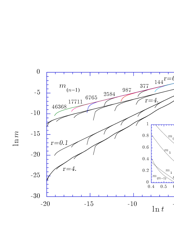
Figure 4: Log-Log plot of the bulk and boundary magnetization v.s. the reduced temperature $t=\mu_{c}-\mu$ for two values of the aperiodic amplitude $r$ and for different sizes of the chain from 144 to 46368. Finite-size effects occur when the curves deviate from the asymptotic straight line. The insert shows the behaviour of the magnetization with the temperature.

The finite size effects appear in the deviation from the straight line asymptotic behaviour. These effects are not too sensitive, as it can be underscored by considering the deviation of the curve for a size $L=17711$, which occurs around $t=\mu_{c}-\mu\simeq 10^{-7}$, i.e. very close to the critical point.

The expected marginal behaviour is furthermore indicated by the variation of the slopes with the aperiodic modulation amplitude $r$ and is more noticeable for the boundary magnetization than in the case of the bulk.

A more detailed inspection of these curves also shows oscillations resulting from the discrete scale invariance [58] of the system and the asymptotic magnetization can thus be written

$$m(t)=t^{\beta}\tilde{m}(t^{-\nu})$$ (26)

where $\tilde{m}(t^{-\nu})$ is a log-periodic scaling function of its argument. We make use of this oscillating behaviour to obtain a more precise determination of the critical temperature (in the range $10^{-11}$ to $10^{-12}$) and of the values of the bulk and surface exponents by plotting the rescaled magnetization $mt^{-\beta}$ as a function of $\ln t^{-\nu}$ as shown on figure 5 in the case of the first layer.

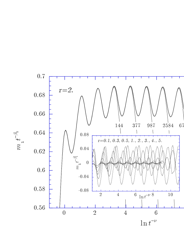
Figure 5: Periodic oscillations of the rescaled boundary magnetization $m_{1}t^{-\beta_{1}}$ v.s. $\ln t^{-\nu}$. The deviation from the oscillating behaviour for large values of the correlation length $t^{-\nu}$ is due to finite-size effects. The insert shows the oscillations of the rescaled boundary magnetization for different values of $r$ after substraction of a constant amplitude.

The values of $\mu_{c}$ and $\beta_{1}$ that we consider suitable are the ones which allow an oscillating behaviour for the widest interval in the variable $\ln t^{-\nu}$. A modification of the boundary exponent $\beta_{1}$ would change the average slope of the oscillating regime. This could be due to corrections to scaling, but, if such corrections really existed, they should cancel in this range of temperatures (in the oscillating regime, $t$ goes to values as small as $10^{-9}$). The other parameter, $\mu_{c}$, modifies the number of oscillations and we have choosen a value leading to the largest number of such oscillations. A poor determination of the critical point $\mu_{c}^{\prime}=\mu_{c}+\Delta\mu_{c}$ would indeed artificially introduce a correction to scaling term, since $t^{\beta}=(t^{\prime}+\Delta\mu_{c})^{\beta}\sim t^{\prime\beta}\left(1+\beta\frac{\Delta\mu_{c}}{t^{\prime}}\right)$.

Table 2: Numerical values of the critical temperature and the magnetic exponents for the surface and bulk magnetizations. The figure in brackets gives the uncertainty on the last digit.

		surface				bulk
$r$	$\theta_{c}$	$\beta_{1}$	$\beta_{L}$	$\beta_{s}$		$\beta_{(n-1)}$	$\beta_{b}$
.1	.963977634341 (5)	1.00036 (2)	——	.0002 (2)		.500087 (1)	.5002 (2)
.2	.93187679929 (2)	1.00146 (2)	1.0015 (1)	——		.50033 (1)	——
.3	.90314503363 (2)	1.0034 (1)	1.0034 (1)	——		.50072 (6)	——
.5	.85404149087 (2)	1.0092 (1)	——	.0094 (2)		.50187 (1)	.505 (1)
.8	.796437160887 (5)	1.02214 (2)	——	.0216 (2)		.50419 (2)	——
1.	.76600595095 (2)	1.0327 (1)	——	.0302 (2)		.505777 (2)	.516 (1)
1.5	.70902241601 (2)	1.0621 (1)	——	——		.50943 (1)	——
2.	.67010909237 (2)	1.0913 (1)	——	.087 (1)		.51186 (3)	.538 (1)
2.5	.64234629279 (2)	1.1178 (1)	——	——		.51294 (1)	——
3.	.621796760462 (5)	1.1410 (1)	1.1410 (1)	.133 (1)		.5132 (1)	.555 (1)
3.5	.60610567508 (2)	1.1602 (1)	——	——		.51327 (4)	——
4.	.593804120472 (5)	1.1766 (1)	——	.1692 (4)		.5130 (1)	.563 (1)
4.5	.58394117369 (2)	1.1904 (1)	——	——		.5122 (1)	——
5.	.5758805295248 (5)	1.2026 (1)	——	.195 (1)		.51125 (2)	.567 (1)

The corresponding values of $\theta_{c}$, $\beta_{1}$ and $\beta_{(n-1)}$ are given for several values of the perturbation amplitude $r$ in table 2. The critical exponent associated to the right surface ($m_{L}$) of the Fibonacci chain has also been computed for different values of $r$ for the largest chain size. It gives, with a good accuracy, the same value as for the left surface ($m_{1}$) as it can be seen by inspection in the table. The aperiodic sequence is indeed the same, seen from both ends, if we forget the last two digits.

Furthermore, the profiles of figure 3 clearly show that the sites of the chain are not all equivalent and the magnetization profiles can be locally rescaled with different values of the exponents depending on the site [52]. Thus, after the local quantities, the computation of the surface and mean bulk magnetizations enable us to determine the critical exponents respectively written $\beta_{s}$ and $\beta_{b}$ and given in table 2.

From our values, one obviously recovers the usual unperturbed ordinary transition values of the exponents when the perturbation amplitude goes to zero.

3.3 Susceptibility and critical isotherm

Taking account of a non vanishing bulk magnetic field in equations (6) and (7), one can compute the magnetization in a finite field and then deduce the critical isotherms exponents $\delta_{(n-1)}$ and $\delta_{1}$ from the behaviours of the local magnetizations $m_{(n-1)}$ and $m_{1}$ with respect to $h$:

$$m_{(n-1)}\sim h^{1/\delta_{(n-1)}},\hskip 25.0ptm_{1}\sim h^{1/\delta_{1}},\hskip 25.0ptt=0.$$ (27)

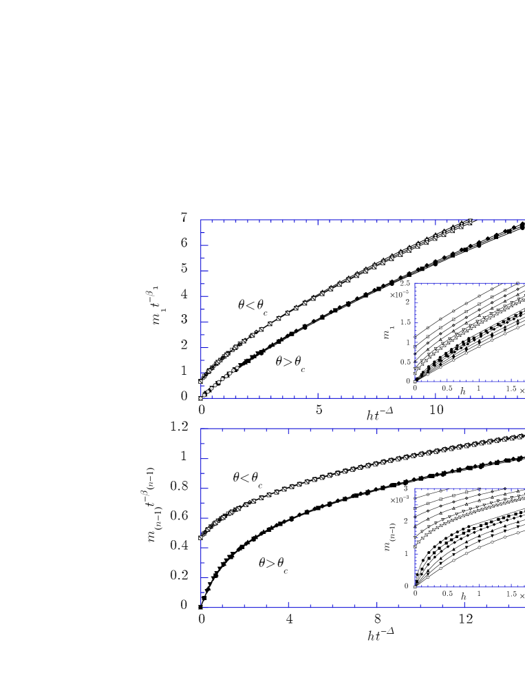
Figure 6: Rescaled equations of state for the boundary and bulk magnetization for $r=2$. The values of the temperature are $\theta=0.670090$, $0.670094$, $0.670097$, $0.670100$, $0.670103$, $0.670105$ below $\theta_{c}$ and $0.670111$, $0.670113$, $0.670115$, $0.670118$, $0.670121$, $0.670125$ above $\theta_{c}$. Top: scaling functions $f_{m_{1}}^{\pm}$, the insert shows the boundary magnetization as a function of the bulk magnetic field. Bottom: same as above for the local bulk magnetization.

This time, a direct log-log plot allows a precise determination of the exponents and the rescaled equation of state confirms the validity of the estimate since we obtain a good data collapse. In the case of the boundary magnetization, the scaling assumption takes the following form under rescaling by an arbitrary factor $b$:

$$m_{1}(t,h)=b^{-\beta_{1}/\nu}m_{1}(b^{y_{t}}t,b^{y_{h}}h),$$ (28)

where $y_{t}$ is given by the inverse of the correlation length exponent $y_{t}=1/\nu$ and the value of the magnetic field anomalous dimension $y_{h}$ follows the requirements of (27): $y_{h}=\beta_{1}\delta_{1}/\nu=\beta\delta/\nu$. The choice $b=t^{-\nu}$ for the rescaling factor then leads to a universal behaviour expressed in terms of a single scaled variable:

$$m_{1}(t,h)=t^{\beta_{1}}f_{m_{1}}^{\pm}(ht^{-\Delta})$$ (29)

where $\Delta=\beta_{1}\delta_{1}$ is the so-called gap exponent, $f_{m_{1}}^{\pm}$ is a universal scaling function and $\pm$ refers to the two phases $\theta>\theta_{c}$ and $\theta<\theta_{c}$. This may then be checked by a plot of $m_{1}t^{-\beta_{1}}$ v.s. $ht^{-\Delta}$ shown on figure 6 and the same type of universal function have been obtained for the local bulk site $m_{(n-1)}t^{-\beta_{(n-1)}}=f_{m_{(n-1)}}^{\pm}(ht^{-\Delta})$. The values of $\delta_{1}$ and $\delta_{(n-1)}$ are given in table 3.

Table 3: Numerical values of the critical exponents associated to the critical isotherms and the susceptibilities. $\gamma_{b}$ and $\delta_{b}$ correspond to the behaviour of the mean bulk magnetization $m_{b}$. The figure in brackets gives the uncertainty on the last digit.

	surface					bulk
$r$	$\gamma_{1}$	$\delta_{1}$	$\gamma_{s}$	$\delta_{s}$		$\gamma_{(n-1)}$	$\delta_{(n-1)}$	$\gamma_{b}$	$\delta_{b}$
.1	.5013 (2)	1.5024 (2)	1.498 (1)	——		.9997 (1)	2.9989 (1)	1.0005 (1)	——
.2	.5006 (2)	1.5004 (2)	——	——		.9993 (2)	2.9972 (3)	——	——
.3	.4992 (2)	1.4977 (2)	——	——		.9993 (2)	2.9949 (9)	——	——
.5	.4958 (2)	1.4901 (2)	1.493 (1)	312 (11)		.9989 (2)	2.9895 (9)	.99790 (2)	2.98136 (2)
.8	.487 (1)	1.4751 (3)	1.486 (1)	85 (2)		.9986 (3)	2.981 (2)	——	——
1.	.4796 (2)	1.4641 (2)	1.480 (2)	53 (1)		.9985 (4)	2.9744 (9)	.99253 (2)	2.93144 (2)
1.5	.4568 (2)	1.4378 (4)	——	——		.9988 (7)	2.963 (3)	——	——
2.	.4316 (2)	1.4135 (1)	1.438 (2)	16.37 (2)		.999 (2)	2.9571 (1)	.9792 (1)	2.82375 (3)
2.5	.412 (1)	1.3845 (6)	——	——		.9992 (9)	2.954 (2)	——	——
3.	.388 (1)	1.3484 (6)	1.394 (2)	11.2 (2)		.9988 (6)	2.952 (2)	.9660 (1)	2.7513 (2)
3.5	.372 (1)	1.3108 (5)	——	——		.9986 (5)	2.949 (2)	——	——
4.	.354 (1)	1.2989 (4)	1.360 (2)	10.01 (5)		.9988 (8)	2.948 (2)	.9619 (5)	2.6976 (3)
4.5	.341 (1)	1.2571 (2)	——	——		.999 (1)	2.950 (2)	——	——
5.	.328 (1)	1.2467 (6)	1.330 (2)	8.3 (4)		.999 (2)	2.953 (2)	.9514 (2)	2.65938 (2)

The behaviours of $m_{s}$ and $m_{b}$ with $h$ at the critical point lead to the values of $\delta_{s}$ and $\delta_{b}$, also listed in table 3. We can point out the low accuracy in the determination of $\delta_{s}$ since the slope of the log-log plot of $m_{s}$ v.s. $h$ is quite small when $r$ reaches the unperturbed value $r=0$.

The derivative of equation (28) with respect to the bulk magnetic field $h$ defines the boundary susceptibility $\chi_{1}$ which diverges as the critical point is approached with an exponent $\gamma_{1}$. Numerically, the boundary magnetization is calculated for several values of the bulk magnetic field (of the order of $10^{-9}$), and $\chi_{1}$ follows a finite difference derivation. The bulk local susceptibility $\chi_{(n-1)}$ may be obtained in the same way. Log-periodic oscillations also occur in these quantities and the determination of the exponents can be done in the same way as in the previous section for the magnetization. Again, the accuracy of the result is confirmed by the rescaled curves for the susceptibilities, for example $\chi_{(n-1})t^{\gamma_{(n-1)}}=f_{\chi_{(n-1)}}^{\pm}(ht^{-\Delta})$ shown on figure 7 exhibits a good data collapse on two universal curves for $\theta<\theta_{c}$ and $\theta>\theta_{c}$.

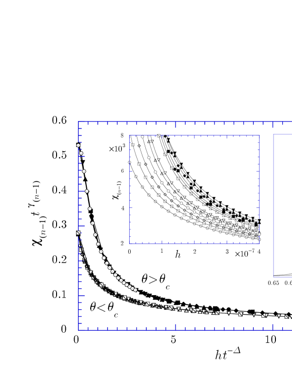
Figure 7: Rescaled bulk susceptibility giving the behaviour of the universal functions $f_{\chi_{(n-1)}}^{\pm}$ below and above $\theta_{c}$ for $r=2$. The values of the temperature are the same as in figure 6. The inserts show the behaviours of $\chi_{(n-1)}$ as a function of $h$ for the same temperatures (left), and the singularities of both $\chi_{(n-1)}$ and $\chi_{1}$ in zero magnetic field as a function of $\theta$ (right).

The values of the exponents are given in table 3 which presents also $\gamma_{s}$ and $\gamma_{b}$, associated to the surface and average bulk magnetization field derivatives.

4 Specific heat

According to the definitions of section 2, the surface and bulk free energies are also defined as follows:

$$F_{s}={1\over 2}(F_{FBC}-F_{PBC}),$$ (30a)

$$F_{b}=F_{PBC}.$$ (30b)

where $F_{FBC}$ and $F_{PBC}$ denote the total free energies of aperiodic chains with free and periodic boundary conditions respectively and are obtained numerically using equations (19) and (20).

The expected singular behaviours of the free energy densities

$$f_{s} (t,h)=t^{2-\alpha_{s}}f_{s}(ht^{-\Delta}),$$ (31a)

$$f_{b} (t,h)=t^{2-\alpha_{b}}f_{b}(ht^{-\Delta}),$$ (31b)

where the dependence of $f_{s}$ with the local magnetic surface field $h_{1}$ has been omitted since we always consider the case $h_{1}=0$, lead to the surface and bulk specific heat exponents. The values of $\alpha_{s}$ and $\alpha_{b}$ are simply deduced from the slopes of the log-log plots of $f_{s}$ and $f_{b}$ v.s. $t$.

In figure 8, we show the bulk free energy density amplitude $f_{b}t^{\alpha_{b}-2}$ as a function of $\ln t^{-\nu}$ for $r=2$. It exhibits the same type of oscillating behaviour than the rescaled magnetisation of figure 5.

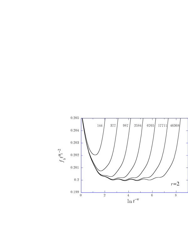
Figure 8: Rescaled bulk free energy density $f_{b}t^{\alpha_{b}-2}$ v.s. $\ln t^{-\nu}$ for $r=2$. The amplitude of the bulk free energy density exhibits log-periodic oscillations.

The surface and bulk specific heat exponents are collected in table 4. The bulk specific heat discontinuity of the homogeneous system is washed out in the perturbed system, since $\alpha_{b}<0$.

Table 4: Numerical values of the specific heat critical exponents. The figure in brackets gives the uncertainty on the last digit.

• $r$	$\alpha_{s}$	$\alpha_{b}$
  .1	0.51496 (7)	-0.00031 (1)
  .5	0.50112 (5)	-0.00733 (1)
  .8	0.48448 (5)	-0.01709 (1)
  1.	0.47075 (4)	-0.02462 (1)
  2.	0.40265 (1)	-0.05924 (1)
  3.	0.35077 (4)	-0.07813 (1)
  4.	0.31516 (3)	-0.08579 (1)
  5.	0.28935 (6)	-0.08805 (1)

5 Discussion

We have calculated numerically several surface and bulk critical exponents for a marginal aperiodic system within mean field theory. The marginal aperiodicity leads to exponents which vary continuously with the amplitude of the perturbation $r$. The variations of these exponents are shown on figure 9 as a function of $r$.

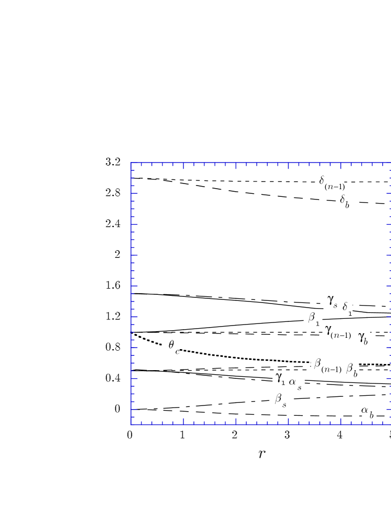
Figure 9: Variations of the surface and bulk exponents with the perturbation amplitude $r$ (boundary exponents: ——, surface: — $\cdot$ —, local bulk: —-, mean bulk: – – –).

The comparison in table 2 between the bulk exponent $\beta_{b}$ and the local one $\beta_{(n-1)}$ clearly shows that it is no longer possible, in this aperiodic system, to define a unique bulk exponent, as it was already suggested by the possibility of a local rescaling of the profiles with position-dependent exponents which suggests a multiscaling behaviour. A constant value $y_{t}=1/\nu$ is consistent with continuously varying exponents, in order to keep a vanishing crossover exponent which ensures that the marginality condition remains valid for any value of the aperiodicity amplitude $r$. For $y_{h}$ on the other hand, there is no such reason. From this point of view, equations like (28) are not exact since a unique field anomalous dimension $y_{h}$ has no real significance. It follows that the universal functions in figure 6 and figure 7 only give an approximate picture of the scaling behaviour in this system, since they involve the gap exponent $\Delta=y_{h}/y_{t}$. The good data collapse has to be credited to the weak variation of the exponents with the perturbation amplitude $r$.

On the other hand, the scaling laws involving the dimension of the system are satisfied in mean field theory with a value of $d$ equal to the upper critical dimension $d^{*}$. As for the $2d$ Ising model with a marginal aperiodicity [50, 52], one expects a strongly anisotropic behaviour in the Gaussian model. It yields a continuous shift of the upper critical dimension with the pertubation amplitude, $d^{*}(r)$, since the value $d^{*}=4$ for a critical point in the homogeneous $\phi^{4}$ theory follows Ginzburg’s criterion for an isotropic behaviour. Hyperscaling relations should thus be satisfied for the mean field exponents with $d^{*}(r)$:

$$2-\alpha_{b}=\nu d^{*}(r),$$ (32a)

$$2-\alpha_{s}=\nu(d^{*}(r)-1).$$ (32b)

We can make use of these relations to obtain an estimate of the upper critical dimension $d^{*}(r)$ for this aperiodic system. The corresponding results are given in table 5.

Table 5: Numerical values of the upper critical dimension $d^{*}(r)$ deduced from hyperscaling relations.

• $r$	$(2-\alpha_{b})/\nu$	$(2-\alpha_{s})/\nu+1$
  .1	4.00	3.97
  .5	4.01	4.00
  .8	4.03	4.03
  1.	4.05	4.06
  2.	4.12	4.19
  3.	4.16	4.28
  4.	4.17	4.37
  5.	4.18	4.42

The two determinations are in good agreement for small values of the perturbation amplitude. The discrepancy at larger values of $r$ suggests that the precision in the determination of the exponents has probably been overestimated, but the variation of the upper critical dimension with the perturbation amplitude is clear and should be attributed to an anisotropic scaling behaviour in the corresponding Gaussian model.

One can finally mention that a mean field approach for relevant aperiodic perturbations would be interesting. Many cases of aperiodic sequences with a wandering exponent $\omega>-1$ are known, they constitute relevant perturbations in mean field theory. In the case of the $2d$ layered Ising model with relevant perturbations, a behaviour which looks like random systems behaviour, with essential singularities, was found [49], and the same type of situation can be expected within mean field approximation.

References

References

- [1] Schechtman D, Blech I, Gratias D, and Cahn JW 1984 Phys. Rev. Lett. 53 1951
- [2] Henley CL 1987 Comments Condens. Matter Phys. 13 59
- [3] []Janssen T 1988 Phys. Rep. 168 55
- [4] []Janot C, Dubois JM, and de Boissieu M 1989 Am. J. Phys. 57 972
- [5] []Guyot P, Kramer P, and de Boissieu M 1991 Rep. Prog. Phys. 54 1373
- [6] []Steinhardt P and DiVicenzo D 1991 Quasicrystals: The State of the Art, edited by P Steinhardt and D DiVicenzo (Singapore: World Scientific)
- [7] Grimm U and Baake M 1996 cond-mat/9604116 preprint
- [8] Majkrzak CF, Kwo J, Hong M, Yafet Y, Gibbs D, Chien CL and Bohr J 1991 Adv. Phys. 40 99
- [9] Ginzburg VL and Landau LD 1950 in Collected papers of LD Landau ed. D Ter Haar (New-York: Gordon and Breach 1965) p. 546
- [10] []Ginzburg VL and Pitaevskii LP 1958 Sov. Phys. JETP 34 858
- [11] Mills DL 1971 Phys. Rev. B 3 3887
- [12] []Kaganov MI and Omel’Yanchuk AN 1972 Sov. Phys. JETP 34 895
- [13] []Kaganov MI 1972 Sov. Phys. JETP 35 631
- [14] []Binder K and Hohenberg PC 1972 Phys. Rev. B 6 3461
- [15] []Barber MN 1973 Phys. Rev. B 8 407
- [16] []Kumar P 1974 Phys. Rev. B 10 2928
- [17] []Lubensky TC and Rubin MH 1975 Phys. Rev. B 12 3885
- [18] Bray AJ and Moore MA 1977 J. Phys. A: Math. Gen. 10 1927
- [19] []Fisher ME 1973 J. Vac. Sci. Technol. 10 665
- [20] []Bray AJ and Moore MA 1977 Phys. Rev. Lett. 38 1046
- [21] []Diehl HW and Dietrich S 1981 Z. Phys. B 42 65
- [22] []Diehl HW 1982 J. Appl. Phys. 53 7914
- [23] []Diehl HW and Dietrich S 1981 Z. Phys. B 42 65
- [24] Binder K 1983 Phase Transitions and Critical Phenomena vol 8 ed. C Domb and JL Lebowitz (London: Academic Press) p. 1
- [25] Luck JM 1993 J. Stat. Phys. 72 417
- [26] Luck JM 1993 Europhys. Lett. 24 359
- [27] []Iglói F 1993 J. Phys. A: Math. Gen. 26 L703
- [28] Harris AB 1974 J. Phys. C 7 1671
- [29] Queffélec M 1987 Substitution Dynamical Systems Lecture Notes in Mathematics Vol. 1294 A Dold and B Eckmann eds. (Berlin: Springer) p. 97
- [30] []Dumont JM 1990 in Number Theory and Physics Springer Proceedings in Physics Vol. 47 ed. JM Luck, P Moussa and M Waldschmidt (Berlin: Springer) p. 185
- [31] Iglói F 1988 J. Phys. A: Math. Gen. 21 L911
- [32] []Doria MM and Satija II 1988 Phys. Rev. Lett. 60 444
- [33] []Tracy CA 1988 J. Stat. Phys. 51 481
- [34] []Tracy CA 1988 J. Phys. A: Math. Gen. 21 L603
- [35] []Benza GV 1989 Europhys. Lett. 8 321
- [36] []Ceccatto HA 1989 Phys. Rev. Lett. 62 203
- [37] []Ceccatto HA 1989 Z. Phys. B 75 253
- [38] []Henkel M and Patkós A 1992 J. Phys. A: Math. Gen. 25 5223
- [39] Doria MM, Nori F and Satija II 1989 Phys. Rev. B 39 6802
- [40] []Lin Z and Tao R 1990 Phys. Lett. A 150 11
- [41] Lin Z and Tao R 1992 J. Phys. A: Math. Gen. 25 2483
- [42] []Lin Z and Tao R 1992 Phys. Rev. B 46 10808
- [43] []You JQ, Yan JR and Zhong JX 1992 J. Math. Phys. 33 3901
- [44] []Turban L and Berche B 1993 Z. Phys. B 92 307
- [45] []Turban L, Iglói F and Berche B 1994 Phys. Rev. B 49 12695
- [46] []Turban L, Berche PE and Berche B 1994 J. Phys. A: Math. Gen. 27 6349
- [47] []Iglói F, Lajkó P and Szalma F 1995 Phys. Rev. B 52 7159
- [48] []Iglói F and Turban L 1996 Phys. Rev. Lett. 77 1206
- [49] Iglói F and Turban L 1994 Europhys. Lett. 27 91
- [50] Berche B, Berche PE, Henkel M, Iglói F, Lajkó P, Morgan S and Turban L 1995 J. Phys. A: Math. Gen. 28 L165
- [51] []Iglói F and Lajkó P 1996 J. Phys. A: Math. Gen. 29 4803
- [52] Berche PE, Berche B and Turban L 1996 J. Physique I 6 621
- [53] Karevski D, Palágyi G and Turban L 1995 J. Phys. A: Math. Gen. 28 45
- [54] Grimm U and Baake M 1994 J. Stat. Phys. 74 1233
- [55] []Karevski D, Turban L and Iglói F 1995 J. Phys. A: Math. Gen. 28 3925
- [56] Landau LD 1937 in Collected papers of LD Landau ed. D Ter Haar (New-York: Gordon and Breach 1965) p. 193
- [57] Barber MN 1983 Phase Transitions and Critical Phenomena vol 8 ed. C Domb and JL Lebowitz (London: Academic Press) p. 146
- [58] Jona-Lasinio G 1975 Nuovo Cimento 26B 99
- [59] []Nauenberg M 1975 J. Phys. A: Math. Gen. 8 925
- [60] []Niemeijer T and van Leuween JMJ 1976 Phase Transitions and Critical Phenomena vol 6 ed. C Domb and MS Green (London: Academic Press) p. 425
- [61] []Karevski D and Turban L 1996 J. Phys. A: Math. Gen. 29 3461