Chiral Discotic Columnar Phases in Liquid Crystals

Abstract

We introduce a model to describe columnar phases of chiral discotic liquid phases in which the normals to disc-like molecules are constrained to lie parallel to columnar axes. The model includes separate chiral interactions favoring, respectively, relative twist of chiral molecules along the axes of the columns and twist of the two-dimensional columnar lattice. It also includes a coupling between the lattice and the orientation of the discotic molecules. We discuss the instability of the aligned hexagonal lattice phase to the formation of a soliton lattice in which molecules twist within their columns without affecting the lattice and to the formation of a moiré phase consisting of a periodic array of twist grain boundaries perpendicular to the columns.

]

I Introduction

Chirality gives rise to a rich variety of modulated equilibrium phases in liquid crystals[1], including the cholesteric, smectic-$C^{*}$, TGB, and blue phases. To date most theoretical and experimental work has focussed on systems composed of molecules that adopt rod-like conformations that favor the formation of uniaxial smectic phases. Discotic chiral molecules favoring the formation of columnar phase have, however, been synthesized[2, 3, 4, 5]. They produce discotic cholesteric phases[2] and columnar phases with chiral structure. They also exhibit interesting ferroelectric properties[3, 4].

Chirality favors twisted structures. In chiral smectic phases, twist can be expelled altogether in the smectic-$A$ phase, it can appear as molecular twist in the smectic-$C^{*}$ phase, or it can appear as layer twist in the TGB phases[6]. Columnar phases can exhibit the analog of all of these phases and some phases with no analog in smectic systems. Some possible columnar discotic phases are shown in Fig. 1. If chiral forces are sufficiently weak, the lattice structure of the columnar phase can simply expel twist. If the coupling between molecular chirality and the columnar lattice is sufficiently strong[7], chirality can in principle induce a tilt-grain-boundary phase, analogous to the TGB phase in smectics, with rotation axis perpendicular to the columns, or a moiré phase with rotation axis parallel to the columns. In the former phase, there is a periodic lattice of grain boundaries separating rotated regions of aligned columns. In the latter, there is a periodic lattice of grain boundaries perpendicular to the columns across which the hexagonal columnar lattice undergoes discrete rotations. In columnar phases, molecules can twist within their columns without destroying the lattice structure. Such behavior is possible in columnar systems because each molecule sits in a fairly symmetric environment, and it can rotate without greatly disturbing its neighbors. In smectic phases, the rotation of a molecule within a layer would lead to enormous disruptions and would be energetically very costly. Phases with spontaneous chiral symmetry breaking in which propeller-like molecules rotate in different directions in different columns have been observed experimentally[8] and modeled theoretically[9]. In chiral systems, the direction of preferred rotation in all columns is set by the underlying molecular chirality. The pattern of molecular rotation in these phases can be described as a soliton lattice, and we will refer to them as soliton phases.

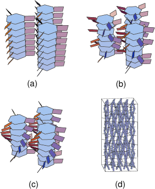
FIG. 1.: Some chiral discotic columnar phases: (a) A uniform orientationally ordered phase in which there is not twist. This twist has been expelled as in the smectic-$A$ phase of chiral molecules, (b) An orientationally disordered or “plastic” columnar phase. The is no long-range orientational order of the molecules, but the hexagonal columnar structure remains intact. (c) A cholesteric-like phase in which molecules rotate in a helical fashion within each column while maintaining phase coherence between columns. (d) The moiré phase in which the columns themselves rotate about the $z$ axis. Rotations occur in discrete jumps about twist grain boundaries. (From Ref. [7])

In this paper, we will introduce a fairly general model for chiral columnar phase that has soliton and moiré phases in addition to phases with expelled twist. To keep the model as simple as possible, we restrict the normal to the disc-like molecules to lie parallel to the columnar axes. We will, therefore, not be able to discuss the tilt-grain-boundary phase or ferroelectric chiral discotics. In a future publication, we will study a variety of phases that can result with this constraint is relaxed. Our model begins with interacting chiral molecules in a discotic columnar phase. Its Hamiltonian has an elastic part associated with distortions of the lattice. It has terms favoring parallel alignment of neighboring molecules and chiral terms favoring both molecular and lattice rotation. It also has crystal-field terms coupling molecular orientation to the columnar lattice and defining a twist penetration depth $\lambda_{\theta}$ analogous to that of smectic systems. If lattice distortions are prohibited, our model is essentially identical to that studied by the Sherbrooke group[9]. We assume that the low-temperature, weak chirality, ground state of our Hamiltonian is the ordered “ferromagnetically” aligned state shown in Fig. 1a, though other large unit-cell states are possible[9]. As chirality is increased, the aligned state can become unstable either to a soliton lattice if the crystal-field coupling is weak or to a moiré phase if it is strong. Our primary aim will be to determine the critical chirality for these two instabilities. Our model, however, has the potential for more complicated phases and very complex phase diagrams. For example, a mixed moiré-soliton phase in which there is molecular twist relative to the lattice between grain boundaries could exist. Or the soliton phase could melt altogether to a “plastic” discotic phase with no orientational long-range order (Fig. 1b). This phase could them become unstable with respect to the formation of a moiré phase.

Though our model is motivated by chiral discotic liquid crystals, it can, with proper interpretation, be applied to aligned chiral polymers such as DNA[10]. Aligned polymers can form a hexagonal lattice perpendicular to the direction of alignment. A polymer like DNA is a tightly wound double helix. This structure makes it unlikely for it to form an orientationally ordered phase analogous to the discotic ground state shown in Fig. 1a. Rather the phases of the molecular helices on neighboring molecules will be random: there will be no long-range order in molecular orientations perpendicular to the direction of polymeric alignment. The ground state will be equivalent to the disordered states shown in Fig. 1b, though each molecule will have an average twist. Thus, there is no analog of the soliton phase in DNA, and the moiré phase is driven by chiral terms favoring lattice rotation rather than molecular rotation.

The outline of this paper is as follows. In Sec. II, we define the model and discuss its continuum limt. In Sec. III we discuss instabilities toward the moiré phase. This analysis differs from that of reference [7] because of the finite twist penetration depth. Our results are, however, almost identical to those of that reference. In Sec. IV, we discuss the soliton phase and arrive at a criterion determining whether the soliton or the moiré phase will form.

II The Model

A The Lattice Model

Columnar forming chiral molecules can come in many forms. We will limit our discussion to molecules such as that shown in Fig. 2 with $C_{3}$ symmetry. This molecule is similar to some that have recently been synthesized[5] and to those spontaneously formed in the experiments of Heiney[8]. Since we are interested principally in the competition between soliton and moiré phases, we will assume that the molecular normal always aligns along the columnar direction. We will, therefore, not be able to discuss the formation of the tilt-grain-boundary phase. We use a mixed continuum-lattice description of the columnar phase. The discotic columns form a two-dimensional hexagonal lattice with lattice parameter $a$. They are labeled by an index ${\bf l}$. Distance parallel to the columns is specified by the continuous coordinate $z$. The orientation of molecules at position $z$ in column ${\bf l}$ is specified by the angle $\theta_{{\bf l}}(z)$. The column coordinates are given by ${\bf X}_{{\bf l}}(z)={\bf R}_{{\bf l}}+{\bf u}({\bf l},z)$ , where ${\bf R}_{{\bf l}}$ is the equilibrium two-dimensional lattice coordinate and ${\bf u}({\bf l},z)$ is displacement from equilibrium that can depend on both $z$ and ${\bf l}$.

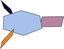
FIG. 2.: Schematic representation of a chiral discotic molecules with $C_{3}$ symmetry. The three vanes coming off the hexagonal core are all tilted in the same direction relative to the normal like the blades of an airplane propeller.

The Hamiltonian for our lattice model can be divided into an elastic part ${\overline{\cal H}}_{\rm el}$, an angle part ${\overline{\cal H}}_{\theta}$, and a chiral part ${\overline{\cal H}}^{*}$. The elastic Hamiltonian is the standard one for a columnar structure. In the harmonic limit, it is

$${\overline{\cal H}}_{\rm el} = {1\over 2}\int dz\sum_{{\bf l},{{\bf l}^{\prime}}}K_{ij}({\bf l},{{\bf l}^{\prime}})u_{i}({\bf l},z)u_{j}({{\bf l}^{\prime}},z)$$ (2)

$$+{1\over 2}\int dz\sum_{{\bf l}}{\overline{\kappa}}[\partial_{z}^{2}{\bf u}({\bf l},z)]^{2}.$$

The first term in this expression, with $K_{ij}({\bf l},{{\bf l}^{\prime}})$ an elastic constant tensor, is the familiar elastic energy of a two-dimensional harmonic lattice of columns. The second term, with ${\overline{\kappa}}$ a bending rigidity, measures the energy of bending the columns. We assume that neighboring molecules want to be parallel in the absence of chirality. Furthermore, there are couplings between lattice distortions and molecular rotation and a preferred orientation of the molecules relative to the lattice. All of these effects are incorporated into the model Hamiltonian

$${\overline{\cal H}}_{\theta} = -{1\over 2}A\int dz\sum_{{\bf l},{{\bf l}^{\prime}}}\cos[3\theta_{{\bf l}}(z)-3\theta_{{{\bf l}^{\prime}}}(z)]$$ (6)

$$-{1\over 2}B\int dz\sum_{{\bf l},{{\bf l}^{\prime}}}\cos[6\theta_{{\bf l}}(z)-6\phi_{{\bf l},{{\bf l}^{\prime}}}(z)]$$

$$-{1\over 2}C\int dz\sum_{{\bf l},{{\bf l}^{\prime}}}\cos[3\theta_{{\bf l}}(z)+3\theta_{{{\bf l}^{\prime}}}(z)-6\phi_{{\bf l},{{\bf l}^{\prime}}}(z)],$$

$$+{1\over 2}{\overline{\kappa}}_{\theta}\sum_{{\bf l}}\int dz[\partial_{z}\theta_{{\bf l}}(z)]^{2}$$

where the sum ${\bf l},{{\bf l}^{\prime}}$ is over nearest neighbor columns in the lattice and

$$\phi_{{\bf l},{{\bf l}^{\prime}}}(z)=\tan^{-1}\left({a_{y}^{{\bf l},{{\bf l}^{\prime}}}+u_{y}({\bf l},z)-u_{y}({{\bf l}^{\prime}},z)\over a_{x}^{{\bf l},{{\bf l}^{\prime}}}+u_{x}({\bf l},z)-u_{x}({{\bf l}^{\prime}},z)}\right)$$ (7)

is the angle the bond between column ${\bf l}$ and ${{\bf l}^{\prime}}$ makes with the $x$-axis at $z$ and ${\bf a}^{{\bf l},{{\bf l}^{\prime}}}$ is the equilibrium lattice vector connecting those columns. The Hamiltonian ${\overline{\cal H}}_{\theta}$ is invariant under $\theta_{{\bf l}}\rightarrow\theta_{{\bf l}}+(2\pi n/3)$ for any interger $n$, as required by the $C_{3}$ molecular symmetry. It is also invariant under rotations of the lattice by $2\pi/6$ and under simultaneous rotations of the molecules and the lattice through arbitrary angles. When lattice distortions are prohibited, ${\overline{\cal H}}_{\theta}$ is very similar to that studied by the Sherbrooke group[9].

Finally chiral interactions along a given column favor molecular rotation, and chiral interactions between molecules in different columns favor lattice rotation. We introduce two chiral terms in our model to describe these effects:

$${\overline{\cal H}}_{\theta}^{*} = -{\overline{\gamma}}_{\theta}\int dz\sum_{{\bf l}}\partial_{z}\theta_{{\bf l}}(z)$$ (8)

$${\overline{\cal H}}_{\phi}^{*} = -{\overline{\gamma}}_{\phi}\sum_{{\bf l},{{\bf l}^{\prime}}}\int dz\partial_{z}\phi_{{\bf l},{{\bf l}^{\prime}}}.$$ (9)

In the ordered phase of discotic systems, the dominant twist comes from ${\overline{\cal H}}_{\theta}^{*}$, and we may assume $\gamma_{\theta}\gg\gamma_{\phi}$. In polymeric systems or in the orientationally disordered phase, $\gamma_{\theta}$ is zero, and any rotation is induced by ${\overline{\cal H}}_{\phi}^{*}$

B The Continuum Limit

When spatial variations are slow on the scale of the lattice spacing, we may expand the lattice Hamiltonian in gradients of lattice displacements ${\bf u}$ and angles $\theta$ and replace the lattice sum by a continuum integral. To this end, we replace ${\bf u}({\bf l},z)$ by ${\bf u}({\bf x})$ and $\theta_{{\bf l}}(z)$ by $\theta({\bf x})$, where ${\bf x}=({\bf x}_{\perp},z)$ with ${\bf x}_{\perp}$ the coordinate perpendicular to $z$, and we set $\int dz\sum_{{\bf l}}\rightarrow a^{-2}\int d^{3}x$. In this limit, the lattice angle $\phi_{{\bf l},{{\bf l}^{\prime}}}(z)$ can be expanded about its equilibrium value of $\phi_{{\bf l},{{\bf l}^{\prime}}}^{0}(z)$ as

$$\delta\phi_{{\bf l},{{\bf l}^{\prime}}}(z) = \phi_{{\bf l},{{\bf l}^{\prime}}}(z)-\phi_{{\bf l},{{\bf l}^{\prime}}}^{0}(z)$$ (10)

$$= a^{-2}[a_{x}^{{\bf l},{{\bf l}^{\prime}}}a_{i}^{{\bf l},{{\bf l}^{\prime}}}\partial_{i}u_{y}({\bf x})-a_{y}^{{\bf l},{{\bf l}^{\prime}}}a_{i}^{{\bf l},{{\bf l}^{\prime}}}\partial_{i}u_{x}({\bf x})].$$ (11)

The Hamiltonian ${\overline{\cal H}}_{\theta}$ does not depend on the equilibrium angle $\phi_{{\bf l},{{\bf l}^{\prime}}}^{0}$ because the latter is an integral multiple of $2\pi/6$. The average over nearest neighbor lattice sites of $\delta\phi_{{\bf l},{{\bf l}^{\prime}}}(z)$ is the hexatic angle $\phi_{6}({\bf x})$:

$$\phi_{6}({\bf x})=\frac{1}{2}\epsilon_{ij}\partial_{i}u_{j}={1\over 6}\sum_{{{\bf l}^{\prime}}}\delta\phi_{{\bf l},{{\bf l}^{\prime}}}(z),$$ (12)

where $\epsilon_{ij}$ is the anti-symmetric two-dimensional tensor with $i$ and $j$ running over $x$ and $y$. In addition,

$$\sum_{{{\bf l}^{\prime}}}[\delta\phi_{{\bf l}{{\bf l}^{\prime}}}^{2}(z)]=6\phi_{6}^{2}+3u_{ij}u_{ij}-\frac{3}{4}u_{ii}^{2},$$ (13)

where $u_{ij}=(\partial_{i}u_{j}+\partial_{j}u_{i})/2$ is the symmetrized strain. With this information, we can express the continuum-limit Hamiltonian as a sum of terms: ${\cal H}={\cal H}_{\rm el}+{\cal H}_{\theta}+{\cal H}_{g}+{\cal H}^{*}$. The elastic Hamiltonian

$${\cal H}_{\rm el}=\frac{1}{2}\int d^{3}x[\lambda u_{ii}^{2}+2\mu u_{ij}u_{ij}+K(\partial_{z}^{2}{\bf u})^{2}],$$ (14)

is the standard continuum elastic Hamiltonian for a hexagonal columnar system. Here $K=\kappa/v_{0}$, where $v_{0}=\sqrt{3}a^{2}/4$ is the area of an hexagonal unit cell, and the Lamé coefficients $\lambda$ and $\mu$ are determined by the continuum limit of $K_{ij}({\bf l},{{\bf l}^{\prime}})$ and by the the parameters $B$ and $C$ in ${\overline{\cal H}}_{\theta}$ through the second order expansion in $\delta\phi_{{\bf l},{{\bf l}^{\prime}}}$. The angle Hamiltonian is simply that of an anisotropic $xy$ model:

$${\cal H}_{\theta}=\frac{1}{2}\int d^{3}x[K_{\theta}^{\perp}(\nabla_{\perp}\theta)^{2}+K_{\theta}^{||}(\partial_{z}\theta)^{2}],$$ (15)

where $K_{\theta}^{||}={\overline{\kappa}}_{\theta}/v_{0}$, $K_{\theta}^{\perp}=9(A+C)/2$, and $\nabla_{\perp}=(\partial_{x},\partial_{y},0)$. The coupling term ${\cal H}_{g}$ is in the small $\theta-\phi_{6}$ limit is

$${\cal H}_{g}={1\over 2}g\int d^{3}x(\theta-\phi_{6})^{2}$$ (16)

where $g=108(B+C)/a^{2}$ and where the final form is valid in the small $\theta$ limit. Finally, the chiral energy becomes

$${\cal H}^{*}=-\gamma_{\theta}\int d^{3}x\partial_{z}\theta-\gamma_{\phi}\int d^{3}x\partial_{z}\phi_{6},$$ (17)

where $\gamma_{\theta}={\overline{\gamma}}_{\theta}/v_{0}$ and $\gamma_{\phi}={\overline{\gamma}}_{\phi}/v_{0}$.

The continuum Hamiltonian has a structure imposed by rotational invariance: the coupling term $\frac{1}{2}g(\theta-\frac{1}{2}\epsilon_{ij}\partial_{i}u_{j})^{2}$ is invariant under simultaneous rotations of the lattice and molecular orientations. It is the analog for columnar systems of the invariant coupling[11] $(\delta{\bf n}+\nabla u)^{2}$ of smectic-$A$ liquid crystals, where $\delta{\bf n}$ is the deviation of the Frank director form its equilibrium orientation. The columnar phase, like the smectic-$A$ phase tends to expel molecular twist. In the ground state, molecules align along preferred crystal axes with $\theta=0$. A twist in $\theta$ relative to the lattice at $z=0$ will decay to zero in twist penetration depths

$$\lambda_{\theta}^{||}=\sqrt{K_{\theta}^{||}/g},\qquad\lambda_{\theta}^{\perp}=\sqrt{K_{\theta}^{\perp}/g},$$ (18)

which tend to zero in this strong coupling, $g\rightarrow\infty$ limit. Another important length is

$$\lambda=\sqrt{K/\mu}$$ (19)

giving the length scale over which bend deformations heal.

Two limits of the continuum Hamiltonian deserve special attention. The first is that in which there is no long-range orientational order. In this limit, $\theta$ looses its meaning, and only terms involving ${\bf u}$ remain. The Hamiltonian becomes ${\cal H}_{\rm el}+{\cal H}_{\phi}^{*}$ with, in particular, $g=0$. This is the limit studied in [7]. The second is the strong-coupling $g\rightarrow\infty$ limit in which $\theta$ and $\phi_{6}$ are forced to be equal. This leads to ${\cal H}^{*}=-(\gamma_{\theta}+\gamma_{\phi})\int d^{3}x\partial_{z}\phi_{6}$ and ${\cal H}_{\theta}=\frac{1}{8}\int d^{3}x[K_{\theta}^{\perp}(\nabla_{\perp}\epsilon_{ij}\partial_{i}u_{j})^{2}+K_{\theta}^{||}(\partial_{z}\epsilon_{ij}\partial_{i}u_{j})^{2}]$. Thus, except for a $(\partial^{2}u)^{2}$ correction, the form of the Hamiltonian with $g=\infty$ is identical to that for $g=0$. We should expect, therefore, that the critical values of chiral couplings leading to the moiré phase will have similar forms but differ in magnitude in the two limits and that there will be a smooth, non-singular interpolation between these limits as a function of $g$.

III The Soliton Phase

If the coupling $g$ between molecular and lattice rotations is weak, molecules will be able to rotate relative to the fixed lattice. We can describe this situation by a Hamiltonian depending only on $\theta$ and not on ${\bf u}$: ${\cal H}={\cal H}_{\theta}+{\cal H}_{g}+{\cal H}_{\theta}^{*}$, where

$${\cal H}_{g}=-\frac{1}{36}g\int d^{3}x\cos 6\theta.$$ (20)

This Hamiltonian is a chiral Sine-Gordon model that is equivalent to the continuum limit of the Frenkel-Kontorowa model[12] and that describes a cholesteric liquid crystal in an external field. The chiral term ${\cal H}_{\theta}^{*}$ favors twist that the angle elastic term ${\cal H}_{\theta}$ oposes. Twist sets in when the coupling $g$ exceeds the critical value necessary to nucleate a single soliton, which produces a rotation of $\theta$ through an angle of $\pi/3$ from one end of the sample to another. The energy per unit area of a single soliton is

$$\sigma={2\over 9}\sqrt{K_{\theta}^{||}g}={2\over 9}g\lambda_{\theta}^{||}.$$ (21)

The chiral energy gain arising from a single soliton is ${\cal H}_{\theta}^{*}=-A(\pi/3)\gamma_{\theta}$, where $A$ is the area. Thus the total energy per unit area of a single soliton is

$$f_{s}=[\sigma-(\pi\gamma_{\theta}/3)].$$ (22)

The critical chiral coupling constant is, therefore,

$$\gamma_{\theta}^{s}={2\over 3\pi}\sqrt{gK_{\theta}^{||}}.$$ (23)

For $\gamma_{\theta}>\gamma_{\theta}^{s}$, there will be a soliton lattice in $\theta$ with a lattice spacing that decreases with increasing $\gamma_{\theta}$. This is a helical state with a pitch equal to the soliton lattice spacing.

IV The Moiré Phase

The moiré phase consists of a periodic array of twist grain boundaries perpendicular to the columnar axis across which the orientation of the hexagonal lattice rotates in discrete jumps. The twist grain boundary is a honeycomb lattice of screw dislocations. This phase forms when the energy cost of creating a low-angle grain boundary is just counterbalanced by the twist energy gain arising from ${\cal H}^{*}$. Let $l_{b}$ be the distance between grain boundaries and $l_{d}$ be the length of the side of the hexagonal unit cell of the honeycomb dislocation lattice (see Fig. 3). The total length of screw dislocations in a lattice of $N$ cells is $L=3Nl_{d}$. The total area of this lattice is $A=3Nl_{d}^{2}/2\sqrt{3}$. In the limit of large lattice spacing (i.e., large $l_{b}$ and $l_{d}$), interactions between dislocations can be neglected, and the energy per unit volume of an array of low-angle grain boundaries is $f_{GB}=\epsilon_{d}L/(Al_{b})=2\epsilon_{d}/(l_{d}\sqrt{3}l_{b})$, where $\epsilon_{d}$ is the energy per unit length of a dislocation. Far from the boundary, $\theta=\phi_{6}$, and both $\theta$ and $\phi_{6}$ undergo the same jump $\Delta\theta$ across the boundary. This jump was calculated in Ref. [7]. It is $b/l_{d}\sqrt{3}$ where $b=d$ is the magnitude of the Burgers vector. The chiral energy of an array of grain $N$ boundaries is thus

$${\cal H}^{*}=NA{\gamma b\over l_{d}\sqrt{3}}=V{\gamma b\over\sqrt{3}l_{b}l_{d}},$$ (24)

where $\gamma=\gamma_{\theta}+\gamma_{\phi}$ and $V=NAl_{b}$ is the volume. Thus, the energy per unit volume of the moiré phase when dislocations interactions are ignored is

$$f_{m}={1\over\sqrt{3}l_{d}l_{b}}(2\epsilon_{d}-\gamma b).$$ (25)

This energy becomes negative, and the moiré state becomes energetically preferable to the ordered phase when $\gamma>\gamma^{m}$, where

$$\gamma^{m}=2\epsilon_{d}/b.$$ (26)

This result does not depend on the particular type of dislocation lattice formed in the grain boundary. For example, if the grain boundary consists of identical orthogonal grids of dislocations with separation $l_{d}$ between dislocations then $L=2l_{d}$, $A=l_{d}^{2}$, and $\Delta\theta=b/l_{d}$ so that $f_{m}=(2\epsilon_{d}-\gamma b)/(l_{d}l_{b})$, again producing $\gamma^{m}=2\epsilon_{d}/b$.

FIG. 3.: Honeycomb lattice of screw dislocations that comprise twist grain boundaries in the moiré phase

The ordered phase becomes unstable with respect to the formation of the moiré phase when $\gamma$ exceeds $\gamma_{m}$. Our task, therefore, is to calculate the energy per unit length of a screw dislocation $\epsilon_{d}$. We follow closely the procedure of Ref. [13] appropriately generalized to include $\theta$ as an independent variable. We introduce $w_{\gamma i}$, which is equal to $\partial_{\gamma}u_{i}$ away from defects, where $i=1,2$ and $\gamma=x,y,z$. We also introduce the dislocation density,

$$\alpha_{\gamma i}({\bf x})=\sum_{n}\int ds\,t_{n,\gamma}(s)b_{n,i}\delta^{(3)}({\bf R}_{n}(s)-{\bf x}),$$ (27)

where ${\bf R}_{n}(s)$ is the position vector of dislocation $n$ with Burgers vector ${\bf b}_{n}$ as a function of its arclength $s$ and ${\bf t}_{n}(s)=d{\bf R}_{n}(s)/ds$ is its unit tangent vector. The condition $\oint_{\partial\Gamma}du_{i}=b_{i}$ that the integral of the changes in ${\bf u}$ around a contour $\partial\Gamma$ enclosing a dislocation with Burgers vector ${\bf b}$ be equal to ${\bf b}$ then implies the constraint,

$$\epsilon_{\mu\nu\gamma}\partial_{\nu}w_{\gamma i}=\alpha_{\mu i}({\bf x}),$$ (28)

on $w_{\gamma i}$. To find the elastic energy associated with dislocations, we need to minimize the energy ${\cal H}={\cal H}_{\rm el}+{\cal H}_{\theta}$ subject to this constraint. Minimizing ${\cal H}$ with respect to variations in $\theta$ and ${\bf u}$, we obtain

$${\delta{\cal H}\over\delta\theta} = -K^{\perp}_{\theta}\nabla^{2}_{\perp}\theta-K^{||}_{\theta}\nabla^{2}_{||}\theta+g(\theta-\frac{1}{2}\epsilon_{ij}w_{ij})=0,$$ (29)

$${\delta{\cal H}\over\delta u_{j}} = -\mu(\partial_{i}w_{ij}+\partial_{i}w_{ji})-\lambda\partial_{j}w_{ii}+K\partial_{z}^{3}w_{zj}$$ (31)

$$+{g\over 2}(\epsilon_{ij}\partial_{i}\theta-{1\over 2}\epsilon_{ij}\epsilon_{ij^{\prime}}\partial_{i^{\prime}}w_{i^{\prime}j^{\prime}})=0.$$

After Fourier transforming, we can solve Eqs. (29) and (28) for $\theta$ and $w_{\gamma,i}$:

$$\theta = {g\epsilon_{ij}w_{ij}\over 2(K_{\theta}^{||}q_{||}^{2}+K_{\theta}^{\perp}q_{\perp}^{2}+g)}$$ (32)

$$w_{\gamma i} = {-i\epsilon_{\gamma\mu\nu}q_{\mu}\alpha_{\nu i}({\bf q})\over q^{2}}+iq_{\gamma}\psi_{i}({\bf q})$$ (33)

where $\psi_{i}=i(q_{i}\sigma-\epsilon_{ij}q_{j}\pi)/q_{\perp}^{2}$ defines the longitudinal part, which is obtained by solving Eq. (31). Substituting Eq. (32) into Eq. (31) and using $q_{i}\psi_{i}=i\sigma$ and $\epsilon_{li}q_{l}\psi_{l}=i\pi$, we obtain

$$i\sigma = {1\over(2\mu+\lambda)q_{\perp}^{2}+Kq_{z}^{4}}\left[{\lambda\epsilon_{lm}q_{\perp}^{2}q_{m}\alpha_{zl}({\bf q})\over q^{2}}\right.$$ (35)

$$\left.-{2\mu-Kq_{z}^{2}\over q^{2}}\epsilon_{lm}q_{l}q_{j}q_{z}\alpha_{mj}\right],$$

$$i\pi = {1\over(\beta(q)+\mu)q_{\perp}^{2}+Kq_{z}^{4}}$$ (38)

$$\times\left[-\beta({\bf q})q_{\perp}^{2}(q_{\perp}^{2}q_{n}\alpha_{zn}({\bf q})+q_{\perp}^{2}q_{z}\alpha_{nn}({\bf q})\right.$$

$$+\left.{\mu+Kq_{z}^{2}\over q^{2}}q_{z}q_{l}q_{i}\epsilon_{lj}\epsilon_{im}\alpha_{mj}-{\mu\over q^{2}}q_{l}q_{i}q_{\rho}\epsilon_{lj}\epsilon_{j\rho\nu}\alpha_{\nu i}(q)\right]$$

where

$$\beta({\bf q})={1\over 4}{g(K_{\theta}^{||}q_{||}^{2}+K_{\theta}^{\perp}q_{\perp}^{2})\over g+K_{\theta}^{||}q_{||}^{2}+K_{\theta}^{\perp}q_{\perp}^{2}}.$$ (39)

For a single screw dislocation aligned along the $x$-axis. $\alpha_{\nu i}({\bf q})=2\pi b\delta_{\nu x}\delta_{ix}\delta(q_{x})$. Using Eqs. (33, (35), and (38), we obtain

$$w_{yx}(q) = {-iq_{z}\alpha_{xx}(q)\over q^{2}}{Kq^{2}q_{z}^{2}\over{\overline{\mu}}({\bf q})q_{y}^{2}+Kq_{z}^{4}},$$ (40)

$$w_{zx}(q) = {iq_{y}\alpha_{xx}(q)\over q^{2}}{{\overline{\mu}}({\bf q})q^{2}\over{\overline{\mu}}({\bf q})q_{y}^{2}+Kq_{z}^{4}},$$ (41)

where

$${\overline{\mu}}({\bf q})=\mu+\beta({\bf q}).$$ (42)

Then, using Eq. (41) in ${\cal H}$, we obtain the energy per unit length of a dislocation,

$${\epsilon_{d}}={1\over 2}Kb^{2}\int{dq_{y}dq_{z}\over(2\pi)^{2}}{q_{z}^{2}{\overline{\mu}}({\bf q})\over{\overline{\mu}}({\bf q})q_{y}^{2}+Kq_{z}^{4}},$$ (43)

where the integrals over $q_{y}$ and $q_{z}$ have respective upper cutoffs of the inverse correlation lengths, $\xi_{\perp}^{-1}$ and $\xi_{||}^{-1}$. This expression is identical to that obtained in Ref. [7] with ${\overline{\mu}}({\bf q})$ replacing $\mu$.

To evaluate ${\epsilon_{d}}$, it is convenient to express the integral in a unitless form:

$${\epsilon_{d}}=\epsilon_{0}\int_{0}^{1}dy\int_{0}^{1}dz{z^{2}(1+f)\over y^{2}(1+f)+\delta^{4}z^{4}},$$ (44)

where

$$\epsilon_{0}={Kb^{2}\over 8\pi^{2}}{\xi_{\perp}\over\xi_{||}^{3}}$$ (45)

and

$$f={\beta_{||}^{2}z^{2}+\beta_{\perp}^{2}y^{2}\over 1+\alpha_{||}^{2}z^{2}+\alpha_{\perp}^{2}y^{2}}.$$ (46)

In the expressions for ${\epsilon_{d}}$ and $f$, we have introduced unitless ratios, all of which are Ginzburg parameters measuring the ratio of a penetration depth to a coherence length. The parameter

$$\delta={\sqrt{\lambda\xi_{\perp}}\over\xi_{||}}$$ (47)

was introduced in Ref. [7]. The parameters

$$\alpha_{||}={\lambda_{\theta}^{||}\over\xi_{||}}\qquad\alpha_{\perp}={\lambda_{\theta}^{\perp}\over\xi_{\perp}}$$ (48)

and

$$\beta_{||} = {1\over 2\xi_{||}}\sqrt{K_{\theta}^{||}\over\mu}={\lambda\over 2\xi_{||}}\sqrt{K_{\theta}^{||}\over K},$$ (49)

$$\beta_{\perp} = {1\over 2\xi_{\perp}}\sqrt{K_{\theta}^{\perp}\over\mu}={\lambda\over 2\xi_{\perp}}\sqrt{K_{\theta}^{\perp}\over K}$$ (50)

are Ginzburg parameters for twist penetration. Note that $\beta_{\perp}$ and $\beta_{||}$ are independent of $g$.

Analytic evaluation of ${\epsilon_{d}}$ is difficult except for $g=0$. We will content ourselves with the $\delta\rightarrow 0$ and $\delta\rightarrow\infty$ limits for $g$ small and for $g-\infty$. Since $d{\epsilon_{d}}/dg$ is positive, ${\epsilon_{d}}$ will increase monotonically from the its value at $g=0$ to its value at $g=\infty$. As $g\rightarrow 0$, we find

1. $g\rightarrow 0$, $\delta=0$

   $${\epsilon_{d}} = {\pi\over 2}\epsilon_{0}\delta^{-2}\left(1+{1\over 8}{g\over\mu}\right)$$ (51)

   $$= {1\over 16\pi}{K^{1/2}\mu^{1/2}b^{2}\over\xi_{||}}\left(1+{g\over 8\mu}\right),$$ (52)

   and

2. $g\rightarrow 0$, $\delta=\infty$

   $$\epsilon_{d} = {\pi\over\sqrt{2}}\epsilon_{0}\delta^{-3}\left(1+{3\over 16}{g\over\mu}\right)$$ (53)

   $$= {1\over 8\sqrt{2}\pi}{\mu^{3/4}K^{1/4}b^{2}\over\sqrt{\xi_{\perp}}}\left(1+{3\over 16}{g\over\mu}\right).$$ (54)

For $g=\infty$, we find

1. $g=\infty$, $\delta\rightarrow 0$

   $${\epsilon_{d}} = {\pi\over 2}\epsilon_{0}\delta^{-2}$$ (56)

   $$\times\left[{1\over 2}\sqrt{1+\beta_{||}^{2}}+{1\over 2\beta_{||}}\ln(\beta_{||}+\sqrt{1+\beta_{||}^{2}})\right]$$

2. $g=\infty$, $\delta=\infty$

   $${\epsilon_{d}}={\pi\over\sqrt{2}}\epsilon_{0}\delta^{-3}{1\over 2}\int_{0}^{1}dyy^{-1/2}(1+\beta_{\perp}^{2}y^{2})^{3/4}$$ (57)

These results reduce to those of reference [7] (when a missing factor of $1/4$ is added). ${\epsilon_{d}}$ increases smoothly and monotonically with $g$. Its value at $g=\infty$ is finite and depends on the Ginzburg parameters $\beta_{\perp}$ and $\beta_{||}$. When $\beta_{||}$ and $\beta_{\perp}$ are both zero, $f=0$, and ${\epsilon_{d}}(g)={\epsilon_{d}}(g=0)$. When these quantities are much greater than unit, ${\epsilon_{d}}(g=\infty)\gg{\epsilon_{d}}(g=0)$:

$${{\epsilon_{d}}(g=\infty,\delta=0)\over{\epsilon_{d}}(g=0,\delta=0)} \rightarrow{1\over 2}\beta_{||},\qquad\beta_{||}\gg 1$$ (58)

$${{\epsilon_{d}}(g=\infty,\delta=\infty)\over{\epsilon_{d}}(g=0,\delta=\infty)} \rightarrow{1\over 4}\beta_{\perp}^{3/2},\qquad\beta_{\perp}\gg 1.$$ (59)

Thus, large $g$ and large angle elastic constants $K_{\theta}^{||}$ and $K_{\theta}^{\perp}$ lead to large values of ${\epsilon_{d}}$ and suppress the formation of the moiré phase.

V Discussion and Review

In this paper, we have developed a model for chiral discotic columnar liquid crystals, and we have investigated its instability toward the formation of two types of structurally chiral phases: the soliton phase and the moiré phase. Chirality in our model, which restricts the average molecular normal to be along the columnar axis, gives rise to two kinds of chiral interactions, one tending to rotate molecules within a column and the other tending to rotate the columns themselves. These two interactions are characterized by respective coupling strengths $\gamma_{\theta}$ and $\gamma_{\phi}$. There is an energy cost associated with rotation of molecules relative to the lattice characterized by a coupling constant $g$. When $g$ is small, rotation of molecules within columns with a fixed lattice structure is possible. This is the soliton phase that develops for molecular chiral coupling constant $\gamma_{\theta}$ greater than a critical value $\gamma_{\theta}^{s}\sim\sqrt{g}$. When $g$ is larger formation of the moiré phase is favored for $\gamma_{\theta}+\gamma_{\phi}>\gamma^{m}$ where $\gamma^{m}$ is a smooth function of $g$ that is finite in the $g\rightarrow\infty$ limit.

We have focussed on the instabilities toward two possible structurally chiral phases. A full phase diagram for the model and indeed for real chiral discotic systems can be quite complex with mixed soliton-moiré phases. Additional phases can occur if the constraint that the molecular normal (the Frank director) be parallel to the columnar axis be relaxed. In particular, tilt-grain-boundary phases and smectic-$C^{*}$-like phase in which the director tilts relative to the columnar axis and rotates in a helical fashion along that axis can occur. These more complex phase are currently being investigated.

We are extremely grateful for many conversations with and continuous support from Randall Kamien. We also acknowledge useful converstions with Tim Swager. This work primarily by the MRSEC Program of the National Science Foundation under Award Number DMR96-32598.

REFERENCES

• [1] P.G. de Gennes and J. Prost, The Physics of Liquid Crystals, 2nd edn. (Clarendon Press, Oxford, 1993).
• [2] Jacques Malthête, C. Destrade, Nguyen Tinh, and J. Jacques, Molec. Cryst. Liq. Cryst. 66, 115 (1981); Jacques Malthête, Jean Jacques, Nguyen Tinh, and Christian Destrade, Nature 298, 46 (1982)
• [3] Harald Bock and Wolfgang Helfrich, Liquid Crystals 18, 387 and 707 (1995).
• [4] Günther Scherowskyu and Sin Hus Chen, Liquid Crystals 17, 803 (1994).
• [5] Hanxing Zheng and Timothy M. Swager, private communication
• [6] S.R. Renn and T.C. Lubensky, Phys. Rev. A 38, 2132 (1988); 51, 4392 (1990).
• [7] Randall D. Kamien and David R. Nelson, Phys. Rev. Lett. 74, 2499 (1995); Phys. Rev. E 53, 650 (1996).
• [8] E. Fontes, P.A. Heiney, and W.H. de Jeu, Phys. Rev. Lett. 61, 1202 (1988); P.A. Heiney, E. Fontes, W.H. de Jeu, A. Reira, P. Carroll, and a.B. Smith III, J. Phys. (Paris) 50 461 (1989).
• [9] M.L. Plumer, A. Caillé, and O. Heinonen, Phys. Rev. B 47 8479 (1993); M. Hébert, A. Caille, and A. Bel Moufid, Phys. Rev. B 48, 3074 (1993); M. Hébert and A. Caillé, Phys. Rev. E 53, 1714 (1996).
• [10] F. Livolant, Physica A 176, 117 (1981); R.L. Hill, T.E. Strzelecka, D.H. Van Winkle, and M.W. Davidson, Physics A 176, 87 (1991); A. Le Forestier and F. Livolant, Biophys. J. 65, 56 (1994); R. Podgornik, et. al., Proc. Nat. Acad. Sci. 93, 4261 (1996).
• [11] See for example, P.M. Chaikin and T.C. Lubensky, Principles of Condensed Matter Physics (Cambridge University Press, Cambridge, 1995), Sec. 6.3.
• [12] Y.I. Frenkel and T. Kontorowa, Zh. Eksp. Teor. Fiz. 8, 1340 (1938); Reference [11], Sec. 10.3.
• [13] A.M. Kosevic, Usp. Fiz. Nauk 84, 579 (1964) [Sov. Phys. Usp. 7, 837 (1965)];