Discrete Folding

Abstract

Models of folding of a triangular lattice embedded in a discrete space are studied as simple models of the crumpling transition of fixed-connectivity membranes. Both the case of planar folding and three-dimensional folding on a face-centered-cubic lattice are treated. The 3d-folding problem corresponds to a 96-vertex model and exhibits a first-order folding transition from a crumpled phase to a completely flat phase as the bending rigidity increases.

1 Introduction

The statistical mechanics of polymers, essentially one-dimensional objects, has proven to be a rich and fascinating field.[1, 2] The success of physical methods applied to polymers arises from universality — many of the large-length-scale properties of polymers are independent of microscopic details such as the chemical identity of the monomers. The generalization of polymer statistical mechanics to membranes, two-dimensional surfaces fluctuating in some embedding space, has proven to be even richer and is still under active development. In contrast to polymers there are different universality classes of membranes distinguished by their long-range order. These classes are the analogues of the well-known crystalline, hexatic and fluid phases of strictly two-dimensional systems.[3, 4] This diversity arises from the richer geometry of surfaces as compared to lines and the resultant enlarged space of possible symmetries.

The closest membrane analogue to a polymer is a $2D$ fishnet-like mesh of monomers (or vertices) with fixed connectivity. The bonds (links) are assumed to be unbreakable. The vertices themselves live in ${\bf R}^{d}$, with a physical membrane corresponding to the case $d=3$. Such a membrane is called a crystalline or polymerized membrane by virtue of its intrinsic crystalline order. In this talk we will deal only with phantom (non-self-avoiding) membranes. In general the Hamiltonian for a polymerized membrane will have both in-plane elastic (strain) contributions and out-of-plane bending contributions, since it can both support shear and fluctuate in the embedding space. In Monge gauge the most general effective continuum Hamiltonian at long wavelength takes the form

$${\cal H}(h,{\bf u})=\frac{\kappa}{2}\int d^{2}\sigma\,{(\nabla^{2}h)}^{2}+\frac{1}{2}\int d^{2}\sigma(2\mu\,u_{\alpha\beta}^{2}+\lambda\,u_{\gamma\gamma}^{2}),$$ (1)

where $h$ is the height above a reference plane with intrinsic coordinates $(\sigma_{1},\sigma_{2})$, ${\bf u}$ are the phonon modes, $u_{\alpha\beta}$ is the strain tensor, $\kappa$ is the bending rigidity and $\mu$ and $\lambda$ are the bare Lamé coefficients. The strain tensor $u_{\alpha\beta}$ measures the difference between the induced metric and a flat reference metric determined by the equilibrium configuration of the membrane at rest.

The distinctive physics of polymerized membranes arises from an unavoidable nonlinear coupling between the in-plane strain modes and the out-of-plane height fluctuations. Integrating out the quadratic phonon fluctuations by linearizing the strain tensor one finds an effective long-range interaction between Gaussian curvature excitations which tends to stiffen the surface on long length scales.[5, 3] In other words, the effect of undulations on small length scales is to increase the bending rigidity on longer length scales. This effect is easily demonstrated — an ordinary piece of paper becomes much stiffer with respect to bending deformations after it is crumpled and then opened up. More technically, one finds that the bending rigidity at sufficiently long wavelengths is momentum dependent $\kappa(q)\sim q^{-\eta}$, with $\eta$ positive. This scaling behaviour leads to a stable flat phase for polymerized membranes,[5, 3] with remarkable properties controlled by a infrared stable fixed point.[6, 7, 8] For small bending rigidity (high-temperature), on the other hand, polymerized membranes are crumpled.[9] At some critical bending rigidity (or equivalently critical temperature) there should, therefore, be a crumpling transition from a flat to a crumpled phase.

The flat phase of polymerized membranes is characterized by long-range orientational order in the surface normals. Since long-range order is unusual in $2D$ systems it is worthwhile to explore as many avenues as possible to understand its exact nature and origin. Aronovitz and Lubensky [6] analyzed the flat phase of $D$-dimensional elastic solids embedded in ${\bf R}^{d}$, and subject to bending energy, using an $\epsilon$ expansion about the upper critical (manifold) dimension $D_{uc}=4$, with fixed codimension $d_{c}=d-D$. They determined the renormalization group flows in the space of dimensionless couplings $\hat{\mu}=\mu l^{\epsilon}/\kappa^{2}$ and $\hat{\lambda}=\lambda l^{\epsilon}/\kappa^{2}$, where $l$ is the renormalization length scale. They discovered a globally attractive infrared fixed point describing a flat phase and determined the scaling dimension $\eta$ and the corresponding exponent $\eta_{u}$ ($\mu\sim\lambda\sim q^{\eta_{u}}$) for the infinite renormalization of the Lamé coefficients.

A revealing extreme limit of polymerized membranes was studied by David and Guitter.[10] This is the limit of infinite Lamé coefficients in the Hamiltonian (1). Since the elastic term scales like $q^{2}$, in momentum space, as compared to $q^{4}$ for the bending term, this limit may be regarded as a means of determining the dominant infrared behaviour of (1). In this “stretchless” limit the strain tensor $u_{\alpha\beta}$ must vanish and the model is constrained, very much in analogy to a non-linear sigma model. The $\beta$-function for the suitably rescaled inverse bending rigidity $\alpha=d/\kappa$ may then be computed in the large-$d$ limit, yielding

$$\beta(\alpha)=q\frac{\partial\alpha}{\partial q}=\frac{2}{d}\ \alpha-(\frac{1}{4\pi}+\frac{{\rm const}}{d})\ \alpha^{2}.$$ (2)

For $d=\infty$ there is no stable fixed point [11] and the membrane is always crumpled. Eq. 2 reveals, to next order in $1/d$, an ultraviolet stable fixed point at $\alpha=8\pi/d$, corresponding to a continuous crumpling transition. The critical exponents associated with the “flat” fixed point, discussed above, may also be determined in the large-$d$ expansion.[7]

2 Folding

A natural lattice formulation of the infinite-elastic-constant limit is the statistical mechanics of folding of a regular triangular lattice. A folding in ${\bf R}^{d}$ of the regular triangular lattice is a mapping which assigns to each vertex $v$ of the triangular lattice a position ${\bf X}_{v}$ in the $d$-dimensional embedding space ${\bf R}^{d}$, with the “metric” constraint that the Euclidean distance $|{\bf X}_{v_{2}}-{\bf X}_{v_{1}}|$ in ${\bf R}^{d}$ between nearest neighbours $v_{1}$ and $v_{2}$ on the lattice is always unity. Under such a mapping, each elementary triangle of the lattice is mapped onto an equilateral triangle in ${\bf R}^{d}$. In general, two adjacent triangles form some angle in ${\bf R}^{d}$, i.e. links serve as hinges between triangles and may be (partially) folded.

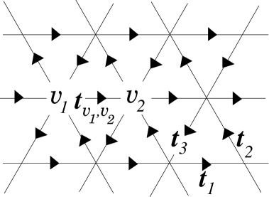
Figure 1: The oriented triangular lattice: triangles pointing up (resp. down) are oriented counterclockwise (resp. clockwise). The three tangent vectors ${\bf t}_{i}$, $i=1,2,3$, have a vanishing sum in the embedding space.

Folding is best described in terms of tangent vectors, which are link variables defined as follows: we first orient the links of the lattice as in Fig.1, with triangles pointing up (resp. down) oriented counterclockwise (resp. clockwise), and define the tangent vector between two neighbours $v_{1}$ and $v_{2}$ as the vector ${\bf t}_{v_{1},v_{2}}={\bf X}_{v_{2}}-{\bf X}_{v_{1}}$ if the arrow points from $v_{1}$ to $v_{2}$. The metric constraint states that all tangent vectors have unit length. With our choice of orientation, moreover, the three tangent vectors ${\bf t}_{i}$, $i=1,2,3$, around each face of the lattice must have vanishing sum. This is the basic folding rule:

$${\bf t}_{1}+{\bf t}_{2}+{\bf t}_{3}={\bf 0}.$$ (3)

Up to a global translation in ${\bf R}^{d}$, a folding is therefore a configuration of unit tangent vectors defined on the links of the lattice, obeying the folding rule (3) around each triangle.

Viewed in terms of normals membrane models resemble non-linear sigma models. In the lattice version the correspondence is with Heisenberg spin models. There is one key difference — apparent in both the continuum and lattice models. Normal vectors are not arbitrary unit vectors in the embedding space — they are constrained to be normal to the underlying $2D$ manifold. This means they are actually Grassmannian sigma models in the continuum [12] and constrained Heisenberg models on the lattice. These constraints play a crucial role in stabilizing an ordered phase.

3 Planar Folding

The two-dimensional or planar ($d=2$) folding problem of the triangular lattice was first introduced and studied numerically by Kantor and Jarić.[13] It is clear that the only remnant of the normal vector degree of freedom is a $Z_{2}$ spin corresponding to orientation (up or down). As an Ising spin system the planar folding model is constrained (as noted above) and is described by an 11-vertex model. In folding terms these 11 vertices describe the distinct folded states of a single hexagon of the original triangular lattice. In terms of the total magnetization $M$ the analogue of the crumpling transition for this model would be a spin-ordering transition from an unmagnetized phase ($M=0$) to a magnetized phase ($M\neq 0$). Analytic progress on planar folding was made subsequently.[14] For planar folding it is easy to check that, up to a global rotation in the embedding plane, all the link variables are forced to take their values among a fixed set of three unit vectors with vanishing sum. This permits a reformulation of the pure planar folding problem (with no bending rigidity) as that of the 3–colouring of the links of the triangular lattice: calling the three fixed vectors blue, white and red, the folding rule (3) translates into the constraint that the three colours around each triangle be distinct. This 3–colouring problem was solved by Baxter [15] with Bethe Ansatz and transfer matrix techniques. His result for the thermodynamic partition function measures the number of distinct folded configurations $Z_{2d}\propto q_{2d}^{N_{\Delta}}$ for a lattice with $N_{\Delta}$ triangles, in the limit of large $N_{\Delta}$. This gives the folding entropy per triangle $s_{2d}=\log(q_{2d})$, with [14]

$${q_{2d}=\frac{\sqrt{3}}{2\pi}\Gamma(1/3)^{3/2}=1.20872...}$$ (4)

The $2d$ folding problem has also been studied in the presence of bending rigidity, which associates an energy to each folded link, and with a magnetic field coupled to the sum of the normal vectors to the lattice.[16] The model was found to undergo a first order folding transition. At zero rigidity and zero magnetic field, the lattice is in an entropic folded phase ($M=0$). At large enough rigidity and/or magnetic field, the lattice becomes totally unfolded ($M=\pm 1$).

Figure 2: The phase diagram for planar folding in the (K,h) plane, where K is the discrete bending rigidity and h is an external magnetic field. Three first order lines ${\rm h}={\rm h}_{\rm c}({\rm K}),-{\rm h}_{\rm c}({\rm K})\;({\rm K}<{\rm K}_{\rm c})$ and ${\rm h}=0\;({\rm K}>{\rm K}_{\rm c})$ separate the three phases ${\rm M}=0,\pm 1$ and meet at the triple point $({\rm K}_{\rm c},0)$.

The phase diagram is shown in Fig. 2.

4 Three-Dimensional Folding

The existence of a unfolded (magnetized) phase and a first-order folding transition is fascinating, but one would like to know how sensitive these features are to the discretization of the space of local normals. After all, the lower critical dimension for systems with discrete symmetry is typically less than that for systems with continuous symmetry. It is conceivable that the transition disappears altogether if we enlarge the embedding space or that the order of the transition changes. In particular there is no rigorous analytic prediction for the order of the crumpling transition for physical polymerized membranes. Paczuski, Kardar and Nelson [17] found that critical fluctuations about the mean field solution, in an $\epsilon=4-D$ expansion, drive the transition first order for embedding space dimension $d<219$. While the early numerical simulations could not rule out a weak first-order transition,[18] later more extensive simulations clearly indicate a continuous transition.[19, 20, 21, 22, 23, 24] The specific heat plot from Ref. 24 is shown in Fig. 3.

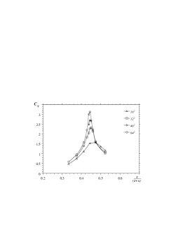
Figure 3: The specific heat versus bending rigidity from the Monte Carlo simulation of Ref. 24. The critical exponent $\alpha=0.4(1)$.

To gain some insight into the effect of a finer discretization of the embedding space we have generalized planar folding to folding on a $3d$ Face Centred Cubic (FCC) lattice.[25]

In the general $3$–dimensional folding problem, the local folding constraint (3) imposes only that the three tangent vectors around each face be in the same plane and have relative angles of $2\pi/3$. This, however, does not impose any constraint on the relative positions of the two planes corresponding to two adjacent faces, which may form some arbitrary continuous angle. As opposed to the $2d$ case, this then leads to a problem with continuous degrees of freedom.

To define a discrete model of folding in $3d$, one must allow only a finite number of relative angles between adjacent faces. More specifically, one may also impose that the link variables themselves take their values among a finite set of tangent vectors, now in ${\bf R}^{3}$. For symmetry reasons, we took this set of tangent vectors to be the (oriented) edges of a regular solid of ${\bf R}^{3}$, made of equilateral triangles only.

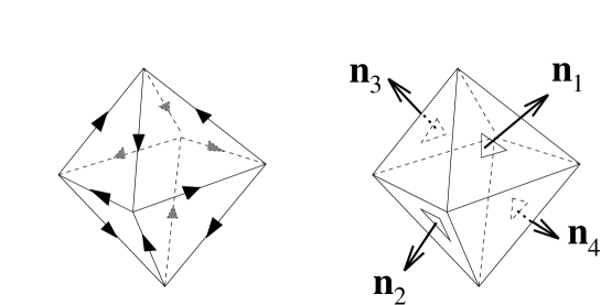
Figure 4: The oriented octahedron: the edges around each face form triplets of tangent vectors with vanishing sum. The four normal vectors ${\bf n}_{i}$, $i=1,2,3,4$, are represented on the corresponding outward oriented faces.

There are only three regular solids in ${\bf R}^{3}$ made of equilateral triangles: the tetrahedron, the octahedron and the icosahedron. The edges of the tetrahedron (resp. icosahedron), however, cannot be consistently oriented such that the corresponding tangent vectors satisfy (3) around each face. This is because each vertex is surrounded by an odd number 3 (resp. 5) of triangles. There is no such problem for the octahedron, as shown in Fig. 4. The $12$ links of the octahedron are oriented consistently to form $8$ triplets of tangent vectors with vanishing sum, corresponding to the $8$ faces of the octahedron. One may therefore consider the restricted $3d$ “octahedral folding” problem, where the tangent vectors are chosen from the set of 12 edge vectors of a regular oriented octahedron. In the folding process, the folding rule (3) imposes that the three links of a given face on the original triangular lattice are mapped onto one of the $8$ triplets of tangent vectors above. For a given triplet, the triangle can still be in $3!$ states corresponding to the $3!$ permutations of the three edges. Each triangle can therefore be in one of $48=8\times 6$ states.

The $8$ faces of the octahedron can be labelled as follows: we consider for each face its normal vector, pointing outward or inward according to the orientation of its tangent vectors on the octahedron (see Fig. 4). On the octahedron there are four alternating outward and inward oriented faces. The normal vectors to opposite faces are equal. This defines a set of four vectors ${\bf n}_{1}$, ${\bf n}_{2}$, ${\bf n}_{3}$ and ${\bf n}_{4}$, which furthermore satisfy the sum rule ${\bf n}_{1}+{\bf n}_{2}+{\bf n}_{3}+{\bf n}_{4}={\bf 0}$. Each face is labelled by its orientation (outward or inward) and its normal vector (1, 2, 3 or 4).

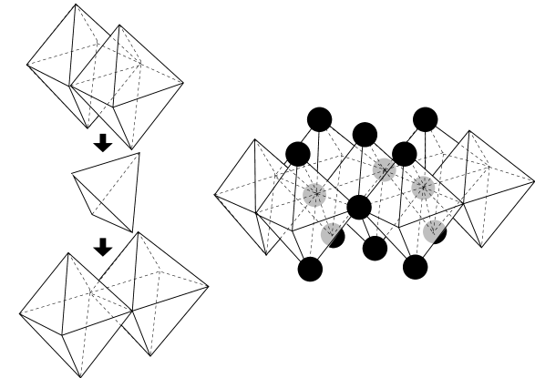
Figure 5: The FCC lattice viewed as a packing of $3d$ space with octahedra and tetrahedra.

The 12 oriented edge vectors of the octahedron are actually identical to the 6 edge vectors of a tetrahedron, now taken with both possible orientations. The four normal vectors above are also the normals to this tetrahedron. For each folding map, the image of the folded lattice in ${\bf R}^{3}$ lies therefore on a 3d FCC lattice, which consists of a packing of space by octahedra complemented by tetrahedra, as shown in Fig. 5. In this respect, the “octahedral folding” problem simply corresponds to discretizing the embedding space as an FCC lattice.

4.1 96–vertex Model

When stated in terms of tangent vectors, the $3d$ “octahedral folding” problem involves three types of constraints: face, link and vertex constraints. The first constraint, around each face, imposes that the three tangent vectors of a given triangle form one of the $8\times 6$ (ordered) triplets with vanishing sum. The second constraint, on each link, arises because two adjacent triangles share a common tangent vector. Given the state of one triangle, any adjacent triangle has one of its tangent vectors already fixed and thus is left with only $4=48/12$ possible states.

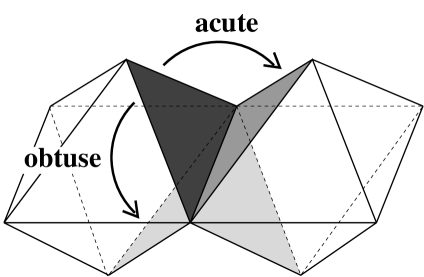
Figure 6: The four possible folding angles between two adjacent triangles. The neighbour of the dark triangle may (i) be itself on top of the dark triangle (complete fold), (ii) occupy the symmetric position in the same plane (no fold), (iii) lie on the same octahedron (i.e. form an obtuse angle) or (iv) lie on the same tetrahedron (i.e. form an acute angle).

They correspond simply to the four values for the relative angle between two neighbouring triangles, i.e. the angle between the normal vectors, depicted in Fig. 6. These four values are 0 (no fold: the triangles are side by side), $180^{\circ}$ (complete fold: the triangles are on top of each other), $\cos^{-1}(-1/3)\sim 109^{\circ}28^{\prime}$ (fold with acute angle: the two triangles lie on the same tetrahedron) and $\cos^{-1}(1/3)\sim 70^{\circ}32^{\prime}$ (fold with obtuse angle: the triangles lie on the same octahedron). Finally, there is a third constraint on the six successive folds around each vertex of the lattice: after making one loop, the same tangent vector must be recovered. Since the “metric constraint” is local, there are actually no constraints other than these three (face, link and vertex) constraints.

In the study of the $2d$ folding (3–colouring) problem, the face and link constraints are taken into account by going to ${\bf Z}_{2}$ spin variables $\sigma_{i}$ defined on the faces of the lattice. Ordering the colours cyclically, the spin is $+1$ (resp.  $-1$) if the colour increases (resp. decreases) from one link to the neighbouring one on the triangle, oriented counterclockwise. In this language, the actual folds take place exactly on the domain walls of the spin variable. Instead of having a ${\bf Z}_{3}$ colour variable per link, one is left with a ${\bf Z}_{2}$ spin variable per triangle. The vertex constraint translates into a constraint on the six spins $\sigma_{1},...,\sigma_{6}$ around each vertex of the lattice, namely that $\sum_{i=1}^{6}\sigma_{i}=0$ mod 3. This leads to 22 possible local spin configurations around each vertex, or equivalently, after removing the global ${\bf Z}_{2}$ degeneracy of reversal of all spins, to an 11–vertex model on the lattice.[14]

One may proceed in the same way for the $3d$ “octahedral folding” and account for the face and link constraints by expressing folded configurations in terms of two ${\bf Z}_{2}$ variables on the triangles. These variables will indicate the relative states of successive links around the face. One may then count the number of allowed hexagonal configurations around a vertex: this leads to a 96–vertex model. These vertices and the corresponding rules on the ${\bf Z}_{2}$ variables will be given below.

Let us label the $12$ edges of the octahedron as follows: each edge is shared by two adjacent faces, one outward and one inward oriented (see Fig. 4). We label the edges by the indices $(i,j)$, $1\leq i\neq j\leq 4$, when the normal vector for the outward face is ${\bf n}_{i}$ and the one for the inward face is ${\bf n}_{j}$. There are $12$ such couples $(i,j)$.

Figure 7: The transition from a link $(i,j)$ to a subsequent link $(k,l)$ is described by the two ${\bf Z}_{2}$ face variables $z$ and $\sigma$.

Consider now an elementary triangle of the lattice. Starting from one of its links $(i,j)$ the subsequent link $(k,l)$ counterclockwise must share a face with $(i,j)$ on the octahedron. This leads to the $4$ following possibilities, labelled by the ${\bf Z}_{2}$ face variables $z,\ \sigma\in\{\pm 1\}$:

$$\begin{array}[]{cl}z=+1:(i,j)\rightarrow(i,l),\ l\neq j,&\epsilon_{ijl}=-\sigma=\pm 1\\ z=-1:(i,j)\rightarrow(k,j),\ k\neq i,&\epsilon_{ijk}=+\sigma=\pm 1,\\ \end{array}$$ (5)

where $\epsilon_{ijk}=\sum_{l}\epsilon_{ijkl}$ is defined in terms of the totally antisymmetric tensor $\epsilon_{ijkl}$, equal to the signature of the permutation $(ijkl)$ of $(1234)$. The value $z=+1$ (resp. $z=-1$) indicates that the two tangent vectors share an outward oriented (resp. inward oriented) face on the octahedron. The spin variable $\sigma$ takes the value $+1$ (resp. $-1$) if $(k,l)$ follows (resp. precedes) $(i,j)$ on their common (oriented) face of the octahedron. The variable $\sigma$ also indicates whether the normal vector to the triangle (in the embedding space ${\bf R}^{3}$) is parallel ($\sigma=+1$) or antiparallel ($\sigma=-1$) to the corresponding normal vector of the octahedron.

Considering now two neighbouring triangles, the $4$ possible relative values $z_{2}/z_{1}$ and $\sigma_{2}/\sigma_{1}$ indicate which type of fold they form. The domain walls for the $z$ variable are the location of the folds which are either acute or obtuse, whereas those for the $\sigma$ variable are the location of the folds which are either complete or obtuse. The superposition of these two types of domain walls fixes the folding state of all the links, specifying the folding state of the lattice up to a global orientation.

The use of $z$ and $\sigma$ variables instead of the $12$ $(i,j)$ variables incorporates the face and link constraints. As in the $2d$ case, the vertex constraint is more subtle. Nevertheless, one can count the number of possible configurations around a vertex satisfying this constraint, i.e. the number of possible folded states of an elementary hexagon. Indeed the mapping (5) may be represented by a $12\times 12$ connectivity matrix $M_{(i,j),(k,l)}$ with $i\neq j$ and $k\neq l$:

$${M_{(i,j),(k,l)}=\delta_{ik}+\delta_{jl}-2\,\delta_{ik}\delta_{jl}\ .}$$ (6)

This matrix acts as a transfer matrix between two successive internal links of the hexagon. The number of configurations of a hexagon is simply given by: ${\rm Tr}(M^{6})=4608$, where the trace guarantees that the same link variable is recovered after one loop. These $4608$ configurations count as distinct all the foldings which are related by a global change of orientation of the hexagon in embedding space. The order of the resultant degeneracy is $48$, corresponding to $12$ choices for the first tangent on the octahedron times $4$ for the choice of the second from among its 4 neighbours (this latter choice corresponds to the $4$ choices of the $z$ and $\sigma$ variables on the corresponding triangle). This leaves us with $4608/48={\bf 96}$ distinct configurations.

4.2 Vertex Rules

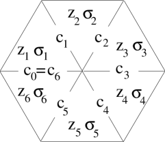
Figure 8: The six $z_{i}$ and $\sigma_{i}$ variables around a given vertex, and the colours $c_{i}$ of the interior links.

Consider an elementary hexagon of the triangular lattice. As shown in Fig. 8 each of its 6 triangles is labelled by $z$ and $\sigma$ variables. Let us also assign a colour $c_{i}$ to each link: $c_{i}=c_{0}+\sum_{j=1}^{i}\sigma_{j}\ {\rm mod}\ 3$. Geometrically each colour corresponds to one of the three orthogonal planes of the target octahedron (comprising four links). The vertex constraint arises from the requirement that six applications of the link mapping of Eq.(5) be the identity. By relating the link mappings to the elements of the tetrahedral group $A_{4}$ one finds two folding rules.[25] The first folding rule:

$${\sum_{i=1}^{6}\sigma_{i}=0\ {\rm mod}\ 3}$$ (7)

for the six spins around the central vertex of the hexagon is identical to the planar folding rule. In contrast with the $2d$ situation, the restriction (7) is not the only constraint. There is a second folding rule

$${\sum_{i=1}^{6}\frac{1}{2}(1-z_{i}z_{i+1})\delta(c_{i},c\ {\rm mod}\ 3)=0\ {\rm mod}\ 2\,:\quad c=1,2\ .}$$ (8)

The two folding rules (7) and (8) characterise the vertex constraint entirely.

Figure 9: The 96 vertices satisfying the two folding rules 7 and 8: no line corresponds to no fold, a thick line corresponds to a complete fold, a thin line corresponds to a fold with obtuse angle and a dashed line corresponds to a fold with acute angle. The degeneracy of each vertex under cyclic permutations of the links is indicated.

One finds $384=96\times 4$ vertex configurations (there is a $4$–fold global degeneracy under reversal of $z$ or $\sigma$). The $96$ folding vertices are displayed in Fig. 9 with the following conventions: no line corresponds to no fold; a thick line corresponds to a complete folding ($180^{\circ}$, flip of $\sigma$ only); a thin line corresponds to a fold with obtuse angle ($\cos^{-1}(1/3)\sim 70^{\circ}32^{\prime}$ between normal vectors, flip of both $\sigma$ and $z$) and finally a dashed line corresponds to a fold with acute angle ($\cos^{-1}(-1/3)\sim 109^{\circ}28^{\prime}$, flip of $z$ only). The degeneracy of each vertex under cyclic permutations of the links is also indicated.

Figure 10: Examples of $3d$ octahedral foldings of an elementary hexagon and the corresponding vertices of Fig. 9.

In Fig. 10 we display a few examples of vertices and the corresponding foldings in $3d$ space.

Figure 11: Bending Energy vs rigidity for $3d$ folding from a transfer matrix calculation on strips of width $L=2,3,4,5$ and $6$.

The $3d$ octahedral folding problem is thus precisely defined as a $96$–vertex model with the vertices of Fig. 9. Although the entropy of the $3d$ problem cannot be evaluated exactly it can be determined by a numerical transfer matrix calculation to be $q_{3d}\approx 1.43(1)$.[25] One can also derive various exact bounds on the entropy for $3d$ folding by relating it to dressed 3–colouring and $2d$ folding in an external staggered magnetic field.[25] The best bounds derived in this way, expressed numerically to three decimal places, are $1.436\leq q_{3d}\leq 1.589$.

We have also examined the phase diagram of $3d$ folding with bending energy. As for planar folding one finds a first-order phase transition to an ordered state at a critical value of the bending rigidity. The bending energy versus rigidity is shown in Fig. 11 for infinite strips of width $L=2,3,4,5$ and $6$. One sees quite clearly the emergence of a non-zero latent heat as the system size increases. This is confirmed by a finite-size scaling analysis of the peak of the specific heat plot: it grows linearly with system size, as characteristic of a first-order transition.

The planar and $3d$ folding models described here have also been studied in the hexagon approximation of the cluster variation method.[26] For planar folding this allows the incorporation of defects in the lattice and the study of the crossover from the pure Ising model to the pure folding problem. For $3d$ folding these authors also add a symmetry-breaking field to the model and find a first-order transition to a flat phase for any value of the symmetry breaking field.

In conclusion folding is a rich problem providing considerable insight into the phase structure of fluctuating membranes.

References

- [1] Scaling Concepts in Polymer Physics, P.G. de Gennes (Cornell University Press, Ithaca, NY, 1979).
- [2] Polymers in Solution: Their Modelling and Structure, G. des Cloiseaux and J.F. Jannink (Clarendon Press, Oxford, 1990).
- [3] D.R. Nelson in Statistical Mechanics of Membranes and Surfaces, edited by D. Nelson, T. Piran and S. Weinberg, Volume 5 of the Jerusalem Winter School for Theoretical Physics (World Scientific, Singapore, 1989).
- [4] D.R. Nelson, in Fluctuating Geometries in Statistical Mechanics and Field Theory, P. Ginsparg, F. David and J. Zinn-Justin eds. Les Houches Session LXII (Elsevier Science, The Netherlands, 1996).
- [5] D.R. Nelson and L. Peliti, J. Phys. France 48 (1987) 1085.
- [6] J.A. Aronovitz and T.C. Lubensky, Phys. Rev. Lett. 60 (1988) 2634.
- [7] E. Guitter, F. David, S. Leibler and L. Peliti, Phys. Rev. Lett. 61 (1988) 2949; J. Phys. France 50 (1989) 1787.
- [8] J.A. Aronovitz, L. Golubović and T.C. Lubensky, J. Phys. France 50 (1989) 609.
- [9] Y. Kantor, M. Kardar and D.R. Nelson, Phys. Rev. Lett. 57 (1986) 791; Phys. Rev. A 35 (1987) 3056.
- [10] F. David and E. Guitter, Europhys. Lett. 5 (1988) 709.
- [11] R.D. Pisarski, Phys. Rev. D 28 (1983) 2547.
- [12] A.M. Polyakov, Nucl. Phys. B 268 (1986) 406.
- [13] Y. Kantor and M.V. Jarić, Europhys. Lett. 11 (1990) 157.
- [14] P. Di Francesco and E. Guitter, Europhys. Lett. 26 (1994) 455.
- [15] R.J. Baxter, J. Math. Phys. 11 (1970) 784; J. Phys. A: Math. Gen. 19 (1986) 2821.
- [16] P. Di Francesco and E. Guitter, Phys. Rev. E 50 (1994) 4418.
- [17] M. Paczuski, M. Kardar and D.R. Nelson, Phys. Rev. Lett. 60 (1988) 2638.
- [18] Y. Kantor and D.R. Nelson, Phys. Rev. Lett. 58 (1987) 2774; Phys. Rev. A 36 (1987) 4020.
- [19] M. Baig, D. Espriu and J. Wheater, Nucl. Phys. B 314 (1989) 587.
- [20] J. Ambjørn, B. Durhuus and T. Jonsson, Nucl. Phys. B 316 (1989) 526.
- [21] R. Renken and J. Kogut, Nucl. Phys. B 342 (1990) 753.
- [22] R. Harnish and J. Wheater, Nucl. Phys. B 350 (1991) 861; J. Wheater and P. Stephenson, Phys. Lett. B 302 (1993) 447; J. Wheater, Nucl. Phys. B 458 (1996) 671.
- [23] M. Baig, D. Espriu and A. Travesset, Nucl. Phys. B 426 (1994) 575.
- [24] M. Bowick, S. Catterall, M. Falcioni, G. Thorleifsson and K. Anagnostopoulos, J. Phys. I (France) 6 (1996) 1321.
- [25] M. Bowick, P. Di Francesco, O. Golinelli and E. Guitter, Nucl. Phys. B 450 (1995) 463.
- [26] E. Cirillo, G. Gonnella and A. Pelizzola, Phys. Rev. E 53 (1996) 1479; Phys. Rev. E 53 (1996) 3253.