COMPRESSIBILITY, CAPACITANCE AND GROUND STATE ENERGY FLUCTUATIONS
IN A WEAKLY INTERACTING QUANTUM DOT
Abstract
We study the effect of electron-electron (e-e) interactions on compressibility, capacitance and inverse compressibility of electrons in a quantum dot or a small metallic grain. The calculation is performed in the random-phase approximation. As expected, the ensemble-averaged compressibility and capacitance decreases as a function of the interaction strength, while the mean inverse compressibility increases. Fluctuations of the compressibility are found to be strongly suppressed by the e-e interactions. Fluctuations of the capacitance and inverse compressibility also turn out to be much smaller than their averages. The analytical calculations are compared with the results of a numerical calculation for the inverse compressibility of a disordered tight-binding model. Excellent agreement for weak interaction values is found. Implications for the interpretation of current experimental data are discussed.
pacs:
PACS numbers: 71.55.Jv,73.20.Dx,71.27.+aI Introduction
The interplay between disorder and interactions is one of the most exciting topics in mesoscopic physics. Both factors play an important role in determining the change of the number of electrons in a mesoscopic system as the chemical potential of the system is changed. The investigation of this problem is especially timely since ground-state properties of disordered interacting systems have recently become experimentally accessible. For example, by measuring the spacings between the gate voltages for which a quantum dot connected to external leads exhibits conductance peaks, one can infer the inverse compressibility of the electron gas in the dot [1, 2, 3, 4]. Devices of this type have recently been used to measure the many-particle ground-state energy as a function of the number of electrons in a dot and large fluctuations (compared to the single electron level spacing) in this property were observed[3, 4, 5]. Large fluctuations have also been observed in earlier experiments in which the inverse compressibility of an insulating indium-oxide wire was measured [6].
In the absence of interactions the derivative of the chemical potential with respect to the number of electrons (i.e., the inverse compressibility, equal also to the second derivative with respect to of the ground state energy) of a system equals to the single-electron level spacing. It is well known that the single-electron level statistics in disordered systems are connected to the statistical properties of random matrices [7, 8, 9]. The level spacings exhibit fluctuations and therefore one expects that the inverse compressibility of different samples, as well as the inverse compressibility for the same sample at different chemical potentials, will also exhibit fluctuations of order of the single-electron mean level spacing . In the non-interacting regime there are many theoretical approaches which can be used to calculate these fluctuations, among them are the random matrix theory (RMT)[9], perturbative diagrammatic calculations [8] and the supersymmetry method [10, 11].
On the other hand, once electron-electron (e-e) interactions are included the situation becomes more complicated. In contrast to the high energy excitations of an interacting system for which a RMT description works very well (for example the high excitations of a nuclei[9] and of disordered interacting systems[12] ), The ground-state energy of an interacting system as a function of the number of particles can not be understood by means of RMT.
The average compressibility , as well as the average capacitance , are expected to decrease as result of interactions since it costs more energy to add particles into the system. This is somewhat similar to the situation for the average polarizability suppression by the e-e interactions [13, 14].
It is not a priori clear how the interactions will influence the fluctuations. Previously we have calculated the influence of e-e interactions on the sample-to-sample fluctuations of the polarizability [15]. By analogy one might expect that the relative magnitude of the compressibility and capacitance fluctuations should be suppressed.
The average inverse compressibility is expected to increase as a function of interaction strength for repulsive interactions. From the experimental evidence it seems that the fluctuations in the inverse compressibility is proportional to [3, 4, 5, 6]. From numerical calculations one learns that for strong interactions the mean root square of the inverse compressibility are proportional to its average[5], with a proportionality constant of about for a very wide range of interactions and disorder strengths. However, it is evident that for weak interactions this ratio can not be constant. Our goal is to study the behavior of the inverse compressibility for weak interactions, and to understand the transition to the strong interaction regime.
In this paper we extend the perturbative diagrammatic calculations to include e-e interactions. The average compressibility, capacitance and inverse compressibility as a function of the interaction strength are calculated. The fluctuations in the compressibility and capacitance are found to be strongly suppressed by the e-e interactions. The fluctuations in the the inverse compressibility of the sample can also be deduced from the fluctuations in the compressibility. It turns out that the fluctuations in the inverse compressibility, while not suppressed are relatively small.
This is checked by an exact diagonalization numerical study of an interacting, spinless, disordered tight-binding model for nearest-neighbor interactions as well as for long-range Coulomb interactions. For weak interactions the numerical results follow the perturbative calculation. As may be expected from earlier studies, [5] deviations appear as the strength of interaction is increased. Thus, a transition from weak-interaction behavior of the fluctuations to strong-interaction behavior is evident. In the end we discuss the significance of these results for the interpretation of the experiments.
II Averaged Compressibility
The compressibility may be written in terms of the exact Green function of the system as:
| (1) |
where is the Fermi energy of the system, is the number of particles. Given the Hamiltonian , the exact Green function can be written as
| (2) |
For the non-interacting case Eqs. (1,2) take the form
| (3) |
where is the volume and
| (4) |
Here () is the n-th eigenvector (eigenvalue) of the system. This defines the density of states at the Fermi energy
| (5) |
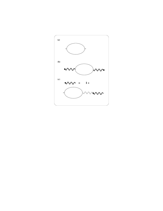
According to Eq. (5) in order to add one electron to the system the Fermi energy should change by . This can be also represented in a diagrammatic perturbation theory by the diagram shown in Fig. 1(a) corresponding to
| (6) |
where denotes an average over different realizations of disorder.
Now let us discuss the influence of e-e interactions on the averaged compressibility. One would expect that repulsive e-e interactions will reduce the compressibility since it costs additional interaction energy to insert an electron into the system. We begin by investigating the role of short range interactions represented by
| (7) |
and
| (8) |
where is a dimensionless coupling constant and ; here is the range of the interaction and is the systems dimensionality. The compressibility in the interacting case may be represented by the diagrams shown in Fig. 1(b), corresponding to
| (9) |
where is the result of summing the diagrammatic series shown in Fig. 1(c). For a short range interaction
| (10) |
Inserting the result for into Eq. (9) one obtains
| (11) |
Thus, the additional energy needed to add an electron due to the e-e interactions (the charging energy) is . This is exactly the result expected if one assumes a constant density of electrons in the system.
The calculation of the compressibility for the long-ranged Coulomb interaction can be performed along similar lines. For the Coulomb interaction
| (12) |
and for an infinite system
| (13) |
(where and ) which for future convenience in the numerical simulations may also be written as . As can be seen in Eq. (9) the zero mode () determines the behavior of the average compressibility. Therefore, one must treat the zero mode carefully, since simply inserting the infinite system value of the interaction for will lead to no compressibility, i.e., infinite capacity. The zero component of the Fourier transform for a finite system is equal to
| (14) |
where
| (15) |
is a numerical constant which depends on the geometry. Thus repeating the summation of the diagrammatic series shown in Fig. 1(c) one obtains
| (16) |
where , which is the usual random phase approximation (RPA) for the e-e interactions. Using the above result in Eq. (9) results in
| (17) |
Therefore, the compressibility tends to its non-interacting value for (i.e., large screening length, possible for example in very small semiconducting grains) and to of its non-interacting value for (metallic grains).
III Fluctuations in Compressibility
In this section we shall calculate the fluctuations in the compressibility in the presence of e-e interactions. For the non-interacting electrons the fluctuations are expected follow the Wigner-Dyson statistics. As was noted in Ref. [8], in order to obtain the Wigner-Dyson statistics in the perturbative diagrammatic calculation one must insert a cut-off in energy (or temperature) of order of the single electron level spacing . Explicitly the fluctuations can be calculated using the diagrams appearing in Fig. 2(a), which correspond to
| (18) |
where is the Matsubara frequency and is the temperature. is the Fourier transform of the diffusion propagator which is the solution to the equation
| (19) |
with reflective boundary conditions , where is the normal to the sample edge. For a rectangular grain of dimensions , the solution is
| (20) |
where , (for a two dimensional system the component drops out) and . After inserting the value of diffusion propagator given in Eq. (20) one is left with the following summation:
| (21) |
The most significant contribution comes from the zero mode () resulting in
| (22) |
The fluctuations in the interacting case are represented by the diagrams shown in Fig. 2(b) corresponding to
| (23) |
where is given by Eqs. (10,16). Note that appears in the power of four, which is the the result of the fact that when two RPA lines intersect, four lines appear. For the short range interactions we obtain
| (24) |
Thus, the fluctuations in the compressibility are suppressed by the interactions as compared to the non-interacting value. Even the relative fluctuations (defined as the fluctuations in the compressibility divided by the averaged compressibility) are suppressed by the interactions. According to Eq. (11):
| (25) |
A similar situation exists also for the Coulomb interactions. By using the value of given in Eq. (16) one obtains
| (26) |
and (using Eq. (17))
| (27) |
Thus, for the relative fluctuations are the same as in the non-interacting case, while the relative fluctuations are suppressed by a factor of . It is important to note that for most metallic and semiconducting samples the above relation holds since is of the order of the Fermi momentum, i.e., for a grain with electron.
IV Capacitance
From the experimental point of view, capacitance measurements is one of the most accessible methods to investigate the spectral properties of quantum dots and grains[2]. Therefore, it is interesting to connect the fluctuations in the compressibility to fluctuations in the capacitance for interacting disordered systems. The capacitance of a grain may be related to its chemical potential in the following way:
| (28) |
which is equivalent to
| (29) |
when and thus one may write the average capacitance as
| (30) |
After inserting the calculated compressibility for the long-range Coulomb interaction (Eq. (17)) one obtains
| (31) |
which is the expected purely geometrical value of the capacitance.
The fluctuations in the capacitance can be expressed via the fluctuations in the compressibility in the following way
| (32) |
which after inserting Eq.(27) results in
| (33) |
Thus when the fluctuations in the capacitance are much smaller than the average capacitance.
V Inverse Compressibility
As mentioned briefly in the introduction, the inverse compressibility of a quantum dot can be deduced from measurements of the spacings between consecutive gate voltages for which the conductance through the dot peaks. The spacings in the gate voltage are proportional to the difference between the chemical potential of and electrons [5] denoted by , which may be related to the ground state energies in the following way:
| (34) |
where is the ground state energy of the dot populated by electrons. In the continuum limit , i.e., the experiment actually measures the discrete limit of the inverse compressibility.
The first step in connecting the results obtained from the compressibility calculations to the behavior of is to relate to . With no loss of generality one can write
| (35) |
and
| (36) |
which if one assumes a well behaved distribution of the compressibility will result in
| (37) |
In a similar manner
| (38) |
These relations are valid as long as . From Eqs. (11,17) and (24,26) it can be seen that this condition is usually fulfilled since . The above condition also holds in the non-interacting metallic regime for which the usual diagrammatic expansion is valid.[17, 18] Thus
| (39) |
for short range interactions and
| (40) |
for Coulomb interactions. The fluctuations in both cases are equal to
| (41) |
From Eqs. (39,40) it is clear that grows proportionally to the interaction strength ,while the fluctuations are independent of the interaction strength.
This behavior implies that while the e-e interactions tend to shift the distribution of the inverse compressibility the width of the distribution will not change significantly[19].
The results for could also be anticipated from a simple assumption on the distribution of the electron density of the ground-state. The electrostatic energy needed to add an electron to a system of electrons is given by
| (42) |
where is the density of the electrons already in the system, and is the density of the additional electron. Assuming that both densities are uncorrelated, and that on the average and , the average electrostatic energy needed to add an electron is
| (43) |
which for short-range interactions results in and for the Coulomb interactions . Since under these assumptions , one immediately obtains Eqs. (39,40), which is the classical limit of the Coulomb blockade.[20]
Also the fluctuations in the inverse compressibility may be deduced from similar assumptions, resulting in
| (44) |
for both short and long range interactions. Thus, the fluctuations in the charging energy are , This leads to the conclusion that there is no additional contribution to the inverse compressibility fluctuations beyond the fluctuations in , in agreement with Eq. (41).
Therefore, we expect that the results presented in the previous sections will hold as long as the RPA assumptions hold, i.e., , where is the Fermi velocity.
VI Numerical Calculation of the Inverse Compressibility
In this section we shall numerically test the properties of the inverse compressibility. Of course, in a numerical calculation we can only compute the discrete form of , i.e, as a function of the strength of e-e interactions in the system.
As a model system we chose a system of interacting electrons on a 2D cylinder of circumference and height , which has been previously used in the study of the influence of e-e interactions on persistent currents. [21] The model Hamiltonian is given by:
| (45) |
where is the fermionic creation operator, is the energy of a site (), which is chosen randomly between and with uniform probability and is a constant hopping matrix element. is the interaction part of the Hamiltonian given by:
| (46) |
for the short range interactions (where denotes nearest-neighbor pair of sites) and
| (47) |
for the Coulomb interaction, where is the lattice constant.
For a sample of sites and electrons, the number of eigenvectors spanning the many body Hilbert space is . The many-body Hamiltonian may be represented by an matrix which is numerically diagonalized for different values of the e-e interaction. Here we consider a , and lattices with sites correspondingly. For each value of the average and fluctuations of are calculated. To obtain in each case for , and are calculated. For the largest system considered (,) the calculation of the ground-state energy corresponds to diagonalizing a matrix. We chose for which this system is in the metallic regime [21] and average the results over realizations for each value of interaction strength for the and cases and realizations for .
The results for and are given in Fig. 3a for the short-range interactions and in Fig. 3b for the Coulomb interaction. It can be seen that in both cases increases linearly for low values of while remains constant. This is in qualitative agreement with Eqs. (39 - 41). In order to obtain also quantitative agreement one must take into account some finer details. For one must consider the fact that the calculations were performed on a lattice. For short range interactions, one should replace in Eq. (39) by where the average number of nearest neighbors, , depends on due to the different ratio of sites close to the boundaries, where for , correspondingly. Using the values of the single electron spacings for in Eq. (39) results in the curves plotted in Fig. 3(a) for . One can see a good fit up to . For the long range interactions in our lattice system one should replace the integration in Eq. (15) by a summation, i.e. , which results in corresponding to . After incorporating and in Eq. (40) one obtains the curves plotted in Fig. 3b. An excellent fit is seen up to . The exact value of is deduced from RMT and plotted in Fig. 3. It can be seen that this prediction is also confirmed for weak interactions [22].
It is possible to observe what is the influence of the e-e interactions on the full distribution of . In Fig. 4 the distribution for the non-interacting case () is compared with the distribution for in the long range interaction case. As can be seen in Fig. 3b, for this value of interaction strength no significant change in the second moment of the distribution is expected, and indeed the width of the distributions is almost identical. On the other hand, higher moments seem to be influenced by the e-e interactions resulting in changes in the tails of the distribution. The effect of interactions on the higher moments of the merits further studies.
As has been mentioned in Ref. [5], and discussed in the previous section, we expect the analytical results based on the RPA approximation to hold as long as no correlations develop in the electron density. Following Ref. [5] we define a two point correlation function:
| (48) |
where
| (49) |
In Fig. 5 we present the correlation (which corresponds to a pair of diagonal sites) for the long-range interactions as function of the interaction strength. Under the RPA assumptions we expect . As can be seen there is some correlation as result of the boundaries even without e-e interactions. As the interaction strength increases there is no dramatic change in up to and then one sees a strong deviation. A similar behavior can be seen for the short range interactions where the deviation appear at . This agrees well with the values of interaction for which the numerical results depart from the RPA analytical calculations.
One can roughly estimate the strength of interaction for which these correlations should appear. As mentioned in the previous section, we expect the RPA approximation to hold while , which for long range interactions corresponds to and for short range interactions to . This is surprisingly close to the values for which deviations from RPA theory are seen numerically.
VII Discussion
The main conclusion that follows of the previous sections is that the RPA approximation fails to explain the large fluctuations in the inverse compressibility seen in the experiment [3, 4, 5]. Under the assumptions of an RPA treatment of the e-e interactions the fluctuations are proportional to the single electron mean level spacing, therefore independent of the strength of the e-e interactions. In contrast, experiments show that the fluctuations are substantially larger than the mean level spacing, and seem to be about 15 percent of the average inverse compressibility.
Actually, one could have anticipated the failure of the RPA calculation for the experimental realizations, since their densities are too low for the RPA approximation to remain valid. For a 2DEG quantum dot one may rewrite the condition for which the RPA fails as , where is the electron density in the dot and is the Bohr radius, which in GaAs is . Thus one expects RPA to fail at densities . In all of the recent experiments for which large fluctuations were observed [3, 4, 5] the 2DEG density is about , and the density in the dot is probably even lower.
The large fluctuations in the inverse compressibility are caused by spatial fluctuations in the electron density which are not taken into account in the RPA approximation [5]. It is important to note that although the charge distribution becomes inhomogeneous when the electron density is still much higher than the one critical for Wigner crystallization. Thus the experiments are apparently in an intermediate range of densities (or intermediate e-e interaction strength). In this regime RPA approximation does not hold anymore and some density correlations do appear, however the systems are still very far from the Wigner crystallization.
Note that in the case of large dimensionless conductance that was considered in this paper we found no influence of the disorder on the structure of Coulomb blockade peaks. For different physical reasons fluctuations of the order of the inverse compressibility may also appear in the localized regime.[23]
Finally, it is also interesting to compare the fluctuations in the compressibility to the fluctuations in the polarizability.[15] Although the calculation of both quantities show many similar features, there is one crucial difference. The main contribution to the fluctuations in the compressibility comes from the zero-mode, which corresponds in the non-interacting case to the single electron level fluctuations. In the polarizability, there is no contribution from the zero mode, and the fluctuations stem from the other modes, which correspond to density fluctuations. This results in the fact that the relative polarization fluctuations are smaller than the relative compressibility fluctuations by a factor .
Acknowledgments
We would like to thank A. Auerbach, M. Field, Z. Ovadyahu, B. Shklovskii, U. Sivan and D. A. Wharam for useful discussions. R.B. would like to thank the US-Israel Binational Science Foundation for financial support.
REFERENCES
- [1] For recent reviews see: M. A. Kastner, Rev. Mod. Phys. 64, 849 (1992); U. Meirav and E. B. Foxman, Semicond. Sci. Technol. 10, 255 (1995).
- [2] R. C. Ashoori, Nature 379, 413 (1996).
- [3] A. M. Chang, H. U. Baranger, L. N. Pfeiffer, K. W. West and T. Y. Chang, Phys. Rev. Lett. 76, 1695 (1996).
- [4] J. A. Folk, S. R. Patel, S. F. Godijn, A. G. Huibers, S. M. Cronenwett, C. M. Marcus, K. Campman and G. Gossard, Phys. Rev. Lett. 76, 1699 (1996); C. M. Marcus, J. A. Folk, S. R. Patel, S. M. Cronenwett, A. G. Huibers, K. Campman and G. Gossard (preprint).
- [5] U. Sivan, R. Berkovits, Y. Aloni, O. Prus, A. Auerbach and G. Ben-Yoseph, Phys. Rev. Lett. 77, 1123 (1996).
- [6] V. Chandrasekhar, Z. Ovadyahu and R. A. Webb, Phys. Rev. Lett. 67, 2862 (1991).
- [7] L. P. Gorkov and G. M. Eliashberg Zh. Eksp. Teor. Fiz. 48, 1407 (1965) [Sov. Phys. JETP 21, 940 (1965)].
- [8] B. L. Altshuler, and B. I. Shklovskii, Zh. Eksp. & Teor. Fiz. 91, 220 (1986) [Sov. Phys. JETP 64,127 (1986)].
- [9] M. L. Mehta, Random matrices (Academic Press, San-Diego, 1991).
- [10] K. B. Efetov, Adv. Phys.32, 53 (1983).
- [11] J. J. M. Verbaarschot, H. A. Weidenmuller, and M. R. Zirnbauer, Phys. Repts. 129,367 (1985).
- [12] R. Berkovits, Europhys. Lett. 25, 681 (1994); R. Berkovits and Y. Avishai, J. Phys. Condens. Matter 8, 391 (1996).
- [13] S. Strassler, M.J. Rice and P. Wydner, Phys. Rev. B 6, 2575 (1972).
- [14] M. J. Rice, W. R. Schneider, and S. Strassler, Phys. Rev. B 8, 474 (1973).
- [15] R. Berkovits and B. L. Altshuler, Europhys. Lett. 19, 115 (1992); Phys. Rev. B 46, 12526 (1992).
- [16] B. L. Altshuler and A. G. Aronov, in Electron-electron interactions in disordered systems Ed. A. L. Efros and M. Pollak (North-Holland, 1985)
- [17] B. L. Altshuler, Y.Gefen and Y. Imry Phys. Rev. Lett. 66, 88 (1991); A. Schmidt (1991).
- [18] A. Kamenev, B. Reulet, H. Bouchiat and Y.Gefen, Europhys. Lett. 28, 391 (1994).
- [19] On the other hand, since we did not calculate higher moments, it is possible that the tail of the distribution will change as function of the interaction strength.
- [20] D. V. Averin and K. K. Likhraev in Mesoscopic phenomena in solids Ed. B. L. Altshuler, P. A. Lee and R. A. Webb (North-Holland, 1991)
- [21] R. Berkovits and Y. Avishai, Europhys. Lett. 29, 475 (1995); Phys. Rev. Lett. 76, 291 (1996).
- [22] Some deviations occur for , probably because for this larger lattice size the system is closer to the Anderson transition.
- [23] A. L. Efros and B. Shklovskii, in Electron-electron interactions in disordered systems Ed. A. L. Efros and M. Pollak (North-Holland, 1985); F. Pikus and B. Shklovskii (APS March meeting abstract, 1996)