Persistent currents in continuous one-dimensional disordered rings within the Hartree–Fock approximation

Abstract

We present numerical results for the zero temperature persistent currents carried by interacting spinless electrons in disordered one dimensional continuous rings. The disorder potential is described by a collection of $\delta$-functions at random locations and strengths. The calculations are performed by a self-consistent Hartree-Fock (H-F) approximation. Because the H-F approximation retains the concept of single-electron levels, we compare the statistics of energy levels of noninteracting electrons with those of interacting electrons as well as of the level persistent currents. We find that the e-e interactions alters the levels and samples persistent currents and introduces a preffered diamagnetic current direction. In contrast to the analogous calculations that recently appeared in the literature for interacting spinless electrons in the presence of moderate disorder in tight-binding models we find no suppression of the persistent currents due to the e-e interactions.

]

I INTRODUCTION

The prediction of Büttiker, Imry and Landauer [1] that a persistent current (PC)[2, 3] can be observed in a disordered normal metal mesoscopic ring threaded by a magnetic flux, although this ring has a finite resistance due to elastic scattering, has attracted much recent attention [4, 5, 6, 7, 8, 9]. The elastic scattering, due to disorder, reduces the amplitude of this current. The detection of the effect in three different experiments, by measuring the magnetic signal of the PC, has stimulated a great deal of theoretical interest in particular because of the large magnetic response that was measured. The measured amplitude of the PC, although some of the samples are clearly in the disordered diffusive regime, is of the same magnitude as that calculated for electrons in a clean ring.

The simultaneous measurement [10] of the magnetic response of $10^{7}$ metallic Cu rings yields PC amplitude which is one order of magnitude larger than predicted by single-electron calculations which take into account the elastic scattering due to the disorder. This rised the question of the source of such large magnetic response of an ensemble of rings which are in the diffusive regime of disorder. The experimental signals of three single Au rings [11] of different geometries were found to be up to two orders of magnitudes larger than the prediction of such single electron theory. On the other hand, the response [12] of a 2D semiconducting ring in the ballistic regime of disorder and at a very low electronic density agrees well with the theoretical predictions of the single electron theory. These experimental findings rise the question whether the discrepancies between single electron theory and the observed behavior of the PC can be understood as a consequence of neglecting the e-e interactions in the presence of disorder. This question is part of a more general problem of the influence of electronic interactions in the presence of disorder on the properties of mesoscopic systems which is in the center of many recent studies, such as polarizability fluctuations [13], quasiparticle life times in quantum dots [14] and the metal-insulator transition [15].

There have been many attempts to investigate the influence of e-e interactions on the PC. Analytical calculations were mainly restricted to perturbation theories[16] and to renormalization treatments of Luttinger liquid models [17], which have shown that some enhancement of the PC due to the e-e interaction is possible. Exact numerical diagonalization studies of spinless interacting electrons for 1D [18, 19] as well as for 2D [20] tight-binding (TB) models were performed. In 1D systems for long range Coulomb interaction the PC is weakly enhanced for strong disorder (i.e., for the localized regime) and medium strength of interactions. But for weak disorder the current is suppressed at any strength of the interaction and filling factor [18]. Also for any strength of short range e-e interactions, even far from half filling, the PC has shown a decrease[19]. On the other hand, for 2D systems the PC is significantly enhanced in the diffusive regime [20]. Although these studies are useful in pointing towards the general influence of the e-e interactions they are restricted, due to exponential expansion of the Hilbert space with sample size, to samples of small number of sites (about six to twenty). This complex behavior has its origin in the interplay between two different physical effects. While the disorder creates fluctuations in the electronic density leading eventually to localization, the e-e interaction is expected to reinforce the tendency for local charge neutrality which counteracts the influence of disorder. In the H-F approximation this is realized by the effective potential which is expected to lead to an increase in the PC amplitude. On the other hand the Mott-Hubbard transition[21] reduces the current amplitude because the e-e interaction opens a gap at the middle of the conduction band leading to an insulating –not metallic– behavior of a half filled band.

It is interesting to examine the PC behavior in the H-F approximation because exact analytical consideration of interaction in the presence of disorder is a very difficult task. Even perturbative calculations are not conclusive [16]. On the other hand exact numerical diagonalization is limited to small number of sites and electrons. But using the H-F approximation has the advantage of the possibility to handle much larger systems. It has also the possibility to differentiate between different influences of the e-e interactions which may lead to an enhancement of the PC. Further it retains the concept of single electron levels in a meaningful way. This enables one to employ the considerable existing knowledge on statistical properties of single electron energy levels in disordered systems [22] for studying the influence of e-e interactions. One is also able to study the behavior of the current for different regimes of disorder since as the single electron energy becomes higher the effective disorder for these energies is weaker.

Kato and Yoshioka [23] were the first to deal with large 1D TB system of 100 sites and about half filling in the frame work of the self consistent H-F approximation for long range interaction. They have found that for any value of disorder the electronic interactions further suppress the PC and do not counteract the effect of disorder. This difference with the results of 1D exact diagonalization is due to the fact that the HF approximation for spinless electrons does not smear the density fluctuations which is essential to obtain an enhancement of the current in the localized regime. For spinless electrons in two[24] and three[25] dimensional TB rings the HF calculations show some enhancement of the average current for Coulomb interactions in the diffusive regime. But if the spin is taken into account the HF approximation shows a large enhancement of the PC[26]. The reason is that including the spin degrees of freedom adds a dominant contribution to the direct term. In fact, this effect can be seen even for first order perturbation theory[27, 28]. Thus, for the case where spin is taken into account, the HF approximation does describe the appearance of local charge neutrality due to interactions.

The main goal of this paper is to compare the PC behavior of interacting spinless electrons in continuous disordered rings with that behavior in TB rings that recently appeared in the literature [18, 19, 23]. For these TB rings in the moderate regime of disorder it was found that e-e interaction further suppresses the PC because of the Mott-Hubbard transition which does not seem to be relevant for electrons in continuous rings. The difference in the behavior of the PC is a measure for the importance of the difference between continuous and discrete models. The difference between a model with no discrete symmetries and the TB model has been suggested in Ref.[29] and here we shall examine this difference for a well defined Hamiltonian.

The rest of the paper is organized as follows: in section II we present the model for independent electrons and interacting electrons within the self consistent HF approximation. In section III we discuss the numerical results, and in section IV we derive our conclusions.

II Model of electrons in disordered 1D continuous rings.

A Non interacting electrons

Let $R$ be the radius of the continuous 1D ring, $\theta$ the coordinate along the ring, $m_{e}$ is the electron mass, $e$ its charge, $\phi$ the flux threading the ring and $\phi_{0}\equiv{hc\over e}$ the flux quantum. For completeness and further reference let us restate some basic facts. Defining the disorder potential as $V_{dis}(\theta)$ the Schrödinger equation (in energy units ${\hbar^{2}\over m_{e}R^{2}}=1$ ) for non-interacting electrons is:

$${1\over 2}\left({\partial\over i\partial\theta}+{\phi\over\phi_{0}}\right)^{2}\Psi(\theta)+V_{dis}(\theta)\Psi(\theta)=E\Psi(\theta),$$ (1)

where the boundary conditions (BC) are periodic

$$\Psi(\theta+2\pi)=\Psi(\theta).$$ (2)

The substitution[2] $\;\Psi(\theta)=\psi(\theta)e^{-i{\phi\over\phi_{0}}\theta}\;$ yields a wave equation of the Bloch type[1]

$$-{1\over 2}{\partial^{2}\over\partial\theta^{2}}\psi(\theta)+V_{dis}(\theta)\psi(\theta)=E\psi(\theta),$$ (3)

which now has the modified BC

$$\psi(\theta+2\pi)=\exp{(i2\pi{\phi\over\phi_{0}})}\psi(\theta).$$ (4)

An exact eigenstate of energy $E_{l}$ carries PC $i_{l}$

$$\begin{array}[]{c}i_{l}=-c{\partial\over\partial\phi}E_{l}\equiv-{\hbar\over m_{e}R}<\Psi_{l}|\left({\partial\over i\partial\theta}+{\phi\over\phi_{0}}\right)|\Psi_{l}>\\ =-{\hbar\over m_{e}R}<\psi_{l}|{\partial\over i\partial\theta}|\psi_{l}>\end{array}$$ (5)

(where numerically we use dimensionless energy and dimensionless current $-{\partial E\over\partial{\phi\over\phi_{0}}}$). We stress that $\Psi_{l}(\theta)$ are the electronic wave functions which are exactly periodic for any value of $\phi$. This fact will be important when we consider interactions. For $V_{dis}(\theta)\equiv 0$ the electronic functions are $\Psi_{l}(\theta)={1\over\sqrt{2\pi}}\exp{(il\theta)}$ with $l=0,\pm 1,\pm 2,...$ and the spectrum is $E_{l}={1\over 2}x_{l}^{2}$ with $x_{l}\equiv l+{\phi\over\phi_{0}}.$ For our model we have chosen

$$V_{dis}(\theta)=\sum_{j=1}^{N_{s}}\lambda_{j}\delta(\theta-\theta_{j})$$ (6)

where the locations $0\leq\theta_{j}\leq 2\pi$ and strength $-\Lambda\leq\lambda_{j}\leq\Lambda$ of the individual $j$-th scatterer are random with the appropriate probabilities: $P_{{}_{\theta}}(\theta_{j})={1\over 2\pi}$ and $P_{{}_{\lambda}}(\lambda_{j})={1\over 2\Lambda}$. $N_{s}$ is the total number of scutterers in the ring. $V_{dis}(\theta)$ produces characteristics of disordered samples as was discussed by Imry and Shiren[30] while truncating the Hilbert space. For non-interacting electrons one can exactly find the spectrum and eigen functions by means of a numerical transfer matrix technique. A transfer matrix that “propagates” the solution of eq.(3) from the left of the $j$-th scatterer to the left of the next $j+1$-st scatterer is given by:

$${\bf T}_{j}=\left(\begin{array}[]{cc}(1+{\lambda_{j}\over ix})e^{ix(\theta_{j+1}-\theta_{j})}&{\lambda_{j}\over ix}e^{ix(\theta_{j+1}-\theta_{j})}\\ -{\lambda_{j}\over ix}e^{-ix(\theta_{j+1}-\theta_{j})}&(1-{\lambda_{j}\over ix})e^{-ix(\theta_{j+1}-\theta_{j})}\end{array}\right)$$ (7)

where the exponents contain the effect of free propagation of waves between the scutterers. If we denote as ${\bf v}_{j}$ a two component vector in which the upper component corresponds to the amplitude of the forward propagating wave $e^{ix\theta}$ and the lower component to $e^{-ix\theta}$ then ${\bf v}_{j+1}={\bf T}_{j}{\bf v}_{j}$.

The concepts of localization length $\xi$ and the Landauer conductance, which are very useful in the study of open systems, can be defined by comparing eq.(7) with the general form of a transfer matrix:

$${\bf T}=\left(\begin{array}[]{cc}1/t^{*}&-(r/t)^{*}\\ -(r/t)&1/t\end{array}\right).$$ (8)

($t$ and $r$ the complex transmission and reflection coefficients obeying $|r|^{2}+|t|^{2}=1$). One can now analytically find $\xi$ as a function of energy and also find the appropriate scaling[31] behavior of the fluctuations of the Landauer resistance $\rho\equiv{|r|^{2}\over|t|^{2}}$ (or conductance $g\equiv 1/\rho$), where $N_{s}$ plays the role of the length scale of the conductor[32].

FIG. 1.: (a) Scaling behavior of the disorder average Landauer resistance $<\rho>$ as a function of the number of scatterers $N_{s}$ for an open chain of scatterers at weak disorder ($\Lambda=5$, $E=5000$, see text). (b) Scaling behavior of $<\ln(1+\rho)>$ of an open chain at strong disorder ($\Lambda=20$, $E=200$). The slope defines the inverse localization length ${1\over\xi}$. The empty symbols in (a) and (b) are our analytical estimates by eqs.(9) and (10) respectively, the full symbols are results of numerical simulations of 200 realizations.

For weak disorder, where $\rho_{j}\equiv{x^{2}\over\lambda_{j}^{2}}<<1,$ and small $N_{s}$ one expects an Ohm law behavior, i.e., disorder averaging should give $<\rho>\sim<\rho_{1}>N_{s}$ ($<\rho_{1}>$ is the average Landauer resistance of an individual scatterer). One finds

$$<\rho>\sim{\Lambda^{2}\over 3x^{2}}N_{s},$$ (9)

as long as $<\rho>$ is of order unity or smaller. A comparison of numerical results with the above equation is presented in Fig.1a.

Because of localization, for strong disorder or at any large enough $N_{s}$ (where $1<<\;<\rho>$) we expect $<\ln(1+\rho)>\sim{1\over\xi}N_{s}$ . In our case we analytically calculate $\xi$ to be

$$\xi^{-1}\equiv<\ln(1+\rho_{1})>=\ln(1+{\tilde{\Lambda}}^{2})-2+{2\over{\tilde{\Lambda}}}\tan^{-1}{\tilde{\Lambda}}$$ (10)

where ${\tilde{\Lambda}}\equiv{\Lambda\over x}$ and $\rho_{1}$ is the resistance of an individual scatterer. This result is confirmed by numerical calculations presented in Fig.1b where the slope is the inverse localization length.

Let us now return to the discussion of PC in the closed ring. The discrete spectrum and eigen functions of the ring can be found using the definition of the transfer matrix (eq. (7)) and the BC (eq. (4)) as an eigenvalue equation:

$$\prod_{j=1}^{N_{s}}{\bf T}_{j}{\bf v}_{1}=e^{2\pi i{\phi\over\phi_{0}}}{\bf v}_{1}.$$ (11)

It is enough to deal with the real (or imaginary) part of the last eigenvalue condition[33] in order to obtain the eigen values because the other part is automatically fulfilled. The case of $N_{s}=1$ at any strength of $\lambda$ can easily be solved. For $1<<N_{s}$ and appreciable strength of $\lambda_{j}$ the current can be calculated numerically and is found to be suppressed by many orders of magnitudes due to localization.

For a given disorder the total current[34] in an isolated (canonical) sample is the sum of the currents of all the occupied levels in the ring, which for $N_{e}$ electrons at zero temperature corresponds to:

$$I_{c}=\sum_{l=1}^{N_{e}}i_{l}.{ic}$$ (12)

For a sample connected to a reservoir (grand canonical) the sum is over all levels having energies lower than a given chemical potential $\mu$:

$$I_{g}=\sum_{E_{l}\leq\mu}i_{l}.$$ (13)

B Interacting electrons

We include $e-e$ interaction within the self consistent HF approximation. In analogy to the notations in eqs.(1) – (4) our equation for the new HF single particle wave function $\psi(\theta)$ reads:

$$\begin{array}[]{l}-\;{1\over 2}{\partial^{2}\over\partial\theta^{2}}\psi(\theta)+V_{dis}(\theta)\psi(\theta)\\ \\ +\;{R\over r_{0}}[{-N_{e}\over 2\pi}\int_{0}^{2\pi}{d\theta^{\prime}\over\sqrt{(\theta-\theta^{\prime})^{2}+\epsilon^{2}}}\psi(\theta)\\ \\ +\;\int_{0}^{2\pi}{\sum_{l=1}^{Ne}|\Psi_{l}(\theta^{\prime})|^{2}\over\sqrt{(\theta-\theta^{\prime})^{2}+\epsilon^{2}}}d{\theta^{\prime}}\psi(\theta)\\ \\ -\;\int_{0}^{2\pi}{\sum_{l=1}^{Ne}\Psi_{l}^{*}(\theta^{\prime})\Psi_{l}(\theta)\over\sqrt{(\theta-\theta^{\prime})^{2}+\epsilon^{2}}}\psi(\theta^{\prime})d\theta^{\prime}]=E\psi(\theta).\end{array}$$ (14)

with the BC of eq.(4). $r_{0}\equiv{\bf\varepsilon}\hbar^{2}/m_{e}e^{2}$, and ${\bf\varepsilon}$ is the dielectric constant, to be distinguished from the cutoff $\epsilon$. The first term in the above square brackets takes into account the effect of the neutralizing background charge. This results in a constant contribution to the potential which will not affect the PC. The second term corresponds to the Hartree (direct) term and the third contribution represents the Fock (exchange) term. The square distance between the particles is approximated by $(\theta-\theta^{\prime})^{2}\equiv\min[|\theta-\theta^{\prime}|^{2},(2\pi-|\theta-\theta^{\prime}|)^{2}]$. A cutoff $\epsilon^{2}$ was introduced in order to make the contribution of each term finite. If one ignores the background term there is no need to introduce a cutoff since the divergence of the direct and exchange terms will cancel each other. Nevertheless, for numerical convenience, we treat each term separately and check that this cutoff has no influence on the results.

In order to approximate the integro-differential equation (Eq.(14)) by an ordinary differential equation we would like to approximate the exchange term by a term which can be represented as an effective potential. This may be achieved by using the almost closure relation, $\sum_{l=1}^{Ne}\Psi_{l}^{*}(\theta^{\prime})\Psi_{l}(\theta)\sim\delta(\theta^{\prime}-\theta)$, in the Fock term, which is reasonable when $N_{e}\gg 1$. The last sum has a finite width which is of order ${1\over N_{e}}$ This means that the main contribution to the Fock term integral comes from $\theta^{\prime}\sim\theta$. Therefore one can exclude the unknown function $\psi(\theta^{\prime})$ from the integrand and replace it by $\psi(\theta)$ as a multiplicative factor[35]. Thus in this approximation the Fock term is replaced by $\sim{R\over r_{0}}\int_{0}^{2\pi}{\sum_{l=1}^{Ne}\Psi_{l}^{*}(\theta^{\prime})\Psi_{l}(\theta)\over\sqrt{(\theta-\theta^{\prime})^{2}+\epsilon^{2}}}d\theta^{\prime}\psi(\theta)$ and eq.(14) becomes an ordinary Schrödinger equation:

$$-{1\over 2}{\partial^{2}\over\partial\theta^{2}}\psi(\theta)+V_{dis}(\theta)\psi(\theta)+{R\over r_{0}}V_{eff}(\theta)\psi(\theta)=E\psi(\theta).$$ (15)

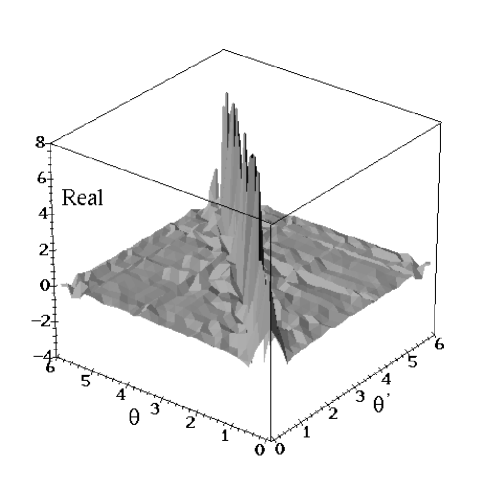
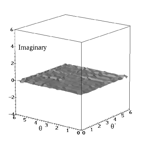
FIG. 2.: Presentation of the almost closure relation: $\sum_{l=1}^{Ne}\Psi_{l}^{*}(\theta^{\prime})\Psi_{l}(\theta)\sim\delta(\theta^{\prime}-\theta)$, see eqs.(14) and (15), for one ring of the disordered ensemble at convergence of the self consistency ($N_{s}=30$ random scatterers, $\Lambda=14$, $Ne=42$ electrons). The real part of the sum is concentrated at $\theta\sim\theta^{\prime}$. The imaginary part of the sum is vanishingly small. This figure justifies the approximation of the HF integro differential eq.(14) by eq.(15) that we self consistently solved. Note that the electronic wave functions $\Psi_{l}(\theta)$ are $2\pi$ periodic for any flux and so is the effective potential.

Here $V_{eff}(\theta)\psi(\theta)$ contains the three terms in the square brackets of eq.(14) with the approximated Fock term. The result of $\sum_{l=1}^{Ne}\Psi_{l}^{*}(\theta^{\prime})\Psi_{l}(\theta)$ for a typical realization is presented in Fig.2. It is clearly seen that, due to the sharpness of the almost closure relation, approximating eq.(14) by eq.(15) is reasonable. The approximation is reasonable for all electrons. At low energies the wave length of the considered electron is much larger than the width ${1\over N_{e}}\sim\lambda_{F}$ (where $\lambda_{F}$ is the Fermi wave length) and therefore the approximation is reasonable at low energies. For an electron near the Fermi energy $E>>V_{eff}(\theta)$ (where $V_{eff}(\theta)$ is defined to vanish at its minimum and is of the order of $\Lambda$) the error as a consequence of the approximation can not create any significant change in the current of such electron.

We solve eq.(15) self-consistently. For the n-th iteration the single electron wave functions from the previous iteration are taken and used to construct the effective potential $V_{eff}(\theta)$ for the current iteration. For the first iteration ($n=1$) we define $V_{eff}(\theta)$ by the non-interacting solutions, i.e., equivalent to setting $V_{eff}(\theta)\equiv 0$ at iteration $n=0$. The smooth $V_{eff}(\theta)$ is approximated by a constant potential in the intervals between the external impurities. If $N_{s}$ is small a finer subdivision of the intervals may be necessary. For the k-th interval $\theta_{k}\leq\theta<\theta_{k+1}$ the effective potential is defined as $V_{eff}(\theta)=V_{eff}(\theta_{k})$. The orthogonal solutions, which vary from one interval to the other, are given by $e^{\pm z_{k}\theta}$ where $z_{k}\equiv\sqrt{2(V_{eff}(\theta)-E)}$ is either real or pure imaginary. As one is free to add a global constant to the energy we define $V_{eff}(\theta)$ to be zero at its minimum. For that interval the general solution $\psi(\theta)$ is a linear combination of $\exp(\pm ix\theta)$ with some real positive $x$ that defines the energy $E=x^{2}/2$. Propagating $\psi(\theta)$ along the ring circumference[36], with an appropriate matching at the boundaries of all intervals, and applying the BC of eq.(4) yield the discrete spectrum [37] and eigen functions of eq.(15) which can now be normalized.

We shall now discuss the choice of parameters for the numerical solution of Eq.(15). The number of electrons in a given realization of disorder was set by requiring that the energy of the highest occupied state $l$ will be smaller than $312.5$, i.e., $x_{l}<25$, for any value of flux. This results in an average filling of $42$ electrons per realization. This requirement was chosen in order to balance between computation time limitations and maintaining enough electrons for the validity of the almost closure relation. This choice allows the study of different energy regimes such as the almost ballistic (higher energies), moderate (intermediate energies) and the strong (lower energies) disorder limit. The strength of the interaction term is determined by the ratio ${R\over r_{0}}$. For metals this ratio for a reasonable experimental setting (say $R=0.1\mu m$) will be about $10^{3}$, while for semiconductors (which have small effective masses and large dielectric constants) the ratio is of order of one. Since we can treat only a limited number of electrons, we are really considering the low density limit of the problem, which corresponds better to the semiconductor case and therefore we chose ${R\over r_{0}}=1$. A comparison between the TB model parameters and our estimation of the strength of interaction in semiconducting rings can be achieved by recognizing that for the typical densities of semiconducting devices the ratio of the electrostatic interaction energy $U$ to the kineic energy $t$ (the hopping matrix element) is of order of unity[semicond] for semiconductor. The cutoff was chosen as $\epsilon=10^{-5}$. It was checked that enlarging the cutoff up to $10^{-3}$ does not change the results within the limits of accuracy. As a convergence condition for the $n$-th iteration at a given flux we required: $\sum_{l=1}^{Ne}\mid x_{l}^{(n)}-x_{l}^{(n-1)}\mid<0.00025$. For a typical realization this condition was fulfilled within ten iterations.

In order to calculate the PC one can use two different approaches. The first is the derivative of the many particle ground state energy as function of the flux and the second is a direct application of the current operator on the many particle wave function. As we have confirmed both methods should give the same current, i.e.,

$$I_{v}=-c{\partial\over\partial\phi}<\Psi_{v}|{\bf H}|\Psi_{v}>=<\Psi_{v}|{\bf\hat{J}}|\Psi_{v}>.$$ (16)

Here, $I_{v}$ and $\Psi_{v}$ are the H-F ground PC and H-F ground state, ${\bf H}$ is the exact Hamiltonian. In the calculation of the current it is sometimes convenient to use the following relation[38]

$$\begin{array}[]{c}-c{\partial\over\partial\phi}<\Psi_{v}|{\bf H}|\Psi_{v}>\\ =-c\sum_{l=1}^{N_{e}}\left[{\partial\over\partial\phi}E_{l}-<\psi_{l}|\left({\partial\over\partial\phi}{\bf V}_{eff}\right)|\psi_{l}>\right]\end{array}$$ (17)

where $E_{l}$ are the eigenvalues of eq.(15). It is worthwhile to note that in the H-F approximation the PC is not simply the derivative of the sum of the H-F single particle eigenvalues $E_{l}$. The single level current for a particular level is defined as $i_{l}=-c\left[{\partial\over\partial\phi}E_{l}-<\psi_{l}|\left({\partial\over\partial\phi}{\bf V}_{eff}\right)|\psi_{l}>\right]$. We shall note that the PC and the eigen states of a clean ring are completely unaffected by the e-e interaction.

III Numerical results

In this section we shall describe the results of our self consistent numerical solution of Eq. (15). We have considered realizations with $N_{s}=30$ randomly placed delta scatterers of strength $\Lambda=14$ (see eq.(6)) for all the numerical calculations. The number of electrons occupying a specific realization was defined by the noninteracting problem as was explained in the previous sub-section. For a typical realization $N_{e}$ was of order of $42\pm 6$. $V_{eff}(\theta)$ was calculated as a staircase potential at $2N_{s}$ points (see the previous section for details) and was found to be a reasonable approximation of the smooth effective potential. Our ensemble of disordered rings contained 150 different realizations. In the following we present the results of our study of the effect of the e-e interactions on (A) the level spacing, (B) the PC distributions, and (C) the canonical average and the single ring PC.

A Spectrum

As mentioned in the introduction, one of the main advantages of the H-F approximation is that although one is dealing with a many particle problem the single electron levels still characterize the system. Thus, the immediate question arises whether e-e interactions imposes a transition on the level statistics. Because in the H-F approximation the system is still characterized by a single electron spectrum of an effective Hamiltonian (see eq.(15)), we were trying to answer this question by comparing the level spacing statistics of the eigenvalues of eq.(3) with that of eq.(15) when the condition for self consistency is satisfied. The level spacing statistics are considered for different regimes of disorder: (i) the extended regime (levels within a high energy strip) which corresponds to Wigner statistics for the noninteracting electrons; (ii) the localized regime (levels within a low energy strip) corresponding to the Poisson statistics for the noninteracting electrons. For these low energies the levels are clearly localized because the calculated levels currents were found to be exponentially small and by drawing $|\psi_{l}(\theta)|^{2}$ we simply visualized the localization. Fig.3 shows the results for both regimes. There is no transition in the level spacing due to the e-e interactions.

FIG. 3.: Comparison of level spacing statistics $P(s)$ of noninteracting (empty symbols) and interacting (bold symbols) electrons within the H-F approximation. (a) At high energy strip $P(s)$ is Wigner-Dyson $N(\beta)s^{\beta}\exp(a_{\beta}s^{2})$. $\beta=1,\;a_{1}=\pi/4,\;N(1)=\pi/2$ for zero flux (dashed), $\beta=2,\;a_{2}=4/\pi\;N(2)=32/\pi)$ for half quantum of flux (long-dashed). (b) At low energy strip the states are localized also when including interaction as can be seen from the statistics which remains Poissonian. Because the change from (a) to (b) is continuous as a function of energy and $P(s)$ is unchanged when including interaction there is no sign of interaction induced insulator to metal transition.

The same analysis was carried out for an intermediate regime (levels in a regime between (i) and (ii)) also did not show any difference between the statistics of the interacting and noninteracting electrons, although in both of these cases the expected transition from Poisson to Wigner statistics as a function of energy was found. Thus, the level statistics do not show any sign of an insulator to metal transition, which may be expected if the interactions induce a straight forward change in the localization properties of the H-F levels. Therefore, if there would be any enhancement of the PC (of this spinless model) it can not be explained by an interaction induced insulator to metal transition.

B Distributions of PC

FIG. 4.: Probabilities of sample PC for interacting (bold symbols) and noninteracting (empty symbols) electrons in the same canonical ensemble of 150 disordered rings at ${\phi\over\phi_{0}}=0.225$.

In order to understand the effect of e-e interactions on the canonical PC we plot the distribution of the canonical persistent currents for an ensemble of realizations with non-interacting electron as well as for the same realizations when interactions are taken into account. As can be clearly seen in Fig.4 the distribution of sample current is shifted towards more negative values, i.e. the PC becomes diamagnetic. Nevertheless, as a result of the interactions, individual realizations can change the current size and current direction in both the paramagnetic and diamagnetic directions. Unfortunately, because our ensemble is small it is meaningless to define the enhancement factor of the typical $\sqrt{\langle I^{2}\rangle}$ PC since it is strongly controlled by rare events in the tails. This shift of the distribution is similar to the situation seen in an exact diagonalization study of small 2D systems in the diffusive regime [20], although the direction is opposite[27].

FIG. 5.: Probabilities for level PC of interacting (bold symbols) and noninteracting (empty symbols) electrons in the same canonical ensemble of 150 disordered rings at ${\phi\over\phi_{0}}=0.225$. (a) For extended levels within two high energy strips. At the highest strip the states are close to ballistic and have greater probability to carry large positive or negative current. At the lower strip the probability is compared with a Gaussian (average and variance from numerical data) as predicted by Simons and Altshuler. Note the interaction induced diamagnetic levels currents. (b) For localized levels within two low energy strips. Note the horizontal logarithmic scale and the further suppression of PC due to interaction. (The visual shift between the distributions depends on the width of the horizontal bins).

To get an information on the single electronic levels we have also compared the probability distributions of the single level PC for noninteracting and interacting electrons. One should separately analyze the different regimes of disorder previously defined. In Fig.5a the distributions of single level PC are given for two different high energy strips in the extended regime. It is evident that due to the interaction the single level PCs are slightly shifted toward more negative values of the currents. The dip at the center of the probability distribution of the levels belonging to the highest energy strip is due to the fact that the electrons are almost ballistic and have a greater probability to carry large positive or negative current. In the lower energy strip the distribution follows a Gaussian shape as was found by Simons and Altshuler[39] for levels in the diffusive regime. In contrast to the high energy regime the effect of the interactions on electrons in the localized regime is to suppress the PC. This is clearly seen in Fig.5b where we considered levels belonging to two different low energy strips for which the electrons were found to be localized. Such suppression of the PC in the localized regime by e-e interactions was previously seen in H-F calculations of TB models[23], and in exact diagonalization of short range interacting electrons[19]. But exact diagonalization studies of TB models with long range interaction show enhancement in this regime[18]. We shall return to the origin of this discrepancy later on.

Because the total PC in a sample is dominated by electrons at high levels which have the largest current magnitude the canonical distribution of the sample PC, presented in Fig.4, is clearly dominated by the single level distribution presented in Fig5a. The asymmetry in the PC direction was also analyzed in the extended regime in terms of the distribution of levels curvatures $k\equiv-{\partial i_{l}\over\partial(\phi/\phi_{0})}$. Here the calculations were performed by applying the current operator on wave functions because in this method one can easily calculate the levels PCs at flux values close to zero or to half flux quantum which, for these flux values, are proportional to the curvatures[17]. The distributions of the curvatures were of course similar to the appropriate distributions in Fig5a.

C Canonical average and enhancement of the single ring PC

In the previous sub-sections we have presented data on the distribution of the canonical sample PC, single level PC and single level curvatures. We have seen a gradual shift in all of these distributions as a consequence of the e-e interactions. The sum over all electronic contributions from all samples gives the total current, and divided by the number of samples the average current. The average current as a function of flux is presented in Fig.6. Though the diamagnetic shift is clearly seen, the current amplitude is quite unchanged. This is very different than the suppression found in the various studies of 1D TB models in the weakly disordered regime [18, 19, 23]. Nevertheless, this does not present the whole picture. For a particular sample a strong suppression or enhancement of the PC amplitude due to the e-e interactions is possible. For example, a particular realization shown in Fig.7 demonstrates the highest effect of interaction on the PC of a single isolated ring that we found in our ensemble. The enhancement factor in this particular case is about $17$. Of course, even for this case, the current can not reach its clean ring value.

FIG. 6.: Comparison of the canonical average persistent current of interacting and noninteracting electrons in an ensemble of 150 disordered rings. The interaction effect is to shift the noninteracting curve towards more negative current values when the flux is positive. The $\phi_{0}/2$ periodicity is retained. However it is clear that the amplitude of the average current is not enhanced.

FIG. 7.: The highest enhancement factor ($\sim 17$) of single ring PC due to the interaction that was found among our ensemble. The ring contains 42 electrons. The resulting PCs while calculating $V_{eff}(\theta)$ at 60 and 90 points are compared. This figure demonstrates the possibility of a huge PC enhancement found in the single ring experiment.

IV conclusions

Our results within the self consistent HF approximation for the PC carried by spinless electrons in 1D disordered continuous rings with long range e-e interactions can be summarized as follows: The PC of states in the diffusive and ballistic regimes are not suppressed by the e-e interactions. This is in contrast to the suppression of the PC found in Refs. [18, 19] and [23] for the analogous TB models in these regimes of disorder. We found that the PC amplitude for the specific samples may be altered, but not the amplitude of the average or typical current current. Further, the distribution of the PC’s acquires a diamagnetic shift. This was confirmed by comparing the distributions of the individual levels currents, and also of the total currents, for noninteracting and interacting electrons. Because the total current of a sample is dominated by the extended states the average current per sample also shows a clear diamagnetic behavior. Our results are significantly different from those of TB models where the Mott-Hubbard transition was shown to plays a crucial role in suppressing the PC. In the continuous model the Mott-Hubbard transition does not show such a significant role. The concept of band and filling factor does not seem to be relevant. In the localized regime we found that the PC is further suppressed by the e-e interactions. This is an artifact of the H-F approximation which does not describe the appearance of density correlations in this regime. An exact diagonalization of small 1D TB rings with long-range interaction show that the PC is actually enhanced in this regime [18]. By studying the effect of e-e interaction on the level spacing statistics it is possible to gain a better understanding of the behavior of the current. The level spacing statistics show no sign of insulator to metal transition and this is consistent with the distributions found for the levels PC’s.

Introducing spin is expected to allow a stronger enhancement of the average current amplitude because of the fact that for spinless electrons the direct term is almost equal the absolute value of the exchange term, while when including the spin degree of freedom the direct term is about twice larger. This is crucial [17] for counteracting the disorder potential which leads to a higher PC amplitude. This explains the important role of spin for the enhancement of the PC as observed for 2D TB rings[26] when compared to the spinless case[24]. As we have seen in the 1D case the interactions are effective in changing the current in the regime of weak-disorder. One would expect the interaction to play an important role in the diffusive regime. In 1D systems the states are either localized or ballistic and therefore, the PC of the states are not strongly affected by the interactions. On the other hand, for higher dimensions where a true diffusive regime exists, one might expect for a stronger enhancement.

We conclude that the effect of e-e interactions in favor of the enhancement of the PC in a continuous disordered model is stronger than in TB models. This should be better revealed when one considers spin and higher dimensionality. We have shown that even for interacting spinless electrons in 1D no further suppression of the PC due to interaction occurs. This is in contrast to the further suppression of the current in the weakly disordered TB rings that was found in Refs.[18, 19] and[23].

REFERENCES

- [1] M. Büttiker, Y. Imry and R. Landauer, Phys. Lett. 96 A, 365 (1983)
- [2] N. Byers and C.N. Yang, Phys. Rev. Lett. 7, 46 (1961).
- [3] J. M. Blatt, Theory of superconductivity, pp. 307-344, Academic Press (1964).
- [4] Y. Imry, in Directions in condensed matter physics Eds. G. Grinstein and G. Mazenko, world scientific 1986.
- [5] H.F. Cheung, Y. Gefen, E.K. Riedel and W.H. Shih, Phys. Rev. B 37, 6050 (1988); H.F. Cheung, Y. Gefen and E.K. Riedel, IBM J. Res. Dev. 32, 358 (1988); H.F. Cheung, E.K. Riedel and Y. Gefen, Phys. Rev. Lett. 62, 587 (1989).
- [6] H. Bouchiat and G. Montambaux, J. Phys. (France), 50, 2695 (1989).
- [7] G. Montambaux, H. Bouchiat, D Sigeti, and R. Frisner, Phys. Rev. B 62, 587 (1989).
- [8] E. Akkermans and J. Montambaux, Phys. Rev. Lett. 68, 642 (1992); P. Schmitteckert and U. Eckern, cond-mat/9604005; G. Montambaux, J. Phys. I France 6, 1 (1996); D. Shepelyansky, Phys. Rev. Lett. 73, 2067 (1994); Y. Imry, Euro. Phys. Lett. 30, 405 (1995); D. Weinmann and J. L. Pichard, cond-mat 9602004. Y. V. Fyodorov, H.J. Sommers, Z. Phys. B 99, 123 (1995); J. Zakrzewski D. Delande, Phys. Rev. E. 47, 1650 (1993); A. Kamenev and D. Braun, J. Phys. I France 4, 1049 (1994).
- [9] D. Schmeltzer, Phys. Rev. B 47, 7591 (1993);
- [10] L.P. Levy, G. Dolan, J. Dunsmuir and H. Bouchiat, Phys. Rev. Lett. 64, 2074 (1990).
- [11] V. Chandrasekhar. R. A. Webb, M.J. Brady, M.B. Ketchen, W. J. Gallagher and A. Kleinsasser, Phys. Rev. Lett. 67, 3578 (1991).
- [12] D. Mailly, C. Chapelier and A. Benoit, Phys. Rev. Lett. 70 2020 (1993).
- [13] R. Berkovits and B. L. Altshuler, Phys. Rev. B 46, 12526 (1992).
- [14] U. Sivan, Y. Imry and A. Aronov Europhys. Lett. 28, 115 (1994).
- [15] For recent reviews on the metal-insulator transition see: D. Belitz and T.R. Kirkpatric, Rev. Mod. Phys. 66, 261 (1994); A. Geoges, G. Kotliar, W. Krauth and M. J. Rozenberg, Rev. Mod. Phys. 68, 13 (1996).
- [16] V. Ambegaokar and U. Eckern, Phys. Rev. Lett. 65, 381 (1990); A. Schmid, Phys. Rev. Lett. 66, 80 (1991); R.A. Smith and V. Ambegaokar, Europhys. Lett. 20, 161 (1992).
- [17] T. Giamarchi and B. Shastry, Phys. Rev. B 51, 10915 (1995).
- [18] M. Abraham and R. Berkovits, Phys. Rev. Lett. 70, 1509 (1993); Physica A 200, 519 (1993); R. Berkovits, Phys. Rev. B 48, 14381 (1993).
- [19] G. Bouzerar, D. Poilblanc and G. Montambaux, Phys. Rev.B. 49, 8258 (1994).
- [20] R. Berkovits and Y. Avishai, Europhys. Lett. 29, 475 (1995); Solid State Commun. 93, 301 (1995); Phys. Rev. Lett. 76, 291 (1996).
- [21] E.H. Lieb and F.Y. Wu, Phys. Rev. Lett. 20, 1445 (1968);
- [22] M. L. Mehta, Random matrices (Academic Press, San-Diego, 1991); L. P. Gorkov and G. M. Eliashberg, Zh. Eksp. Teor. Fiz. 48, 1407 (1965) [Sov. Phys. JETP 21, 940 (1965)]; B. L. Altshuler and B. I. Shklovskii, Zh. Eksp. & Teor. Fiz. 91, 220 (1986) [Sov. Phys. JETP 64,127 (1986)]; U. Sivan and Y. Imry, Phys. Rev. B 35, 6074 (1987).
- [23] H. Kato and D. Yoshioka, Phys. Rev. B 50, 4943 (1994).
- [24] G. Bouzerar and D. Poilblanc, Phys. Rev. B 52, 10772 (1995).
- [25] H. Kato and Y. Yoshioka, Physica B 212, 251 (1995).
- [26] G. Bouzerar and D. Poilblanc, cond-mat 9512153.
- [27] M. Ramin, B. Reulet, and H. Bouchiat, Phys. Rev. B 51, 5582 (1995).
- [28] M. Kamal, Z. H. Musslimani and, A. Auerbach, J. Phys. France 5, 1487 (1995).
- [29] A. Müller Groeling, H. A. Weidenmüller, and C. H. Lewnkopf, Europhys. Lett. 22, 193 (1993); H. A. Weidenmüller, Physica A 200, 104 (1993). A. Müller Groeling, H. A. Weidenmüller, Phys. Rev. B. 49, 4752 (1994).
- [30] Y. Imry and N.S. Shiren, Phys.Rev.B, 33, 7992 (1986).
- [31] E. Abrahams, P. W. Anderson, D. C. Licciardello, and T. V. Ramakrishnan, Phys. Rev. Lett. 42, 673 (1979); E. Abrahams, P. W. Anderson, and T. V. Ramakrishnan, Phil. Mag. B42, 827 (1980). A. Cohen, Y. Roth and B.Shapiro Phys. Rev. B 38, 12125 (1988); A. Cohen and B. Shapiro Int. J. Mod. Phys. B 6, 1243 (1992); B.L. Al’tshuler, V.E. Kravtsov, and I. Lerner in Mesoscopic Phenomena in Solids, edited by B.L. Al’tshuler, P.A. Lee, and R.A. Webb (North Holland, Amsterdam, 1991).
- [32] The fluctuations flows with towards a universal lognormal distribution characterized by only two parameters: the average and variance of both grow linearly with . The microscopic values at are dictated by the nonuniversal microscopic fluctuations, i.e. the microscopic disorder.
- [33] P. W. Anderson and P. A. Lee, Prog. Theor. Phys. Suppl. (Japan) 69, 212 (1980). Concerning the eigenvalues see A. Cohen Phys. Rev. B. 51, 10406 (1995).
- [34] B. L. Altshuler, Y. Imry and Y. Gefen, Phys. Rev. Lett. 66, 88 (1991).
- [35] Rubin H. Landau in Quantum mechanics II, p.194 (John Wiley & sons, 1990).
- [36] At this point we defined the origin at the left point of the (sub)interval where . Note also that only when completing a propagation of the solution around the ring one has in hand a transfer matrix. The spectrum and eigen functions are independent of the shift of the origin.
- [37] We searched for zeroes (as a function of wave vector ) of the difference between the real part of the eigen values of (the transfer matrix for full circumference) and the desired phase value . We divided the wave vector axis to tiny intervals in which whenever a sign change occurred in a numerical zero with accuracy of was searched. defines the minimum level spacing we are always able to detect.
- [38] E. Merzbacher in Quantum mechanics; 2ed edition; J. Wiley Sons (1970).
- [39] B. D. Simons and B. L. Altshuler, Phys. Rev. B. 48, 5422 (1993).