AN INVESTIGATION OF THE 2D ATTRACTIVE HUBBARD MODEL
R. Lacaze^ab, A. Morel^a, B. Petersson^c and J. Schröper^c

^a Service de Physique Théorique, CEA-Saclay, 91191 Gif-sur-Yvette Cedex, France

^bASCI, Bat. 506, Université Paris Sud, 91405 Orsay Cedex, France

^c Fakultät für Physik, Universität Bielefeld, Postfach 10 01 31, D-33501 Bielefeld, Germany

Abstract

We present an investigation of the 2D attractive Hubbard model, considered as an effective model relevant to superconductivity in strongly interacting electron systems. We use both hybrid Monte Carlo simulations and existing hopping parameter expansions to explore the low temperature domain. The increase of the static S-wave pair correlation with decreasing temperature is analyzed in terms of an expected Kosterlitz-Thouless superconducting transition. The evidence for this transition is weak: If it exists, its temperature is very low and depends weakly on the band filling near half filling. The number of unpaired electrons remains nearly constant with temperature at fixed attractive potential strength. In contrast, the static magnetic susceptibility decreases fast with temperature, and cannot be related only to pair formation. We introduce a method by which the Padé approximants of the existing series for the susceptibility give sensible results down to rather low temperature region, as shown by comparison with our numerical data. PACS 71.10.Fd 74.25.Dw 75.40.Mg

October 1996                  Submitted for publication to J. Phys. I (France)

BI-TP 96/05
T96/ 114

1. Introduction

The study of models of strongly interacting electrons is very important for the understanding of high temperature superconductivity. The fundamental mechanism of this phenomenon has not yet been clearly identified, and it may be interesting to study effective models, which have strong local attraction between the electrons. The two dimensional attractive Hubbard [1] model is an example of such a model whose phase diagram as well as physical properties in the normal non superconducting phase can be compared to properties of actual superconducting materials of the high $T_{c}$ superconductivity class.

The two dimensional attractive Hubbard model is a conceptually simple model, which at low temperatures is expected to have a Kosterlitz-Thouless transition [2] into a superconducting phase, away from half filling. At half filling the model has further symmetries, which prevents such a transition. In the absence of magnetic field, the properties of the model depend on two parameters (apart from the temperature) namely the coupling constant of the attractive local interaction $U$ and the chemical potential $\mu$, measured in units of the coefficient $k$ of the hopping term. The model is solvable in the free case $U=0$ and the atomic limit $k=0$. In the interesting case where both $U$ and $k$ are different from zero the model can only be studied through developments around the two solvable cases, high temperature series and numerical simulation techniques. In contrast to the repulsive Hubbard model, with the opposite sign of U, the fermionic determinant is positive also for chemical potential different from zero. Thus the numerical simulations do not suffer from the sign problem in this case. In fact, the two models are related by a change of sign in $U$ and the exchange of chemical potential and magnetic field.

In this paper, using a hybrid Monte Carlo algorithm, we perform a detailed numerical study of the model in a wide range of values of the parameters. The purpose is first to examine in detail the evidence for a Kosterlitz-Thouless transition and, if it takes place, to estimate the critical temperature. This can be done by studying the s-wave pair-field correlation function, which should diverge at the transition on an infinite lattice. Another interesting quantity is the magnetic susceptibility, sensitive to the presence of single electrons as contrast to those bound in pairs. One may expect the susceptibility to disappear in the strong coupling limit, where more and more pairs are formed. However, at fixed $U$ the temperature behavior of the probability that a site has a single electron and the behavior of the susceptibility are not the same. Therefore the behavior in temperature of the susceptibility of the remnant unpaired electrons is interesting to investigate. For this latter quantity we make use of the series expansion in $k$ given in Ref.[3], and with the help of the Padé approximants method, extrapolate the series to low temperatures. We compare the results with our numerical data and show that, at least at small and intermediate couplings, rather low temperature may be reached analytically. If true also in the repulsive case of the Hubbard model, where numerical simulations suffer from the sign problem, series expansion might be interesting to use. Unfortunately, no such series are available for the pair field correlator.

There have been some earlier numerical investigations of this model [4, 5], leading in particular to estimates of the transition temperature. We compare our estimates to theirs, when there is overlap in the parameters. Our estimate of the transition temperature is considerably lower than in these investigations. In particular, for the range of temperatures we simulated, we do not see a really significant difference between the half filled case, where no transition is expected, and away from half-filling.

In Section 2 we define the model and the observables, which we measure. Section 3 is devoted to the formulation of the path integral formalism needed for the numerical simulation. In Section 4 we discuss the algorithm employed, which we have chosen as the Hybrid Monte Carlo algorithm. In Section 5 we discuss our data on the pair field correlation, which is a direct indicator of a transition into a superconducting phase. In Section 6 we present results for the susceptibility, comparing our numerical results with analytic results extrapolated from the series expansion. Section 7, finally, contains a summary and our conclusions.

2. The Model

The model is defined by the Hubbard Hamiltonian

$$H = -k\sum_{\left<x,y\right>}\left(a^{\dagger}_{x}a_{y}+a^{\dagger}_{y}a_{x}+b^{\dagger}_{x}b_{y}+b^{\dagger}_{y}b_{x}\right)-U\sum_{x}\left(a^{\dagger}_{x}a_{x}-\frac{1}{2}\right)\left(b^{\dagger}_{x}b_{x}-\frac{1}{2}\right)$$ (1)

$$-\mu\sum_{x}\left(a^{\dagger}_{x}a_{x}+b^{\dagger}_{x}b_{x}\right)\hskip 12.0pt,$$

where x and y are sites on a two dimensional $N_{s}\times N_{s}$ square lattice with $V=N_{s}^{2}$ sites, $a_{x}$ and $b_{x}$ are coordinate space annihilation operators for spin-up and spin-down electrons respectively, and $k$ is the nearest neighbor hopping parameter. The coupling $U>0$ denotes the strength of the attractive local interaction and $\mu$ is the chemical potential, defined so that $\mu=0$ at half filling, i.e. where the total particle number $\left<N\right>=V$. Here

$$N=\sum_{x}(a^{\dagger}_{x}a_{x}+b^{\dagger}_{x}b_{x})\hskip 12.0pt.$$ (2)

We also define the particle number density operator

$$n=\frac{1}{V}N\hskip 12.0pt.$$ (3)

We do not couple the system to an external magnetic field. Thus the model is invariant under an $SU(2)_{\rm spin}$. For $\mu=0$ it is also invariant under another $SU(2)$ group [6], generated by the operators

$$J^{\prime}_{-} = \sum_{x}(-)^{x}a_{x}b_{x}\hskip 12.0pt,$$

$$J^{\prime}_{+} = J^{\prime\dagger}_{-}\hskip 12.0pt,$$

$$J^{\prime}_{0} = \frac{1}{2}\left(N-V\right)\hskip 12.0pt.$$ (4)

The thermodynamics of the model is given by the partition function

$$Z=\mbox{Tr}\left(e^{-\beta H}\right)\hskip 12.0pt.$$ (5)

In the simulation we will measure average values of operators in this ensemble,

$$\left<O\right>=\mbox{Tr}(Oe^{-\beta H})/Z\hskip 12.0pt.$$ (6)

The basic equal time correlation functions, which give information about the properties of the model are the S-wave on site pairing correlation function

$$P(x-y)=\left<(a^{\dagger}_{x}b^{\dagger}_{x}+b_{x}a_{x})(a^{\dagger}_{y}\ b^{\dagger}_{y}+b_{y}a_{y})\right>\hskip 12.0pt,$$ (7)

the magnetization density correlation function, or magnetic susceptibility

$$\chi(x-y)=\beta\left<(a^{\dagger}_{x}a_{x}-b^{\dagger}_{x}b_{x})(a^{\dagger}_{y}a_{y}-b^{\dagger}_{y}b_{y})\right>\hskip 12.0pt,$$ (8)

and the charge density correlation function

$$C(x-y)=\left<(a^{\dagger}_{x}a_{x}+b^{\dagger}_{x}b_{x})(a^{\dagger}_{y}a_{y}+b^{\dagger}_{y}b_{y})\right>\hskip 12.0pt.$$ (9)

The probability that a site is singly occupied is

$$S_{1}=\frac{\chi(0)}{\beta}\hskip 12.0pt.$$ (10)

Furthermore

$$P(0)=1-S_{1}\hskip 12.0pt$$ (11)

is the probability of zero or double occupancy.

The correlation function in Fourier space of the quantity $E$ denoted by $\widetilde{E}$ is defined as

$$\widetilde{E}(q)=\sum_{z}e^{iqz}E(z)\hskip 12.0pt.$$ (12)

An indicator of the diverging correlation length at the phase transition, which has been used e.g. in [4, 5] is

$$\widetilde{P}_{0}\equiv\widetilde{P}\left(q=(0,0)\right)\hskip 12.0pt.$$ (13)

In the same way, the charge density wave indicator is $\widetilde{C}(\pi,\pi)$ and the uniform spin susceptibility is given by $\widetilde{\chi}(0,0)$.

From the $SU(2)^{\prime}$ symmetry, it follows that at $\mu=0$ the Hamiltonian is invariant in particular under the transformation

$$(a_{x},b_{x})\to(\alpha_{x},\beta_{x})$$ (14)

with

$$a_{x}=\frac{1}{\sqrt{2}}\left(\alpha_{x}+\beta_{x}^{\dagger}(-)^{x}\right)\hskip 12.0pt,$$ (15)

$$b_{x}=\frac{1}{\sqrt{2}}\left(\beta_{x}-\alpha_{x}^{\dagger}(-)^{x}\right)\hskip 12.0pt.$$ (16)

Using that $\mu=0$ implies half filling, i.e. $\left<n\right>=1$, this leads to

$$P(z)=(-)^{z}\left[C(z)-1\right]\hskip 12.0pt.$$ (17)

The model is soluble in the two limiting cases $U=0$ (the free case) and $k=0$ (the atomic limit). For reference, these solutions and the corresponding values of the correlation functions are given in Appendix A.

3. The Path Integral Formulation

For the numerical simulation we use the path integral formalism, as described in Ref. [7]. We begin with the Trotter break-up

$$e^{-\beta H}=\left(e^{-\frac{\beta H}{N_{t}}}\right)^{N_{t}}$$ (18)

and label each of the $N_{t}$ factors by an imaginary time index $t$ running from 1 to $N_{t}$. One can then split the hopping term from the interaction term

$$e^{-\frac{\beta H}{N_{t}}} = \exp\left[\frac{k\beta}{N_{t}}\sum_{\left<x,y\right>}\left(a^{\dagger}_{x}a_{y}+a^{\dagger}_{y}a_{x}+b^{\dagger}_{x}b_{y}+b^{\dagger}_{y}b_{x}\right)\right]$$ (19)

$$\times\exp\left[\frac{U\beta}{N_{t}}\sum_{x}\left(a^{\dagger}_{x}a_{x}-\frac{1}{2}\right)\left(b^{\dagger}_{x}b_{x}-\frac{1}{2}\right)+\frac{\mu\beta}{N_{t}}N\right]\hskip 6.0pt,$$

making an error of order $\frac{kU\beta^{2}}{N_{t}^{2}}$. As a next step we introduce a scalar field $\left\{\sigma_{x,t}\right\}$ for the time slice $t$ in order to eliminate the four fermion term

$$e^{-\frac{\beta H}{N_{t}}} = \frac{1}{\left({2\pi}\right)^{V/2}}\int\prod_{x}\left[\mbox{d}\sigma_{x,t}\right]e^{-\frac{1}{2}\sum_{x}\sigma_{x,t}^{2}}\exp\Bigg{[}\frac{k\beta}{N_{t}}\sum_{\left<x,y\right>}\left(a^{\dagger}_{x}a_{y}+a^{\dagger}_{y}a_{x}\right)$$ (20)

$$+\frac{k\beta}{N_{t}}\sum_{\left<x,y\right>}\left(b^{\dagger}_{x}b_{y}+b^{\dagger}_{y}b_{x}\right)$$

$$+\sum_{x}\left(a^{\dagger}_{x}a_{x}+b^{\dagger}_{x}b_{x}\right)\left\{\sqrt{\frac{U\beta}{N_{t}}}\sigma_{x,t}+\left(\mu-U\right)\frac{\beta}{N_{t}}\right\}\Bigg{]}\hskip 12.0pt.$$

Furthermore, we use the two relations

$$\exp\left[a_{x}^{\dagger}a_{y}\right]=1+a_{x}^{\dagger}a_{y},x\neq y\;\;\mbox{ and }\;\;\exp\left[\alpha a_{x}^{\dagger}a_{x}\right]=1+a_{x}^{\dagger}a_{x}\left[e^{\alpha}-1\right]\hskip 12.0pt,$$ (21)

and the same relations for $b^{\dagger}$ and $b$ to transform the sums in the exponential of Eq. (20)

$$\exp\left[\frac{k\beta}{N_{t}}\sum_{\left<x,y\right>}\left(a^{\dagger}_{x}a_{y}\right)\right]=\prod_{\left<x,y\right>}\left(1+\frac{k\beta}{N_{t}}a^{\dagger}_{x}a_{y}\right)+O\left(\frac{k\beta}{N_{t}}\right)^{2}$$ (22)

and

$$\exp\left[\sum_{x}a^{\dagger}_{x}a_{x}\left(\sqrt{\frac{U\beta}{N_{t}}}\sigma_{x,t}+{\rm const.}\right)\right]=\qquad\qquad\qquad$$

$$\prod_{x}\left(1+a^{\dagger}_{x}a_{x}\left(\exp\left[\sqrt{\frac{U\beta}{N_{t}}}\sigma_{x,t}+{\rm const.}\right]-1\right)\right) \hskip 12.0pt.$$ (23)

For every time slice we put the appropriate factors together and use the anticommutation relations to transform the expression into a sum of normal ordered operators, neglecting terms of higher order in $1/N_{t}$. The trace of the product of normal ordered expressions in the fermion operators can be transformed into Grassmann integrals in the standard fashion [7], using

$$\mbox{Tr}\left[\prod_{i=1}^{N_{t}}:f_{i}\left(a^{\dagger},a\right):\right]=\int\prod_{t=1}^{N_{t}}\left[\left(\mbox{d}\bar{\eta}_{t}\right)f_{t}\left(\bar{\eta}_{t},\eta_{t}\right)\left(\mbox{d}\eta_{t}\right)e^{\bar{\eta}_{t}\left(\eta_{t}-\eta_{t-1}\right)}\right]$$ (24)

with the boundary condition $\eta_{0}=-\eta_{N_{t}}$ and similarly for $f_{i}(b^{\dagger},b)$. Finally, we obtain the partition function $Z$, up to an unimportant numerical coefficient, as

$$Z = \int\prod_{x,t}\left[\mbox{d}\sigma_{x,t}\right]e^{-\frac{1}{2}\sum_{x,t}\sigma^{2}_{x,t}}\int\prod_{x,t}\left[\mbox{d}\eta_{x,t}\mbox{d}\bar{\eta}_{x,t}\right]\prod_{x,t}\left[\mbox{d}\theta_{x,t}\mbox{d}\bar{\theta}_{x,t}\right]$$ (25)

$$\ \exp\Bigg{[}\frac{k\beta}{N_{t}}\sum_{\left<x,y\right>,t}\left(\bar{\eta}_{x,t}\eta_{y,t}+\bar{\eta}_{y,t}\eta_{x,t}\right)$$

$$\qquad+\sum_{x,t}\bar{\eta}_{x,t}\left(\eta_{x,t}-\eta_{x,t-1}\right)$$

$$\qquad+\sum_{x,t}\bar{\eta}_{x,t}\eta_{x,t}\left(\mbox{exp}\left[\sqrt{\frac{U\beta}{N_{t}}}\sigma_{x,t}-(U-\mu)\frac{\beta}{N_{t}}\right]-1\right)$$

$$+ \ \ \left\{\eta\to\theta\right\}\Bigg{]}\hskip 12.0pt,$$

when the $\bar{\theta},\theta$ Grassmann variables are associated with $b^{\dagger},b$. This defines a fermionic matrix $M$, specified for each set of $\sigma$-fields by its elements between the vectors $\bar{\eta}_{y,t^{\prime}}$ and $\eta_{x,t}$

$$\bar{\eta}M\eta = \frac{k\beta}{N_{t}}\sum_{\left<x,y\right>,t}\left(\bar{\eta}_{x,t}\eta_{y,t}+\bar{\eta}_{y,t}\eta_{x,t}\right)-\sum_{x,t}\bar{\eta}_{x,t}\eta_{x,t-1}$$ (26)

$$+\sum_{x,t}\bar{\eta}_{x,t}\eta_{x,t}\mbox{exp}\left[\sqrt{\frac{U\beta}{N_{t}}}\sigma_{x,t}-(U-\mu)\frac{\beta}{N_{t}}\right]\hskip 12.0pt.$$

The integrals over the Grassmann variables may be performed, and we get

$$Z=\int\prod_{x,t}\left[\mbox{d}\sigma_{x,t}\right]e^{-\frac{1}{2}\sum_{x,t}\sigma^{2}_{x,t}}\left(\mbox{det}M\right)^{2}\hskip 12.0pt.$$ (27)

Furthermore $\mbox{det}M=\left(\mbox{det}M\right)^{\dagger}$, so that $\left(\mbox{det}M\right)^{2}=\mbox{det}\left(M^{\dagger}M\right)$, which is useful for the construction of the algorithm. It is possible to include the terms of order $1/N^{2}_{t}$ in the action. They are given in Appendix B and included in the simulation.

In order to compute expectation values of observables, it is convenient to first consider that of the operator

$$O\equiv\exp\left[-a^{\dagger}j\right]\exp\left[\bar{j}a\right]$$ (28)

when $\bar{j},j$ are Grassmann sources for the operators $a,a^{\dagger}$ taken at equal time, say $t=0$. Inserting $O$ as an additional factor into the l.h.s. of Eq. (24) corresponds to insert the factor $\widetilde{O}$ into its r.h.s., where

$$\widetilde{O} = \int\mbox{d}\eta_{N_{t}+1}\mbox{d}\bar{\eta}_{N_{t}+1}\exp\left[\bar{j}\eta_{N_{t}+1}+\bar{\eta}_{N_{t}+1}j\right]$$ (29)

$$\times \exp\left[\bar{\eta}_{N_{t}+1}\left(\eta_{N_{t}+1}-\eta_{N_{t}}\right)\right]$$

$$\times \exp\left[\bar{\eta}_{1}\left(\eta_{N_{t}+1}-\eta_{N_{t}}\right)\right]\hskip 12.0pt.$$

This is obtained by associating to $\left(a,a^{\dagger}\right)$ an additional Grassmann pair $\left(\eta_{N_{t}+1},\bar{\eta}_{N_{t}+1}\right)$, taking care of the boundary conditions which now says $\eta_{0}=-\eta_{N_{t}+1}$ instead of $\eta_{0}=-\eta_{N_{t}}$ (this explains the last exponential above). Explicit integration yields

$$\widetilde{O}=\exp\left[\bar{j}\eta_{N_{t}}+\bar{\eta}_{1}j+\bar{j}j\right]\hskip 12.0pt.$$ (30)

In fact $O$ could have been inserted in the trace between any two successive time slices $t$ and $t+1$ (with the same result for the trace due to cyclic invariance). The resulting $\widetilde{O}$ would then read

$$\widetilde{O}=\exp\left[\bar{j}\eta_{t}-\bar{\eta}_{t+1}j+\bar{j}j\right]\hskip 12.0pt.$$ (31)

This technique generalizes to the computation of any (time dependent) correlator $\zeta$. After $\zeta$ is rewritten in normal order (any creation operator brought to the left of any annihilation operator by repeated use of their commutation relations), one makes the replacement in $\zeta\left(\left\{a^{\dagger}\right\}\left\{a\right\}\right)$

$$\left\{a_{x}^{\dagger}\left[t\right],a_{y}\left[u\right]\right\}\to\left\{\frac{\partial}{\partial j^{\left(a\right)}_{x,t+1}},\frac{\partial}{\partial\bar{j}^{\left(a\right)}_{y,u}}\right\}\hskip 12.0pt,$$ (32)

the similar one for the $b$’s, and ends up with the final result:

$$\left<\zeta\right>=\zeta\left(\left\{\frac{\partial}{\partial j}\right\},\left\{\frac{\partial}{\partial\bar{j}}\right\}\right)\mbox{ln}Z\left(\bar{j},j\right)\Bigg{|}_{j=\bar{j}=0}\hskip 12.0pt,$$ (33)

where

$$Z\left(\bar{j},j\right)=\int \prod\limits_{x,t}\left[\mbox{d}\sigma_{x,t}\exp\left(-\frac{\sigma_{x,t}^{2}}{2}\right)\right]\times\left(\mbox{det}M\right)^{2}\times$$

$$\times \exp\left[\bar{j}^{\left(a\right)}M^{-1}j^{\left(a\right)}+\sum\limits_{x,t}\bar{j}_{x,t}^{\left(a\right)}j_{x,t+1}^{\left(a\right)}+a\leftrightarrow b\right]\hskip 12.0pt.$$ (34)

For the observables of interest, listed in Eqs. (3, 7 - 9), the following expressions then follow.

$$\left<n\right>=2-2\left<M^{-1}_{x,N_{t};x,1}\right>\hskip 12.0pt,$$ (35)

$$P(x-y)=\delta_{xy}\left[1-2\left<M^{-1}_{x,N_{t};x,1}\right>\right]+2\left<\left(M^{-1}_{x,N_{t};y,1}\right)^{2}\right>\hskip 12.0pt,$$ (36)

$${\chi(x-y)\over\beta}=2\delta_{xy}\left<M^{-1}_{x,N_{t};x,1}\right>-2\left<M^{-1}_{x,N_{t};y,1}M^{-1}_{y,N_{t};x,1}\right>\hskip 12.0pt,$$ (37)

$$C(x-y)= 2\delta_{xy}\left<M^{-1}_{x,N_{t};x,1}\right>+4-8\left<M^{-1}_{x,N_{t};x,1}\right>$$ (38)

$$+ 4\left<M^{-1}_{x,N_{t};x,1}M^{-1}_{y,N_{t};y,1}\right>-2\left<M^{-1}_{x,N_{t};y,1}M^{-1}_{y,N_{t};x,1}\right>\hskip 12.0pt.$$

We will also consider the average value of the field $\sigma_{x}^{\prime}$ defined as

$$\sigma_{x,t}^{\prime}=\sqrt{\frac{N_{t}}{\beta}}\sigma_{x,t}\hskip 12.0pt.$$ (39)

Indeed, from the equation of motion for the $\sigma$-fields, which can easily be derived from Eq. (20) or (25), we have

$$\lim\limits_{N_{t}\to\infty}\left<\sigma_{x,t}^{\prime}\right>=\sqrt{U}\left<n\right>\hskip 12.0pt.$$ (40)

This relation, together with $\left<n\right>=1$ at $\mu=0$ in the large $N_{t}$ limit (at finite $N_{t}$ the particle-hole symmetry is broken [7]), will be used as a check that we actually considered large enough $N_{t}$ values.

4. The numerical simulation

The expectation values of (35-39) are obtained from $\sigma$-field configurations corresponding to the partition function (27). These configurations are generated with an Hybrid Monte Carlo algorithm (HMC-algorithm) which is a widely used tool to simulate systems involving the fermion matrix (e.g. [7], [8], [9]). Its main virtues are that it is an exact algorithm and that, at least in principle, the computer time grows slowly with system size.

Introducing one set of pseudofermion fields $\phi^{(i)}$ for each species $\eta$ and $\theta$ and momenta $p$ conjugate to the $\sigma$ fields, the Hamiltonian of the system can be written as

$${\cal H}=\frac{1}{2}\sum\limits_{j}p_{j}^{2}+\frac{1}{2}\sum\limits_{j}\sigma_{j}^{2}+\sum_{i=1}^{2}\sum\limits_{j,k}{\phi_{j}^{(i)}}\left(M^{\dagger}M\right)_{jk}^{-1}\phi_{k}^{(i)}\hskip 12.0pt,$$ (41)

where $j$ and $k$ denote sites on the $N_{s}^{2}\times N_{t}$ lattice. Starting from a configuration $\sigma$, a new configuration is obtained in three steps.

• First the pseudofermion fields are generated from gaussian distributed vectors $r^{(i)}$ by $\phi^{(i)}=M^{\dagger}(\sigma)r^{(i)}$ and gaussian momenta $p$ are chosen.

• Then $\sigma$ and $p$ are updated by molecular dynamics with ${\cal H}$ as Hamiltonian, the set of Hamilton’s equations being solved with a discrete time step $\mbox{d}\tau$. So $\cal{H}$ is a constant of motion in the limit $\mbox{d}\tau\to 0$. The integration of the molecular dynamics equation is performed by a leapfrog method [8]

  $$\sigma_{j}|_{(n+1){\rm d}\tau} = \sigma_{j}|_{n{\rm d}\tau}+\mbox{d}\tau\ p_{j}-\frac{(\mbox{d}\tau)^{2}}{2}\left.\frac{\partial{\cal H}}{\partial\sigma_{j}}\right|_{n{\rm d}\tau}\hskip 12.0pt,$$ (42)

  $$p_{j}|_{(n+1){\rm d}\tau} = p_{j}|_{n{\rm d}\tau}-\frac{\mbox{d}\tau}{2}\left(\left.\frac{\partial{\cal H}}{\partial\sigma_{j}}\right|_{n{\rm d}\tau}+\left.\frac{\partial{\cal H}}{\partial\sigma_{j}}\right|_{(n+1){\rm d}\tau}\right)\hskip 12.0pt.$$ (43)

• After $n_{\rm MD}$ steps, the resulting $\sigma$ configuration is accepted or refused by a Metropolis test.

This algorithm introduces two parameters, the number of steps $n_{\rm MD}$ and the step size ${\rm d}\tau$. The correlation between configurations decreases when the trajectory length $\tau=n_{\rm MD}\mbox{d}\tau$ increases, while increasing $n_{\rm MD}$ increases the computation time and increasing $\mbox{d}\tau$ decreases the acceptance. We have taken $\tau\sim 1.0$, (more precisely between 0.8 and 1.6) with $n_{\rm MD}$ such that a large enough acceptance is reached for all the volumes used (the acceptance decreases with increasing volume [7],[8]). This is obtained with $n_{\rm MD}\sim 4\beta U$. We also tested trajectories with Poisson-distributed lengths, i.e. $n_{\rm MD}$ distributed around a certain mean value and $\mbox{d}\tau$ held fixed [10, 11]. This does not decorrelate measurements of observables compared to $\tau$ fixed. The only effect is to increase the acceptance a few percent if $n_{\rm MD}$ is small.

For an observable $O$ whose value at Monte Carlo time is $O_{i}$ the autocorrelation function is

$$C_{O}(t)=\frac{\left<O_{i}O_{i+t}\right>-\left<O_{i}\right>^{2}}{\left<O_{i}^{2}\right>-\left<O_{i}\right>^{2}}\hskip 12.0pt.$$ (44)

We estimated the autocorrelation time $\xi_{O}$ by

$$\xi_{O}=\frac{1}{t_{c}}\sum_{0}^{t_{c}-1}\ln\left[\frac{C_{O}(t+1)}{C_{O}(t)}\right]\hskip 12.0pt,$$ (45)

disregarding the noisy region $t>t_{c}$ where $C_{O}(t)$ is less than 0.05. This gives the exact autocorrelation time if $C_{O}$ is purely exponential. The integrated autocorrelation time

$$t_{\rm int}=\sum_{0}^{t_{c}-1}C_{O}(t)\hskip 12.0pt,$$ (46)

coincides with $\xi_{O}$ within 5% under the same assumption.

The physical and algorithmic parameters are given in Tables (1,2) along with the number of trajectories simulated, the autocorrelation time $\xi_{\sigma^{\prime}}$ and the acceptance. Other autocorrelation times connected to fermionic quantities are always very small as compared to $\xi_{\sigma^{\prime}}$. With the parameters chosen, the smallest values of the acceptance at $U=4$ are 0.64 for the lattice $8^{2}\times 64$ at $\beta=6$ and 0.71 for the lattice $8^{2}\times 32$ at $\beta=4$.

The updates of $\sigma_{j}$ and $p_{j}$ (Eqs. 42, 43) require twice the computation of a vector $u=\left(M^{\dagger}M\right)^{-1}\phi$ for a given $\phi$. This computation, which costs most of the computer time, is performed by a conjugate gradient subroutine with a diagonal preconditioning [12], which speeds up the convergence considerably. The conjugate gradient iteration is stopped after $c_{cg}$ steps, when $\left|\left(M^{\dagger}M\right)u_{c_{cg}}-\phi\right|^{2}$ becomes less than $10^{-10}$ times the value obtained for the initial guess $u_{0}$.

The number of conjugate-gradient iterations can be significantly reduced if we use for $u_{0}$ the value obtained at the previous molecular dynamics step. However this method leads to dramatic decreases of the acceptance when increasing $\beta$ and $V$. So we always start with $u_{0}=0$, in such a way that no peculiar direction of phase space is favored or suppressed by the numerical uncertainties.

The number of conjugate gradient iterations needed to reach the prescribed accuracy ranges between $\sim 30\%$ and $\sim 65\%$ of the vector length. However in some cases, this accuracy is not obtained in $N_{s}^{2}\times N_{t}$ iterations, in particular for small volumes. Such situations can be avoided by reducing the trajectory length $\tau$, and this explains the values $\tau=0.8$ and 1.2 in Table (1). However, this comes with the price of increasing the $\sigma$ autocorrelation times.

The matrix $M$ used in this computation is given in Eq. (Appendix B) of Appendix B. It is valid to order $1/N_{t}^{2}$. Some of the effects of using this second order matrix instead of the first order matrix of Eq. (26) are shown in Table (3). At $\mu=0$, and for $N_{t}$ large enough, one expects $\left<n\right>$ to approach 1 and, according to Eqs. (39,40), $\left<\sigma^{\prime}_{x,t}\right>$ to approach $\sqrt{U}$. This is clearly better achieved with the improved action (Appendix B). While $\widetilde{P}_{0}$ is not affected within errors by the change of the action, $\widetilde{\chi}$ unexpectedly happens to depend more on $N_{t}$ in the second order case.

Because increasing $N_{t}$ is costly in computer time, we currently used $N_{t}=2\beta U$. The exceptions, apart for analysis of $N_{t}$ dependencies, concern the case $\beta=0.5$, $U=8$ $(N_{t}=32)$ and the low temperature points $\beta=6$, $U=4$ $(N_{t}=64)$.

The results obtained for $\left<\sigma^{\prime}\right>$, filling of the band $\left<n\right>/2$, pairing correlation $\widetilde{P}_{0}$, spin susceptibility $\widetilde{\chi}$ and single occupation probability $S_{1}$ for various lattices and values of the inverse temperature $\beta$ and chemical potential $\mu$ are given in Tables (4,5). The errors reported therein are calculated by incorporating the autocorrelation time $t_{\rm int}$ of Eq. (46) by using a variance which is the naive variance multiplied by $(1+2t_{\rm int})$.

We cannot compare the efficiency of our algorithm with Quantum Monte Carlo [13], because for that algorithm we do not have the information needed.

5. The S-Wave Pair-Field Correlation Function

One of the observables of interest in the context of a superconducting phase transition is the pairing correlation function $P$ and its Fourier transform $\widetilde{P}$. They are defined by (7) and (12) respectively. In the present work we have studied the $q=(0,0)$ equal-time s-wave pair-field correlation function $\widetilde{P}_{0}$, Eq. (13), which has previously been examined e.g. in [4, 5]. For this quantity we obtain from Eq.(36)

$$\widetilde{P}_{0}=1-2\left<M^{-1}_{x,N_{t};x,1}\right>+2\sum\limits_{y}\left<\left(M^{-1}_{y,N_{t};x,1}\right)^{2}\right>\hskip 12.0pt.$$ (47)

Let us recall [4, 5] what can be expected on general grounds for the behavior of $\widetilde{P}_{0}$ as a function of $\beta$, $U$, $\mu$ and $N_{s}$, the linear size of the lattice.

A first remark is that under a global particle-hole transformation

$$a_{x}\to(-)^{x}a_{x}^{\dagger}$$ (48)

$$b_{x}\to(-)^{x}b_{x}^{\dagger}$$ (49)

which changes $H(\mu)$ of Eq. (1) into $H(-\mu)$, up to an irrelevant additive constant, the operator defining $P$ in Eq. (7) remains unchanged. Hence

$$\widetilde{P}_{0}(\mu)=\widetilde{P}_{0}(-\mu)\hskip 12.0pt,$$ (50)

whereas the filling density verifies

$$\left<n\right>(\mu)=1-\left<n\right>(-\mu)\hskip 12.0pt.$$ (51)

In the vicinity of $\mu=0$, and above any transition temperature which could lead to non-analyticities, we thus expect $\widetilde{P}_{0}$ to be a function of $\mu^{2}$, while $\left<n\right>(\mu)$ is linear in $\mu$.

At $\mu=0$, because of the $SU(2)^{\prime}$ symmetry (Eq. 2. The Model), no transition may occur at $T\neq 0$, and as $T\to 0$, the correlation length $\xi$ and $\widetilde{P}_{0}$ are expected to diverge according to

$$\xi\propto\exp\left(A/T\right)$$ (52)

$$\widetilde{P}_{0}\simeq b\xi^{2}\hskip 12.0pt.$$ (53)

At $\mu\neq 0$, the $SU(2)^{\prime}$ symmetry is broken down to a $U(1)$ symmetry associated with the particle number, which can lead to a finite $T$ transition of the Kosterlitz-Thouless [2] type. Then the expectation is, above the critical temperature $T_{\rm KT}$,

$$\xi_{\rm KT}\propto\exp\left[A/\sqrt{T-T_{\rm KT}(\mu,U)}\right]$$ (54)

and

$$\widetilde{P}_{0}\simeq b\xi_{\rm KT}^{2-\eta_{\rm KT}}\hskip 12.0pt,$$ (55)

with $\eta_{\rm KT}=.25$. Of course $A$ and $b$ are functions of $\mu$ and $U$. Also $T$ dependent prefactors may occur in these expressions. But it is reasonable to think that the $\mu$,$U$ dependences of $\xi_{\rm KT}$ and $\widetilde{P}_{0}$ are dominated by that of $T-T_{\rm KT}$.

In a finite system of size $N_{s}^{2}$, standard scaling arguments predict a behavior

$$\widetilde{P}_{0,N_{s}}\simeq N_{s}^{2}f(N_{s}/\xi)\mbox{ at }\mu=0\hskip 12.0pt,$$ (56)

and

$$\widetilde{P}_{0,N_{s}}\simeq N_{s}^{2-\eta_{\rm KT}}f(N_{s}/\xi_{\rm KT})\mbox{ at }\mu\neq 0$$ (57)

for the pair correlation, in a domain of parameters $\beta,\mu,U$ where the $\xi$’s are large, and $N_{s}/\xi$ is kept fixed.

On the basis of numerical QMC simulations of the model, Ref. [5] confirmed this overall picture and concluded that a maximum transition temperature of order 0.2 is reached for $U\simeq 8$ and $\left<n\right>\simeq.85$, while at $U=4$ the critical temperature $T_{\rm KT}$ is of order 0.1 and 0.05 respectively at $\left<n\right>$ = 0.87 and 0.5.

We will now discuss the results of our numerical HMC simulations. We start with our results at $U=4$, where we have most of the data.

We first focus on the $\mu$-dependence of $\widetilde{P}_{0}$, more convenient than its filling dependence because $\left<n\right>(\mu)$ suffers from finite size effects which are not of the same nature as those we are interested in, being important even in the non interacting case for the $N_{s}$ values commonly considered. At fixed $T$ and $U$, the above discussion indicates that $\widetilde{P}_{0}$ is flat close to $\mu=0$, and should increase with $|\mu|$ as a consequence of $T-T_{\rm KT}(\mu,U)$ decreasing, a maximum of $T_{\rm KT}$ leading to a maximum of $\widetilde{P}_{0}$ in the same $\mu$ region. This qualitative behavior should survive in a finite, large enough box provided the function $f(x)$ of Eq. (57), which is proportional to $x^{-1.75}$ at large $x$, stays monotonic.

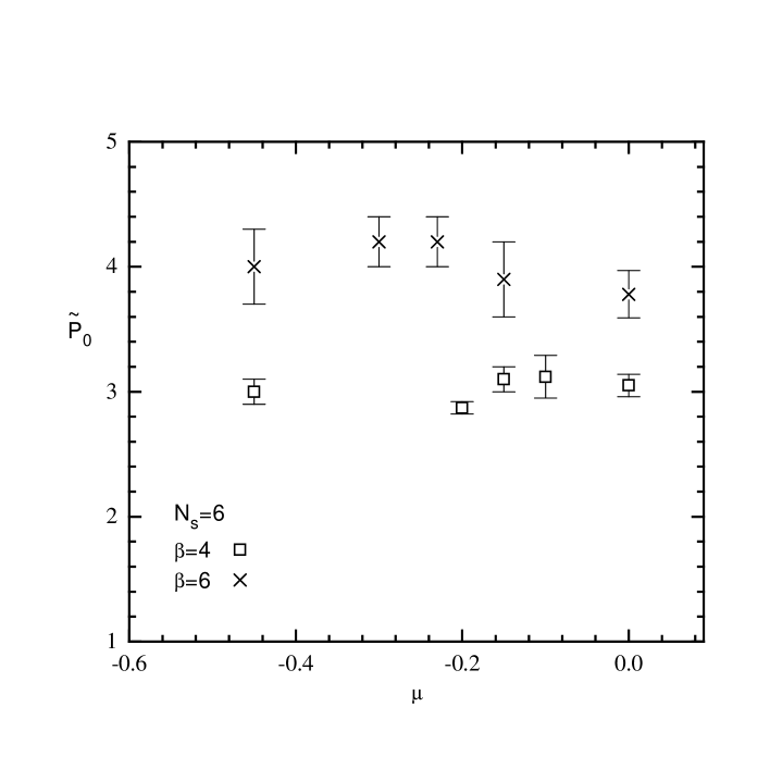
Figure 1: $\widetilde{P}_{0}$ as a function of $\mu$ for $U=4$.

In order to probe such a behavior, we select out from our data of Table (4) the values of $\widetilde{P}_{0,N_{s}}$ obtained at the largest $\beta$ (4 and 6) and $N_{s}=6$ available for a sufficient range of $\mu$ values. The result is shown in Fig. (1). These data are compatible with $\widetilde{P}_{0,N_{s}}$ being constant with respect to $\mu$, and not compatible with a sharp maximum in this $\mu$ range (corresponding to a filling between .65 and 1.0 for both $\beta$ values), as suggested in Ref. [5].

We may still examine the dependence of $\widetilde{P}_{0,N_{s}}$ on $N_{s}$ at fixed $\mu$, to see if these data give evidence for a KT transition at $\mu\neq 0$. We therefore fix $\mu$ at -0.15, a value at which we have data in the range $1\leq\beta\leq 6$ and for various $N_{s}$ values in the 4-8 range.

Let us first assume that at each $\beta$ the largest $N_{s}$ value available is large enough for the system to be close to its thermodynamical limit, an assumption which is verified at $\beta=4$ as seen from our data at $N_{s}=4,6,8$. In Fig. (2) we show $\widetilde{P}_{0,N_{s}}$ as a function of $T$ for $N_{s}=4$ at $\beta\leq 3$ and $N_{s}=8$ for $\beta\geq 4$, together with a fit to Eqs. (54, 55) (continuous line). The fit is remarkably good in the entire temperature range. It favors a KT transition at $T_{\rm KT}=.03(2)$, at about 4 standard deviations away from the value .1 preferred in Ref. [5]. Also shown is a fit to Eqs. (52, 53) (dotted line), which is compatible as well with the data, provided the $T=1$ point is ignored. Imposing $T_{\rm KT}=0.1$ gives poor fits (see Table (6)).

These fits provide us with a guess for the parameterization of the correlation length, up to a normalization factor, which allows us to test scaling behavior given by (57) or (56). With the parameters of lines 1 and 4 of Table (6), we obtain the results shown in Figs. (3) and (4) respectively, together with the asymptotic limits $c(N_{s}/\xi_{\rm KT})^{-1.75}$ and $c^{\prime}(N_{s}/\xi)^{-2}$ expected in the infinite volume limit for the scaling functions $f_{\rm KT}$ and $f$ ($c$ and $c^{\prime}$ are determined by the $\beta=3$, $N_{s}=4$ point). Since both figures may be considered as suggestive of a scaling behavior, the evidence for a Kosterlitz-Thouless transition at $\mu=-0.15$ remains poor.

From this analysis, our conclusion is: If there is a Kosterlitz-Thouless transition for $U=4$, $\mu=-0.15$, it occurs at such a small value of $T$ in units of the hopping parameter $k$ (a few percent) that its effects are hardly distinguishable from those of the $T=0$ singularity expected at $\mu=0$. (Eq. 52).

This conclusion is different from that of [5], and one must try to understand why. At the quantitative level, for $U=4$, the values we find for $\widetilde{P}_{0,N_{s}}$ at $\mu=-0.15$ above $\beta=3$ are smaller than in [5] at $\left<n\right>=0.87$, especially at $\beta=6$. That $\left<n\right>$ depends on $N_{s}$ at fixed $\mu$ as already mentioned (see Table (4)) is insufficient to explain the difference since we do not observe significant $\mu$ dependence in $\widetilde{P}_{0,N_{s}}$.

Of course larger $\widetilde{P}_{0}$ values at a given $\beta$ favor larger $T_{\rm KT}$ when analyzed in terms of the (57) Ansatz, and this may explain the value $T_{\rm KT}\sim.1$ proposed in [5]. However, we would like to point out that the data corresponding to the highest $\beta$ values 8 and 10 of the latter reference were not used in the finite size analysis provided there. A look at these data strongly suggests that including them would have considerably lowered the guessed value of $T_{\rm KT}$.

We did not take enough data at $U=2$ and $U=8$ to allow for an analysis similar to that achieved at $U=4$. A look at Table (5) however confirms that the pair correlation increases with $\beta$ at fixed $[\mu,U]$, while its values at $\mu=0$ and -0.15 are consistent with each other at fixed $[\beta,U]$. Some information comes from comparing $\widetilde{P}_{0}$ at $U=2,4$ and $8$ for $\beta=2$ and $\mu=0.$ fixed. Its values are respectively 1.127(4), 1.63(3) and 2.2(2). It would be incorrect to directly infer from this that also the correlation length increases. In fact, as $U$ increases at fixed temperature, more pairs are formed and this affects the normalization of the correlation function. As a measure of this normalization we take the $x=y$ (zero distance) value of the correlation of Eq. (7),

$$P(0)=\left<a_{x}^{\dagger}b_{x}^{\dagger}b_{x}a_{x}+b_{x}a_{x}a_{x}^{\dagger}b_{x}^{\dagger}\right>\hskip 12.0pt,$$ (58)

which is nothing but the average number densities of doubly occupied and empty sites, related to the single occupation probability $S_{1}$, given in Tables (4,5), by $P(0)=1-S_{1}$. Hence a better representative of the correlation length variations is $\widetilde{P}_{0}/P(0)$, and for this quantity at $\beta=2,\mu=0,U=2,4,$ and 8 respectively we find 1.80(2), 2.18(4) and 2.4(2).

This leaves uncertain the guess that the correlation length is larger at $U=8$ than it is at $U=4$.

The above remark about the normalization of $\widetilde{P}_{0}$, which might be important for a discussion of the $U$ dependence of the KT transition temperature, does not alter our previous analysis at $U=4$ fixed because, as seen from Table (4), $P(0)$ is essentially insensitive to $\beta$, $\mu$ and $N_{s}$ in the explored ranges. This is true even at temperatures as high as 1 at $U=2$ and 4. The largest variation observed for $P(0)$ is found between $T=0.5$ and $T=2$, for $U=8$, where it however does not exceed 10%. So, in the $U$ ( and $\mu$) range considered, the pairs are very robust against temperature rises.

The independence of $S_{1}$ on the filling for fixed $U$ in the region we investigated means that the increase in the filling goes into the formation of pairs. This is, however, also true in the free case in this region. This may be related to the fact that $S_{1}$, as well as $\widetilde{P}_{0}$, is an even function of $\mu$.

6. The susceptibility: Comparison of numerical results with hopping parameter expansion

The free energy of the repulsive Hubbard model has been expanded in powers of the hopping parameter $k$ by various authors [14, 15, 16, 3]. We start from the result of [3], where the expansion is pushed to order 5 in $k^{2}$. Via a particle-hole transformation on one of the two electron operators, the free energy expansion is transformed into that relevant for the Hamiltonian in the attractive case Eq. (1). For arbitrary values of $\beta^{-1}$, $\mu$ and $h$ respectively of the temperature, chemical potential and external magnetic field, we end up with the following truncated expansion ( $F$ is the negative of $\beta$ times the free energy density)

$$F(\beta,U,\mu,h) \equiv \frac{1}{V}\mbox{ln}Z+O(k^{12})$$ (59)

$$= \mbox{log}z+\sum\limits_{\kappa=1}^{5}\sum\limits_{\left\{R\right\}}\frac{v^{2\kappa}}{\left(\beta U\right)^{i}}x^{i_{\mu}}y^{i_{h}}x^{i_{w}}C_{\kappa;\left\{R\right\}}\hskip 12.0pt,$$

where

$$x=e^{\beta\mu},y=e^{\beta h},w=\exp\left[-\frac{\beta U}{2}\right]$$

$$v=\frac{\beta k}{z}$$

$$z=1+xw\left(y+1/y\right)+x^{2}\hskip 12.0pt.$$ (60)

and $\left\{R\right\}$ represents the set of integers $\left\{i,i_{\mu},i_{h},i_{w}\right\}$.

The symbol $C_{\kappa,\left\{R\right\}}$ represents the 3836 non zero coefficients provided in [3], labeled by the order $\kappa$ in $k^{2}$ and the associated set $\left\{R\right\}$. By differentiation with respect to $\mu$ and $h$, one obtains similar series (here taken at zero magnetic field) for the filling density, the static uniform charge density correlation and the static uniform spin susceptibility. We focus on the latter, and study the truncated series

$$\frac{1}{\beta}\widetilde{\chi}(q=0)=\left(y\frac{\mbox{d}}{\mbox{d}y}\right)^{2}F\equiv\sum\limits_{\kappa=0}^{5}A_{\kappa}k^{2\kappa}\hskip 12.0pt.$$ (61)

The coefficients $A_{\kappa}$ follow from the expansion (59) of $F$. Although it is not strictly speaking a high temperature series, but a series in $(\beta k^{2})$ with $\beta$-dependent coefficients, extracting information from such short expansions at low temperature is notoriously difficult.

An idea of the problem at hand is given by the following examples. We take $U=4$, $\mu=0$ and compute the coefficients $A_{\kappa}$ for $\beta=1$ and $2$. Their numerical ratios to $A_{0}$ are shown in Table (7).

One observes a quite discouraging pattern of orders of magnitude and signs (remember we want to evaluate $\widetilde{\chi}$ at $k=1$). We tried to understand what happens by starting from the free case $U=0$, at $\mu=0$. The exact susceptibility is given by (see appendix A)

$$\widetilde{\chi}=\beta\int\limits_{0}^{\pi}\frac{\mbox{d}p_{1}\mbox{d}p_{2}}{\pi^{2}}\frac{1}{1+\mbox{cosh}(2k\beta\delta_{p})}$$ (62)

with

$$\delta_{p}=-(\mbox{cos}p_{1}+\mbox{cos}p_{2})\hskip 12.0pt.$$ (63)

Its expansion in $(\beta k)^{2}$ to $5^{th}$ order is found to be

$$\frac{2\widetilde{\chi}}{\beta}=1-(\beta k)^{2}+\frac{3}{2}(\beta k)^{4}-\frac{85}{36}(\beta k)^{6}+\frac{1085}{288}(\beta k)^{8}-\frac{4837}{800}(\beta k)^{10}$$ (64)

The signs now alternate, but again the size of the coefficients in $k^{2}$ increases fast, the more so the temperature is lowered. Here the origin of this blow up is clear from expression (62). Rewriting it as

$$\frac{\widetilde{\chi}}{\beta}=\int\limits_{0}^{2}\mbox{d}\delta\rho(\delta)\frac{1}{1+\mbox{cosh}\left(2k\beta\delta\right)}$$ (65)

where $\rho(\delta)$ represents the density of states, and recalling that $\rho$ has only a logarithmic (van Hove) singularity at $\delta=0$, all singularities of $\widetilde{\chi}$ in $k$ at finite distance are end point ($\delta=2$) singularities. They are located at $\mbox{cosh}(4k\beta)=-1$, and the closest one, which fixes the radius of convergence, is at $(\beta k)^{2}=-\pi^{2}/16$. Hence the alternate signs in the above series and also the fact that $\pi^{2}/16$ times the ratio $|A_{5}/A_{4}|$ is very close to 1 (namely .990) . Finally, we note from the above integral that the most singular part of $\widetilde{\chi}/\beta$ is proportional to $\mbox{tanh}(2\beta k)/(\beta k)$. This leads us to perform the change of variable $\beta k\to u$ defined by

$$u=\mbox{tanh}\left(2\beta k\right)/(\beta k)-2\hskip 12.0pt,$$ (66)

and to re-expand $\widetilde{\chi}/\beta$ in powers of $u$. We find

$$\frac{2\widetilde{\chi}}{\beta}=1+\frac{3u}{8}-\frac{9u^{2}}{640}+\frac{246u^{3}}{51469}-\frac{4096u^{4}}{2238401}+\frac{30034u^{5}}{40581943}+\cdots$$ (67)

that is

$$\frac{2\widetilde{\chi}}{\beta}\simeq 1.+.375u-1.41\;10^{-2}u^{2}+4.78\;10^{-3}u^{3}-1.83\;10^{-3}u^{4}+7.40\;10^{-4}u^{5}$$ (68)

The interval $\beta k\geq 0$ is mapped onto $-2\leq u\leq 0$, and low temperatures mean $u\sim-2$. Clearly this series in $u$ looks much more tractable than the original one. Indeed, actual comparison of Padé approximants of (68) with the exact result (62) shows that, up to $\beta\sim 10$, the latter can be approached with an accuracy better than 5%, an achievement not expected from the series (64)!

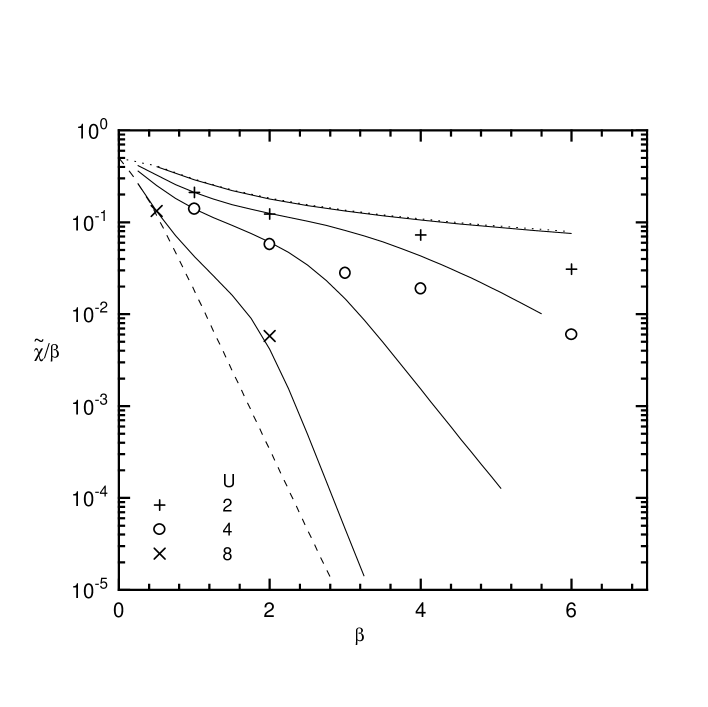
Figure 5: $\widetilde{\chi}/\beta$ as a function of $\beta$ for different values of the coupling $U$ at $\mu=0$. See description in the text.

In the absence of any information on the analytic structure of $\widetilde{\chi}$ in $k$ as the interaction is turned on, we decided to perform the same change of variable (66) in all cases and constructed the Padé approximants to the series in $u$. We observe that the [2,3] and [3,2] approximants systematically lead to very similar results. Our results for $\mu=0$ are collected in Fig. (5), and compared with those of the numerical simulation, as obtained with the largest lattices which were simulated for each set of $\beta,U$ values. We now describe and comment this figure.

The upper (dotted) curve is the exact result in the free case $U=0$. The four continuous lines are the [2,3] Padé results for respectively $U=0.1,2,4,8$, from top to bottom . The lower (dashed) line is the “atomic” limit $(k=0)$ drawn for $U=8$. The statistical errors are smaller than the size of the symbols representing our numerical results for the largest available values of $N_{s}$, $N_{t}$. Tables (4,5, 8) show that sizable finite size effects are present. In particular, unlike $\widetilde{P}_{0}$, the susceptibility appears to be rather sensitive to the number $N_{t}$ of time slices. When comparisons can be made, our results are in general agreement with published data [17, 5, 18].

The $U=0.1$ curve is used as an overall check that the whole series constructed from [16] is correctly implemented and that the change of variable and Padé reconstruction work close to the free case. For $U=2$, excellent agreement between series and data is obtained at $\beta=1$ and $2$. The figure suggests that at $\beta=3$, the series still gives a reasonable answer, although lower than the true one by probably 10 to 15 %. A similar departure shows up above $\beta=2$ at $U=4$, and, say, $\beta=1.5$ at $U=8$. Hence the overall pattern is that our treatment of the series gives good results at $\beta$ values below a maximum which decreases as $U$ increases. Above this maximum, the Padé approximant drops down rapidly the more so when $U$ is large. It is interesting to discuss this latter feature. Consider again the case $U=8$. The dashed line $(k=0)$ is the curve (see appendix A)

$$\frac{\widetilde{\chi}}{\beta}=\frac{w}{1+w}\mbox{ , }w=\exp\left[-\beta U/2\right]\hskip 12.0pt,$$ (69)

drawn for $U=8$, thus falling down like $\exp\left[-4\beta\right]$. One observes that the Padé result at $U=8$ drops down roughly parallel to it above $\beta=2$.

Inspection of the series for $\widetilde{\chi}$ reveals that all (known) terms of its expansion in $k^{2}$ contain at least one power of $w$ as a factor. So any truncation unavoidably leads to an exponential fall off in $\beta$ at fixed $U$, the more so when $U$ is large. This is what we observe with the series at hand, while the numerical simulation indicates that, although $\widetilde{\chi}$ actually decreases as $\beta$ increases, it does so at a much slower rate than naively expected. In other words, there are collective effects which rather tend to maintain a sizable susceptibility, even though low temperature or/and large $U$ favor the formation of local pairs, which contribute zero to the total spin. We note that, as already mentioned in the previous section, the probability for single occupation, $S_{1}$ (as given in Tables (4,5)) and thus the average local pair number $\left<n/2\right>-S_{1}/2$, depends weakly upon temperature. Hence the decrease of $\widetilde{\chi}$ with $T$ is not a consequence (only) of pair formation at fixed $U$ and $\left<n\right>$. Its sensitivity to $U$ also is strong compared to that of $S_{1}$. As recently discussed in [18], these questions are of interest in connection with the kind of regime (BCS-like or pair condensation) eventually leading to a superconducting transition. See also [5, 17].

Our results show that, unlike popular approximations such as RPA or T–matrix treatment, the series expansion in $k^{2}$ can be continued successfully down to fairly small $T$ values even at large coupling. In order to further illustrate this point, we present our predictions for $\widetilde{\chi}$ as a function of $T$ for $U$ = 4, 6, 8 and 12, at half filling ($\left<n\right>=1$), in Fig. (6). These predictions appear as solid lines when our calculation is accurate (the minimum $T$’s of the solid lines are conservative guesses). We point out that by themselves these results clearly expose the main features of physical interest, namely the existence of a crossover from a smooth regime at high $T$ to a rapid fall off below a $U$ dependent $T$ value. Furthermore, we observe that these $\widetilde{\chi}$ values are quantitatively very close to that of [18] obtained numerically at the same $U$ values, but for $\left<n\right>=0.8$. This enforces our general statement that there is no evidence for any substantial dependence on filling.

7. Summary and conclusion

Motivated by the interest for strongly interacting systems of electrons in the context of high $T_{c}$ materials, we have performed an investigation of the attractive Hubbard model.

Based on the hybrid Monte-Carlo method to simulate the path integral representation of the partition function, a numerical study provided us with estimates of the static zero-momentum pair correlation $\widetilde{P}_{0}$ and spin susceptibility $\widetilde{\chi}$. The exploration covered the ranges [0.5, 6.0] for the inverse temperature $\beta$ and [2.0, 8.0] for the interaction strength $U$ in units of the hopping parameter $k$. At $U$=4 we investigate in detail the dependence on the chemical potential in order to study the sensitivity of these physical quantities to band filling, at and away from half filling. We also performed an analytical investigation of the susceptibility, based on its expansion in $k^{2}$ to order 5 derived from the results of [3] and on a specific Padé resummation technique inspired by the free case. We show that this method yields very good results for $\beta\mathchar 13358\relax 1$ at any $U$, and $\beta\mathchar 13358\relax 2$ for $U\mathchar 13358\relax 4$.

In the numerical approach, the cost in computer time leads to the consideration of rather small lattices only, and also limits the number of time slices involved. The limitation of the analytical approach is obviously due the truncation of the $k^{2}$ expansion, which furthermore is not available for the pair correlation. But it yields estimates of $\widetilde{\chi}$ directly in the thermodynamical limit, so that the two approaches are complementary and their comparison brings valuable information. Whenever it was possible, we also compared our numerical data with those of previous investigations [5, 4, 18] performed using Quantum Monte-Carlo. The overall agreement is good, although we found significant discrepancies for $\widetilde{P}_{0}$ at our lowest T values.

Using pair correlations, the main question addressed was that of the existence and location $T_{\rm KT}$ of a Kosterlitz-Thouless superconducting transition, the only possible transition at finite temperature away from half filling. Our results show very weak dependence on $\mu$, hardly distinguishing half filling from other values of band filling in the range between $.4$ and $.5$. Fits or finite size analysis relevant to a KT transition are consistent with a transition at $T_{\rm KT}/k$ of the order of a few percent, with a weak dependence on $\mu$, if any. This conclusion is at variance with that drawn in [5], but we point out that it is perhaps consistent with what might follow from taking into account the lowest temperature data points of this latter reference. In any case, from our analysis we conclude that it is always necessary to compare quantitatively the behavior at $\mu=0$, where there should not be a transition at finite T to $\mu\neq 0$, before one can ascertain the existence of a KT transition at finite T, and estimate its critical temperature.

Our study of the magnetic susceptibility shows that it depends very weakly on the band filling, but decreases rapidly with increasing $U$ and/or decreasing temperature, in agreement with previous investigations [17, 5, 18]. Increasing $U$ favors S-wave pair formation, reducing the probability $S_{1}$ of sites occupied by a single electron responding to a magnetic field. This explains the simultaneous decrease of $\widetilde{\chi}$ and $S_{1}$ at fixed temperature. But at fixed $U$, we observe that $S_{1}$ stays approximately constant in the low temperature range whereas $\widetilde{\chi}$ falls steeply. This casts some doubt on the existence of a tight connection between susceptibility and pair formation as the expected transition is approached as claimed in [18].

In this work, we restricted our data analysis to static, zero momentum correlations. However, we have stored all the information required to also analyze spatial correlations and investigate dynamical properties of the model.

Appendix A

We first discuss the atomic case $k=0$, at $h=0$

$$H=-U\left(a^{\dagger}a-\frac{1}{2}\right)\left(b^{\dagger}b-\frac{1}{2}\right)-\mu\left(a^{\dagger}a+b^{\dagger}b\right)\hskip 12.0pt.$$ (70)

There are only 4 states. It is convenient to introduce the variables

$$x=e^{\beta\mu}\hskip 12.0pt,$$ (71)

$$w=e^{-\frac{\beta U}{2}}\hskip 12.0pt.$$ (72)

One easily finds

$$Z=1+2wx+x^{2}\hskip 12.0pt,$$ (73)

$$\left<n\right>=\frac{2x\left(w+x\right)}{1+2wx+x^{2}}\hskip 12.0pt,$$ (74)

$$\widetilde{P}_{0}=\frac{1+x^{2}}{1+2wx+x^{2}}\hskip 12.0pt,$$ (75)

$$\widetilde{\chi}=\beta\frac{2wx}{1+2wx+x^{2}}\hskip 12.0pt,$$ (76)

$$\widetilde{C}(0,0)=\frac{2x\left(w+2x\right)}{1+2wx+x^{2}}\hskip 12.0pt.$$ (77)

The single occupation probability is

$$S_{1}=\frac{2xw}{1+2wx+x^{2}}=\frac{\widetilde{\chi}}{\beta}\hskip 12.0pt.$$ (78)

One remarks that $\widetilde{P}_{0}$ is always smaller than 1. The path integral expression of $Z$ factorises into one path integral for every site. It can be analytically calculated, and with the form of the action which we use, the result is exact independent of the value of $N_{t}$, i.e. there are no finite $N_{t}$ corrections.

In the free case $U=0$, the Hamiltonian, diagonalized in momentum space, is

$$H_{U=0}=\sum_{p}(\epsilon_{p}-\mu)(\tilde{a}_{p}^{\dagger}\tilde{a}_{p}+\tilde{b}_{p}^{\dagger}\tilde{b}_{p})-h(\tilde{a}_{p}^{\dagger}\tilde{a}_{p}-\tilde{b}_{p}^{\dagger}\tilde{b}_{p})\hskip 12.0pt,$$ (79)

where $\epsilon_{p}=-2k(\cos p_{1}+\cos p_{2})$ for momenta $p=(p_{1},p_{2})$ and $h$ is the magnetic field introduced for completeness.

On a finite lattice $p_{i}=\frac{2\pi}{N_{s}}n_{i}$, $n_{i}=1,2,\cdots,N_{s}$. The correspondence with the thermodynamical limit $N_{s}\longrightarrow\infty$ is given by

$$\frac{1}{N_{s}^{2}}\sum_{p}\longleftrightarrow\int_{0}^{2\pi}\frac{dp_{1}dp_{2}}{4\pi^{2}}\hskip 12.0pt.$$ (80)

Setting

$$s_{p}=\exp[-\beta(\epsilon_{p}-\mu)]\hskip 12.0pt,$$ (81)

one derives the partition function

$$Z=\prod_{p}(1+s_{p}{\rm e}^{\beta h})(1+s_{p}{\rm e}^{-\beta h})\hskip 12.0pt,$$ (82)

and the zero field quantities of interest :

$$\left<n\right>=\frac{2}{N_{s}^{2}}\sum_{p}\frac{s_{p}}{1+s_{p}}\hskip 12.0pt,$$ (83)

$$\widetilde{P}_{0}=\frac{1}{N_{s}^{2}}\sum_{p}\frac{1+s_{p}^{2}}{(1+s_{p})^{2}}\hskip 12.0pt,$$ (84)

$$\widetilde{\chi}=\beta\frac{2}{N_{s}^{2}}\sum_{p}\frac{s_{p}}{(1+s_{p})^{2}}\hskip 12.0pt,$$ (85)

$$\widetilde{C}(0,0)=\frac{2}{N_{s}^{2}}\sum_{p}\frac{s_{p}(1+2s_{p})}{(1+s_{p})^{2}}\hskip 12.0pt.$$ (86)

The single occupation probability $S_{1}=\left<n\right>-\left<n\right>^{2}/2$ is independent of temperature at fixed filling. It varies from 0 at zero filling to 1/2 at half filling.

Using $s_{p}=1/s_{p-(\pi,\pi)}$ at $\mu=0$, the susceptibility at half-filling becomes

$$\left.\frac{\widetilde{\chi}}{\beta}\right|_{\mu=0}=\frac{1}{N_{s}^{2}}\sum_{p}\frac{1}{1+\cosh(\beta\epsilon_{p})}\hskip 12.0pt.$$ (87)

Appendix B

In order to include terms of order $1/N_{t}^{2}$ within the action, we apply a Trotter-splitting in the following way:

$$e^{-\frac{\beta}{N_{t}}\left(H_{K}+H_{V}\right)}=e^{-\frac{\beta}{2N_{t}}H_{K}}e^{-\frac{\beta}{N_{t}}H_{V}}e^{-\frac{\beta}{2N_{t}}H_{K}}+O\left(\frac{1}{N_{t}^{3}}\right)\hskip 12.0pt,$$ (88)

where

$$H_{K}=-k\sum_{\left<x,y\right>}\left(a^{\dagger}_{x}a_{y}+a^{\dagger}_{y}a_{x}+b^{\dagger}_{x}b_{y}+b^{\dagger}_{y}b_{x}\right)\hskip 6.0pt,$$ (89)

and

$$H_{V}=-U\sum_{x}\left(a^{\dagger}_{x}a_{x}-\frac{1}{2}\right)\left(b^{\dagger}_{x}b_{x}-\frac{1}{2}\right)-\mu\sum_{x}\left(a^{\dagger}_{x}a_{x}+b^{\dagger}_{x}b_{x}\right)\hskip 6.0pt.$$ (90)

We then, as before, introduce an auxiliary scalar field. Then we expand the three exponentials in (88), collect terms including order $1/N_{t}^{2}$ and write the summands of operators in normal order. In the resulting expression we can substitute the operators by Grassmann variables. The procedure described gives rise to additional terms in the action. The spatial elements of the matrix in Eq. (26) now read

$$M_{x,t;y,t} = \frac{k\beta}{2N_{t}}\sum\limits_{\hat{\nu}=\hat{1}}^{\hat{2}}\left(\delta_{y,x+\hat{\nu}}+\delta_{y,x-\hat{\nu}}\right)\times$$

$$\times \left\{\exp\left[\sqrt{\frac{U\beta}{N_{t}}}\sigma_{x,t}-(U-\mu)\frac{\beta}{N_{t}}\right]+\exp\left[\sqrt{\frac{U\beta}{N_{t}}}\sigma_{y,t}-(U-\mu)\frac{\beta}{N_{t}}\right]\right\}$$ (91)

$$+ \delta_{x,y}\left\{\exp\left[\sqrt{\frac{U\beta}{N_{t}}}\sigma_{x,t}-(U-\mu)\frac{\beta}{N_{t}}\right]-1\right\}$$

$$+ \frac{k^{2}\beta^{2}}{2N_{t}^{2}}\sum\limits_{\hat{\nu},\hat{\nu}^{\prime}=\hat{1}}^{\hat{2}}\left\{\delta_{y,x+\hat{\nu}+\hat{\nu}^{\prime}}+\delta_{y,x-\hat{\nu}-\hat{\nu}^{\prime}}+2\delta_{y,x+\hat{\nu}-\hat{\nu}^{\prime}}\right\}\hskip 12.0pt.$$

Lattice	$U$	$\beta$	$-\mu$	$\tau$	$n_{\rm MD}$	Traj.	$\xi_{\sigma^{\prime}}$	Acc.
$4^{2}\times 16$	4	1	.15	1.6	16	19270	37	.99
$4^{2}\times 8$	4	1	.15	1.6	16	20000	23	.99
$6^{2}\times 8$	4	1	.15	1.6	16	20000	21	.98
$4^{2}\times 16$	4	1	.0	1.6	16	19160	38	.99
$4^{2}\times 8$	4	1	.0	1.6	16	20000	23	.99
$6^{2}\times 16$	4	1	.0	1.6	16	20000	36	.98
$6^{2}\times 8$	4	1	.0	1.6	16	20000	22	.98
$4^{2}\times 16$	4	2	.15	1.6	32	12500	33	.98
$4^{2}\times 16$	4	2	.0	1.6	32	12500	33	.98
$4^{2}\times 24$	4	3	.15	1.6	48	12250	81	.95
$4^{2}\times 24$	4	3	.0	1.6	48	12500	54	.95
$4^{2}\times 32$	4	4	.6	0.8	64	22500	91	.99
$4^{2}\times 32$	4	4	.45	0.8	64	22210	191	.99
$6^{2}\times 32$	4	4	.45	1.6	64	20970	43	.85
$6^{2}\times 32$	4	4	.2	1.6	64	43340	158	.83
$4^{2}\times 32$	4	4	.15	0.8	64	19800	290	.98
$6^{2}\times 32$	4	4	.15	1.6	64	20220	67	.82
$8^{2}\times 32$	4	4	.15	1.6	64	18490	126	.71
$6^{2}\times 32$	4	4	.1	1.6	64	20530	50	.82
$4^{2}\times 32$	4	4	.0	0.8	64	19960	228	.98
$4^{2}\times 64$	4	4	.0	1.6	64	20000	121	.94
$6^{2}\times 32$	4	4	.0	1.6	64	20270	82	.84
$4^{2}\times 64$	4	6	.45	1.2	96	10000	127	.98
$6^{2}\times 64$	4	6	.45	1.2	96	9200	109	.88
$4^{2}\times 64$	4	6	.3	1.2	96	12500	292	.96
$6^{2}\times 64$	4	6	.3	1.2	96	12500	146	.87
$6^{2}\times 64$	4	6	.23	1.2	96	12500	170	.85
$4^{2}\times 64$	4	6	.15	1.2	96	19300	335	.96
$6^{2}\times 64$	4	6	.15	1.2	96	12500	565	.85
$8^{2}\times 64$	4	6	.15	1.2	96	8200	250	.64
$4^{2}\times 64$	4	6	.08	1.2	96	20000	743	.96
$4^{2}\times 64$	4	6	.0	1.2	96	12500	185	.97
$6^{2}\times 64$	4	6	.0	1.2	96	10000	179	.85

Table 1: Parameters of the simulations performed at $U=4$. Also given are the number of trajectories generated, the $\sigma^{\prime}$ field autocorrelation time $\xi_{\sigma^{\prime}}$ and the acceptance.

Lattice	$U$	$\beta$	$-\mu$	$\tau$	$n_{\rm MD}$	Traj.	$\xi_{\sigma^{\prime}}$	Acc.
$4^{2}\times 8$	2	1	.0	1.6	8	20000	13	.98
$4^{2}\times 16$	2	2	.0	1.6	16	9230	15	.98
$6^{2}\times 32$	2	4	.15	1.6	32	16140	18	.96
$6^{2}\times 16$	2	4	.15	1.6	32	47000	13	.90
$6^{2}\times 32$	2	4	.0	1.6	32	47180	20	.96
$6^{2}\times 16$	2	4	.0	1.6	32	38000	13	.90
$6^{2}\times 24$	2	6	.3	1.6	48	17780	13	.84
$6^{2}\times 24$	2	6	.15	1.6	48	16810	28	.79
$6^{2}\times 24$	2	6	.0	1.6	48	23420	24	.77
$6^{2}\times 32$	8	0.5	.15	1.6	16	20700	240	.99
$6^{2}\times 32$	8	0.5	.0	1.6	16	20500	162	.99
$6^{2}\times 32$	8	2.0	.15	1.6	64	12612	1237	.95
$6^{2}\times 32$	8	2.0	.0	1.6	64	18855	782	.94

Table 2: Parameters of the simulations performed at $U=$ 2 and 8. Also given are the number of trajectories generated, the $\sigma^{\prime}$ field autocorrelation time $\xi_{\sigma^{\prime}}$ and the acceptance.

Lattice	$U$	$\beta$	$\mu$	order	$\left<\sigma^{\prime}\right>$	$\left<n\right>/2$	$\ \ \widetilde{P}_{0}$	$\widetilde{\chi}\times 10$
$4^{2}\times 16$	4	1	0.	1	1.76(1)	0.468(2)	1.060(2)	1.406(3)
$4^{2}\times 48$	4	1	0.	1	1.94(2)	0.492(4)	1.060(3)	1.398(3)
$4^{2}\times 8$	4	1	0.	2	2.05(2)	0.501(4)	1.071(4)	1.301(8)
$4^{2}\times 16$	4	1	0.	2	1.96(3)	0.490(5)	1.062(5)	1.390(9)
$4^{2}\times 32$	4	4	0.	1	1.34(2)	0.401(3)	2.20(3)	0.81(1)
$4^{2}\times 64$	4	4	0.	1	1.66(3)	0.451(6)	2.27(6)	0.79(2)
$4^{2}\times 32$	4	4	0.	2	2.11(4)	0.514(4)	2.37(9)	0.51(2)
$4^{2}\times 64$	4	4	0.	2	1.98(3)	0.495(5)	2.55(9)	0.71(2)

Table 3: Comparison of data taken with the fermionic matrix to order 1 and 2 in 1/$N_{t}$. See Eqs. (26) and (Appendix B) respectively.

Lattice	$U$	$\beta$	$-\mu$	$\left<\sigma^{\prime}\right>$	$\left<n\right>/2$	$\ \ \widetilde{P}_{0}$	$\widetilde{\chi}\times 10$	$S_{1}$
$4^{2}\times 8$	4	1	.15	1.90(2)	.463(4)	1.072(4)	1.289(8)	.250(2)
$4^{2}\times 8$	4	1	.0	2.05(2)	.501(4)	1.071(4)	1.301(8)	.252(2)
$6^{2}\times 8$	4	1	.15	1.91(1)	.463(2)	1.079(7)	1.300(8)	.253(1)
$6^{2}\times 8$	4	1	.0	2.03(2)	.496(3)	1.075(6)	1.313(8)	.255(1)
$4^{2}\times 16$	4	2	.15	1.81(3)	.440(5)	1.64(2)	1.16(2)	.240(2)
$4^{2}\times 16$	4	2	.0	2.02(3)	.494(4)	1.63(3)	1.18(2)	.244(2)
$4^{2}\times 24$	4	3	.15	1.81(3)	.435(3)	2.18(5)	0.85(3)	.234(2)
$4^{2}\times 24$	4	3	.0	2.10(3)	.509(6)	2.23(5)	0.87(2)	.242(2)
$4^{2}\times 32$	4	4	.6	1.31(2)	.309(1)	2.47(7)	0.45(2)	.226(4)
$4^{2}\times 32$	4	4	.45	1.40(3)	.335(2)	2.6(1)	0.46(2)	.234(1)
$4^{2}\times 32$	4	4	.15	1.87(6)	.45(1)	2.40(6)	0.55(2)	.234(4)
$4^{2}\times 32$	4	4	.0	2.11(4)	.514(4)	2.37(9)	0.51(2)	.230(4)
$6^{2}\times 32$	4	4	.45	1.38(1)	.329(1)	3.0(1)	0.72(1)	.226(1)
$6^{2}\times 32$	4	4	.2	1.74(2)	.422(2)	2.87(5)	0.697(9)	.234(1)
$6^{2}\times 32$	4	4	.15	1.83(2)	.443(2)	3.1(1)	0.68(1)	.232(2)
$6^{2}\times 32$	4	4	.1	1.92(1)	.468(2)	3.1(2)	0.71(1)	.234(1)
$6^{2}\times 32$	4	4	.0	2.06(2)	.501(3)	3.05(9)	0.75(1)	.239(1)
$8^{2}\times 32$	4	4	.15	1.86(2)	.449(2)	2.85(8)	0.72(1)
$4^{2}\times 64$	4	6	.45	1.31(3)	.321(2)	2.38(8)	0.14(2)	.246(6)
$4^{2}\times 64$	4	6	.3	1.41(4)	.344(2)	2.9(1)	0.22(2)	.242(6)
$4^{2}\times 64$	4	6	.15	1.61(4)	.396(3)	3.3(2)	0.23(2)	.234(4)
$4^{2}\times 64$	4	6	.08	1.86(6)	.460(7)	2.58(9)	0.18(1)	.222(4)
$4^{2}\times 64$	4	6	.0	2.03(4)	.503(7)	2.57(9)	0.17(2)	.236(6)
$6^{2}\times 64$	4	6	.45	1.32(2)	.322(2)	4.0(3)	0.38(3)	.224(6)
$6^{2}\times 64$	4	6	.3	1.46(2)	.359(1)	4.2(2)	0.37(4)	.240(4)
$6^{2}\times 64$	4	6	.23	1.62(2)	.396(1)	4.2(2)	0.42(2)	.244(4)
$6^{2}\times 64$	4	6	.15	1.83(5)	.452(2)	3.9(3)	0.31(2)	.238(4)
$6^{2}\times 64$	4	6	.0	2.01(2)	.493(2)	3.8(2)	0.36(3)	.236(4)
$8^{2}\times 64$	4	6	.15	1.75(3)	.429(1)	4.9(4)	0.49(3)	.242(2)

Table 4: Data obtained on various lattices at $U=4$ : $\left<\sigma^{\prime}\right>$, filling of the band $\left<n\right>/2$, pairing correlation $\widetilde{P}_{0}$, spin susceptibility $\widetilde{\chi}$ and single occupation probability $S_{1}$ for different values of the inverse temperature and of the chemical potential.

Lattice	$U$	$\beta$	$-\mu$	$\left<\sigma^{\prime}\right>$	$\left<n\right>/2$	$\ \ \widetilde{P}_{0}$	$\widetilde{\chi}\times 10$	$S_{1}$
$4^{2}\times 8$	2	1	.0	1.45(1)	.502(2)	0.886(1)	2.114(4)	.3738(8)
$4^{2}\times 16$	2	2	.0	1.42(2)	.497(3)	1.127(4)	2.46(1)	.373(1)
$6^{2}\times 32$	2	4	.15	1.268(7)	.438(1)	1.46(1)	2.55(1)	.3732(8)
$6^{2}\times 32$	2	4	.0	1.453(4)	.504(1)	1.445(7)	2.727(9)	.3746(4)
$6^{2}\times 24$	2	6	.3	1.153(4)	.3747(8)	1.99(2)	1.30(2)	.3446(6)
$6^{2}\times 24$	2	6	.15	1.340(8)	.440(2)	2.20(6)	1.69(2)	.3444(8)
$6^{2}\times 24$	2	6	.0	1.605(6)	.531(2)	2.10(3)	1.86(2)	.346(1)
$6^{2}\times 32$	8	.5	.15	2.69(7)	.475(8)	0.948(3)	0.667(5)	.174(2)
$6^{2}\times 32$	8	.5	.0	2.88(6)	.509(8)	0.955(4)	0.661(5)	.173(2)
$6^{2}\times 32$	8	2.	.15	2.3(2)	.41(3)	1.9(1)	0.104(5)	.079(2)
$6^{2}\times 32$	8	2.	.0	2.7(1)	.47(2)	2.2(2)	0.116(5)	.085(2)

Table 5: Data obtained on various lattices at $U=$ 2 and 8. As in Table (4).

fitting function	$b$	$a$	$T_{\rm KT}$	$N_{pts}$	$\chi^{2}/d.o.f.$
$b\exp\left[a/\sqrt{T-T_{\rm KT}}\right]$	0.42(2)	0.92(6)	0.03(2)	5	1.58
	0.46(9)	0.9(2)	0.04(3)	4	2.96
$b\exp\left[a/T\right]$	0.768(8)	0.350(7)		5	10.55
	0.90(3)	0.30(1)		4	1.73
$b\exp\left[a/\sqrt{T-0.1}\right]$	0.545(9)	0.66(1)	0.1	5	16.98
	0.68(3)	0.55(2)	0.1	4	6.02

Table 6: Fits of $\widetilde{P}_{0}$ as a function of $T$ for $U=4$ and $\mu=-0.15$. The point $T=1$ is ignored in every second line. In the last two lines, $T_{\rm KT}$=0.1 [5] is imposed.

$\kappa$	0	1	2	3	4	5
$\beta=1$	1.	.580	-.725	.372	.156	-.497
$\beta=2$	1.	5.65	2.91	-17.6	-.404	62.5

Table 7: The ratios $A_{\kappa}/A_{0}$ of the expansion of $\widetilde{\chi}$ in powers of $k^{2}$ for $U=4$, $\mu=0$, $\beta=1$ and 2.

Lattice	$U$	$\beta$	$-\mu$	$\left<\sigma^{\prime}\right>$	$\left<n\right>/2$	$\ \ \widetilde{P}_{0}$	$\widetilde{\chi}\times 10$	$S_{1}$
$6^{2}\times 32$	2	4	.15	1.268(7)	.438(1)	1.46(1)	2.55(1)	.3732(8)
$6^{2}\times 16$	2	4	.15	1.377(4)	.4514(8)	1.67(1)	2.114(9)	.3510(6)
$6^{2}\times 32$	2	4	.0	1.453(4)	.504(1)	1.445(7)	2.727(9)	.3746(4)
$6^{2}\times 16$	2	4	.0	1.583(4)	.523(1)	1.65(1)	2.212(9)	.3532(6)
$4^{2}\times 16$	4	1	.15	1.81(3)	.453(5)	1.062(5)	1.379(9)	.264(2)
$4^{2}\times 8$	4	1	.15	1.90(2)	.463(4)	1.072(4)	1.289(8)	.250(2)
$4^{2}\times 16$	4	1	.0	1.96(3)	.490(5)	1.062(5)	1.390(9)	.266(2)
$4^{2}\times 8$	4	1	.0	2.05(2)	.501(4)	1.071(4)	1.301(8)	.252(2)
$6^{2}\times 16$	4	1	.0	2.02(2)	.501(3)	1.072(7)	1.382(8)	.267(1)
$6^{2}\times 8$	4	1	.0	2.03(2)	.496(3)	1.075(6)	1.313(8)	.255(1)
$4^{2}\times 32$	4	4	.0	2.11(4)	.514(4)	2.37(9)	0.51(2)	.230(4)
$4^{2}\times 64$	4	4	.0	1.98(3)	.495(5)	2.55(9)	0.71(2)	.244(2)

Table 8: Comparison of data taken at different $N_{t}$ values.

Figure 2: $\widetilde{P}_{0}$ as a function of the temperature for $U=4$ and $\mu=-0.15$. The solid curve is the fit to $\widetilde{P}_{0}=b\exp\left[a/(T-T_{\rm KT})^{1/2}\right]$, the dashed curve is the fit to $\widetilde{P}_{0}=b\exp\left[a/T\right]$. The parameters are given in line 1 and 4 of Table 6.

Figure 3: Scaling of $\widetilde{P}_{0}$ (Eq. (57) ).

Figure 4: Scaling of $\widetilde{P}_{0}$ (Eq. (56) ).

Figure 6: $\widetilde{\chi}$ as a function of $T$ for different values of the coupling $U$ at $\mu=0$. From top to bottom $U=4,6,8$ and $12$. See description in the text.

References

- [1] J.Hubbard, Proc. R.Soc.London A 276 283 (1963); A 281 401 (1964).
- [2] J.M. Kosterlitz and D.J. Thouless, J. Phys. C 6 1181 (1973).
- [3] J. Oitmaa and J.A. Henderson, Aust. J. Phys. 46, 613 (1993).
- [4] R.T. Scalettar, E.Y. Loh, J.E. Gubernatis, A.Moreo, S.R. White, D.J. Scalapino, R.L. Sugar and E. Dagotto, Phys. Rev. Letters 62 1407 (1989).
- [5] A. Moreo and D.J. Scalapino, Phys. Rev. Lett. 66, 946 (1991); A. Moreo, D.J. Scalapino and S.R. White, Phys. Rev. B 45, 7544 (1992).
- [6] C.N. Yang and S.C. Zhang, Modern Physics Letters B4 759 (1990); S.C. Zhang, Phys. Rev. Letters 65 120 (1990).
- [7] M. Creutz, Phys.Rev D 38, 1228 (1988).
- [8] R.Gupta, G.W. Kilcup and S.R. Sharpe, Phys. Rev D 38, 1278 (1988).
- [9] S.Gupta, A. Irbäck, F.Karsch and B.Petersson, Phys. Lett. B 242, 437 (1990).
- [10] P.B. Mackenzie, Phys. Lett. B 226, 369 (1989).
- [11] D. Weingarten, Nucl. Phys. B (Proc.Suppl.) 9, 447 (1989).
- [12] G.H. Golub and C.F. van Loan, Matrix Computations, (Johns Hopkins University Press, Baltimore Maryland, 1983).
- [13] S.R. White, D.J. Scalapino, R.L. Sugar, E.Y. Loh, J.E. Gubernatis, R.T. Scalettar, Phys. Rev. B 40 506 (1989).
- [14] K.K. Pan and Y.L. Wang, Phys.Rev. B 43, 3706 (1991); J. Appl. Phys. 69, 4656 (1991), references to earlier work therein.
- [15] D.F.B. ten Hopf and J.M.S. van Leeuwen, Phys.Rev. B 46, 6313 (1992).
- [16] J.A. Henderson, J. Oitmaa and M.C.B. Ashley, Phys.Rev B 46, 6328 (1992).
- [17] M. Randeria, N. Trivedi, A.Moreo and R.T. Scalettar, Phys. Rev. Letters, 69 2001 (1992).
- [18] J.M. Singer, M.H. Pedersen, T. Schneider, H. Beck and H.G. Matuttis, Phys. Rev. B 54 1286 (1996).