Charge-Relaxation and Dwell Time in the Fluctuating Admittance of a Chaotic Cavity

Abstract

We consider the admittance of a chaotic quantum dot, capacitively coupled to a gate and connected to two electron reservoirs by multichannel ballistic point contacts. For a dot in the regime of weak-localization and universal conductance fluctuations, we calculate the average and variance of the admittance using random-matrix theory. We find that the admittance is governed by two time-scales: the classical admittance depends on the $RC$-time $\tau$ of the quantum dot, but the relevant time scale for the weak-localization correction and the admittance fluctuations is the dwell time. An extension of the circular ensemble is used for a statistical description of the energy dependence of the scattering matrix.

A quantum dot is a small conducting island, formed with the help of gates, with a ballistic and chaotic classical dynamics, and coupled to electron reservoirs by ballistic point contacts. The search for signatures of phase-coherent transport through chaotic quantum dots focused on the d.c. conductance [1, 2, 3, 4]. However, the a.c. response is also of interest [3, 5, 6], since it probes the charge distribution and its dynamics. While the d.c. conductance is entirely determined by the scattering properties of the quantum dot, a.c. transport requires that nearby conductors (gates) are taken into account as well [7, 8, 9]: charges may temporarily pile up in the quantum dot, thus interacting with the gates through long-range Coulomb forces.

Except for highly transmissive samples [9], the low-frequency dynamics of a mesoscopic conductor is governed by a charge-relaxation mode or an RC-relaxation time $\tau$. However, as soon as weak localization [10] and universal conductance fluctuations [11] play a role, this is no longer a complete picture. In this work, we demonstrate that the weak localization effects and the a.c. conductance (admittance) fluctuations are primarily governed by a second time-scale, a dwell time $\tau_{d}$, characteristic of the non-interacting system. The large disparity of these two time-scales ($\tau_{d}\gg\tau$ for a macroscopic quantum dot) dramatically affects the admittance and provides a signature that should be readily observed.

In a recent paper, Gopar, Mello, and one of the authors studied the capacitance fluctuations of a chaotic quantum dot, coupled to the outside world through one point contact with a single conducting channel only [5]. For the low-frequency fluctuations, weak localization effects are absent and the double-time scale behavior discussed here does not occur. In this letter, we calculate the average and variance of the admittance for the case of a two-probe quantum dot with multichannel point contacts. Multichannel contacts are necessary to be in the regime of weak localization and universal conductance fluctuations. Moreover, the presence of two point contacts instead of one turns out to be essential for the existence of quantum interference effects to leading order in the frequency $\omega$.

The system under consideration is depicted in Fig. 1a. Two electron reservoirs at voltages $U_{1}(\omega)$ and $U_{2}(\omega)$ are coupled to the quantum dot by two point contacts with $N_{1},N_{2}\gg 1$ modes, through which currents $I_{1}(\omega)$ and $I_{2}(\omega)$ are passed. The dot is coupled capacitively to a gate, connected to a reservoir at voltage $U_{3}(\omega)$, from which a current $I_{3}(\omega)$ flows. A geometrical capacitance $C$ accounts for the capacitive coupling with the gate [5, 7]. We assume that the gate is macroscopic, i.e. that its density of states $dn_{3}/d\varepsilon\gg C/e^{2}$. The a.c. transport properties of the system are characterized by the dimensionless admittance $G_{\mu\nu}(\omega)=(h/2e^{2})\delta I_{\mu}(\omega)/\delta U_{\nu}(\omega)$. We restrict ourselves to the coefficients $G_{\mu\nu}(\omega)$ with $\mu,\nu=1,2$, the remaining coefficients being determined by current conservation and gauge invariance [7, 8, 9], $\sum_{\mu=1}^{3}G_{\mu\nu}(\omega)=\sum_{\nu=1}^{3}G_{\mu\nu}(\omega)=0.$ The emittance $E_{\mu\nu}$ is the first order term in a small-$\omega$ expansion of the admittance,

$$G_{\mu\nu}(\omega)=G_{\mu\nu}-i\omega E_{\mu\nu}+{\cal O}(\omega^{2}).$$ (1)

Here $G_{\mu\nu}\equiv G_{\mu\nu}(0)$ is the d.c. conductance. The emittance coefficients are the analogues of the capacitance coefficients for a purely capacitive system [8, 9].

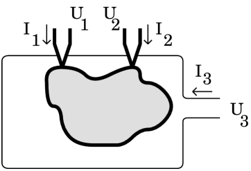
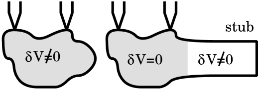
(a)                                                                                     (b)

FIG. 1.: (a) Chaotic cavity (grey), coupled to source and drain reservoir (1 and 2) by point contacts. The cavity is coupled capacitively to the gate (3). (b) Construction of the energy dependent ensemble of scattering matrices. A change $\delta\varepsilon$ of the energy is replaced by a spatially uniform change $\delta V=-\delta\varepsilon/e$ of the potential in the cavity (left), which in turn is statistically equivalent to a chaotic cavity with $\delta V=0$ (right), coupled to a closed lead (a stub) with an energy-dependent reflection matrix.

A calculation of the admittance proceeds in two steps [7]. First, we calculate the unscreened admittance $G^{u}_{\mu\nu}(\omega)$, the direct response to the change in the external potentials (at fixed internal potential)

$$G_{\mu\nu}^{u}(\omega)=\int d\varepsilon\,{f(\varepsilon-\frac{1}{2}\hbar\omega)-f(\varepsilon+\frac{1}{2}\hbar\omega)\over\hbar\omega}\mbox{tr}\,\left[\delta_{\mu\nu}\openone_{\mu}-S_{\mu\nu}^{\dagger}(\varepsilon-\frac{1}{2}\hbar\omega)S_{\mu\nu}^{\vphantom{\dagger}}(\varepsilon+\frac{1}{2}\hbar\omega)\right].$$ (2)

Here $f(\varepsilon)$ is the Fermi function, $S_{\mu\nu}$ is the $N_{\mu}\times N_{\nu}$ scattering matrix for scattering from $\nu$ to $\mu$, and $\openone_{\mu}$ is the $N_{\mu}\times N_{\mu}$ unit matrix. Second, we take the screening due to the long-range Coulomb interactions into account, which was ignored in Eq. (2). For a single self-consistent potential within the cavity, the result is [7]

$$G_{\mu\nu}(\omega) = G_{\mu\nu}^{u}(\omega)+{\sum_{\rho=1}^{2}G_{\mu\rho}^{u}(\omega)\sum_{\sigma=1\vphantom{\rho}}^{2}G_{\sigma\nu}^{u}(\omega)\over ih\omega C/2e^{2}-\sum_{\rho=1}^{2}\sum_{\sigma=1}^{2}G_{\rho\sigma}^{u}(\omega)}.$$ (3)

The average over the ensemble of quantum dots is performed using random-matrix theory [12]. We use an extension of the circular ensemble of uniformly distributed scattering matrices. This extension provides a statistical description of the energy-dependence of the scattering matrix [13]. To construct the extended circular ensemble we first replace an energy shift $\delta\varepsilon$ by a uniform decrease $\delta V=-\delta\varepsilon/e$ of the potential $V$ in the quantum dot. The key point of our method is to localize $\delta V$ in a closed lead (a stub), see Fig. 1b. The stub contains $N_{\rm s}\gg N_{1}+N_{2}$ modes to ensure that it models a spatially homogeneous potential drop $\delta V$. The system consisting of the dot and the stub is described by the $N_{\rm s}\times N_{\rm s}$, $\varepsilon$-dependent reflection matrix $r_{\rm s}(\varepsilon)$ of the stub and the $(N_{1}+N_{2}+N_{\rm s})$-dimensional scattering matrix $U$ of the cavity at reference energy $\varepsilon_{0}$, with the stub replaced by a regular open lead. We choose the scattering basis in the stub and the cavity such that $r_{\rm s}(\varepsilon_{0})=1$. For $\varepsilon$ different from $\varepsilon_{0}$ we take

$$r_{\rm s}(\varepsilon)=e^{i(\varepsilon-\varepsilon_{0})\Phi},\ \ \phi=\mbox{tr}\,\Phi$$ (4)

where the matrix $\Phi$ is Hermitian and positive definite. For $N_{\rm s}\gg N_{1}+N_{2}$, the precise choice of $\Phi$ becomes irrelevant, all information being contained in the single parameter $\phi$. For the matrix $U$ we assume a uniform distribution. In the presence of time-reversal symmetry, both $U$ and $\Phi$ are symmetric. We finally express the scattering matrix $S(\varepsilon)$ in terms of $U$ and $r_{\rm s}(\varepsilon)$,

$$S(\varepsilon) = U_{\rm ll}+U_{\rm ls}\left[1-r_{\rm s}(\varepsilon)U_{\rm ss}\right]^{-1}r_{\rm s}(\varepsilon)U_{\rm sl}.$$ (5)

The matrices $U_{ij}$ in Eq. (5) are the four blocks of $U$, describing transmission and reflection from and to the stub (s) or the two leads (l). The parameter $\phi$ is related to the mean level density $\langle dn/d\varepsilon\rangle$ via $\phi=2\pi\langle dn/d\varepsilon\rangle$.

We are now ready to calculate the average and fluctuations of the admittance. We first compute the average of the unscreened admittance $G_{\mu\nu}^{u}(\omega)$ with the help of the diagrammatic technique of Ref. [14],

$$\langle G_{\mu\nu}^{u}(\omega)\rangle = \delta_{\mu\nu}N_{\mu}-{N_{\mu}N_{\nu}\over N(1-i\omega\tau_{d})}+{(2-\beta)N_{\mu}\over\beta N(1-i\omega\tau_{d})}\left({N_{\nu}(1-2i\omega\tau_{d})\over N(1-i\omega\tau_{d})^{2}}-\delta_{\mu\nu}\right)+{\cal O}(N^{-1}),$$ (6)

where $N=N_{1}+N_{2}$ and $\tau_{d}=(h/N)\langle dn/d\varepsilon\rangle$ is the dwell time. The symmetry index $\beta=1$ ($2$) in the absence (presence) of a time-reversal-symmetry breaking magnetic field; $\beta=4$ in zero magnetic field with strong spin-orbit scattering. Since fluctuations in $G_{\mu\nu}^{u}(\omega)$ are of relative order $N^{-2}$, we may directly substitute the result (6) into Eq. (3), to obtain the first two terms in the large-$N$ expansion of the screened admittance $\langle G_{\mu\nu}(\omega)\rangle$,

$$\langle G_{\mu\nu}(\omega)\rangle = \delta_{\mu\nu}N_{\mu}-{N_{\mu}N_{\nu}\over N(1-i\omega\tau)}+{(2-\beta)N_{\mu}\over\beta N(1-i\omega\tau_{d})}\left({N_{\nu}(1-2i\omega\tau)\over N(1-i\omega\tau)^{2}}-\delta_{\mu\nu}\right)+{\cal O}(N^{-1}),$$ (7)

where $\tau^{-1}=\tau_{d}^{-1}+2e^{2}N/hC$ is the $RC$ time. The ${\cal O}(N)$ term in the r.h.s. of Eq. (7) is the classical admittance, the $\beta$-dependent ${\cal O}(1)$ term is the weak-localization correction. Notice the almost complete formal similarity between the fully screened result (7) and the unscreened result (6): Up to one term, screening results in the replacement of the dwell time $\tau_{d}$ by the $RC$-time $\tau$. The fact that the similarity is not complete is the key result of this work which we discuss below in more detail.

The first two terms in the small-$\omega$ expansion of $\langle G_{\mu\nu}(\omega)\rangle$ yield the average d.c. conductance $\langle G_{\mu\nu}\rangle$ and emittance $\langle E_{\mu\nu}\rangle$,

$$\langle G_{\mu\nu}\rangle = N_{\mu}\left(\delta_{\mu\nu}-{N_{\nu}/N}\right)+(2-\beta)({N_{\mu}/\beta N})\left({N_{\nu}/N}-\delta_{\mu\nu}\right),$$ (9)

$$\langle E_{\mu\nu}\rangle = {N_{\mu}N_{\nu}\tau/N}-(2-\beta)({N_{\mu}\tau_{d}/\beta N})\left({N_{\nu}/N}-\delta_{\mu\nu}\right).$$ (10)

Eq. (9) was previously obtained in Ref. [4]. For $C\to 0$, the $RC$-time $\tau$ vanishes. For $\beta=2$ we then find $\langle E_{\mu\nu}\rangle=0$, for $\beta=1$ the weak-localization contribution $\langle E_{11}\rangle=-\langle E_{12}\rangle=N_{1}N_{2}\langle dn/d\varepsilon\rangle/N^{3}h$ leads to a positive emittance, while for $\beta=4$ the emittance is negative. For comparison we mention that for complete screening, a ballistic conductor has an inductive emittance $E=-(1/4h)\langle dn/d\epsilon\rangle$, whereas a metallic diffusive conductor behaves capacitively as $E=(1/6h)\langle dn/d\epsilon\rangle$ [9].

For simplicity, we restrict our presentation of the admittance fluctuations to the d.c. conductance $G_{\mu\nu}$ and the emittance $E_{\mu\nu}$ at zero temperature. As before, we use the diagrammatic technique of Ref. [14]. The leading $\omega$-behavior of the admittance fluctuations is determined by the cross-correlator $\mbox{cov}\,(G_{\mu\nu},E_{\mu\nu})$ [Recall that $\mbox{cov}\,(x,y)=\langle xy\rangle-\langle x\rangle\langle y\rangle$]. We find that $\mbox{cov}\,(G_{\mu\nu},E_{\mu\nu})$ is unaffected by the capacitive interaction with the gate,

$$\mbox{cov}\,(G_{\mu\nu},E_{\rho\sigma})=\mbox{cov}\,(G_{\mu\nu},E_{\rho\sigma}^{u}) = -{N_{\mu}N_{\nu}\,\tau_{d}\over N^{2}}\left({N_{\rho}\over N}-\delta_{\mu\rho}\right)\left({N_{\sigma}\over N}-\delta_{\nu\sigma}\right).$$ (11)

For the autocorrelator of the emittance we find

$$\mbox{cov}\,(E_{\mu\nu},E_{\rho\sigma}) = {3\,N_{\mu}N_{\nu}\tau_{d}^{2}\over 2\,N^{2}}\left({N_{\rho}\over N}-\delta_{\mu\rho}\right)\left({N_{\sigma}\over N}-\delta_{\nu\sigma}\right)+{N_{\mu}N_{\nu}\tau^{2}\over N^{3}}\left(\delta_{\mu\rho}N_{\sigma}+\delta_{\nu\sigma}N_{\rho}\right)$$ (13)

$$\mbox{}+{2\,N_{\mu}N_{\nu}N_{\rho}N_{\sigma}\tau^{2}\over\tau_{d}^{2}N^{4}}(\tau^{2}-\tau_{d}^{2}).$$

Eqs. (11) and (13) are valid for $\beta=2$. In zero magnetic field ($\beta=1,4$), the permutation $\rho\leftrightarrow\sigma$ must be added; in the presence of spin-orbit scattering ($\beta=4$), Eqs. (11) and (13) are multiplied by $1/4$.

The relevant time scales for the low-frequency response of a chaotic quantum dot are obtained from Eqs. (10) and (11). The relevant time scale for the classical admittance is the charge-relaxation time $\tau$, while the weak-localization correction $\delta G_{\mu\nu}(\omega)$ and the admittance fluctuations are governed by the dwell time $\tau_{d}$. Hence, to leading order in $\omega$, the manifestation of quantum phase coherence on a.c. transport is unaffected by the Coulomb interactions. For a macroscopic quantum dot, the density of states $dn/d\varepsilon\gg C/e^{2}$, so that the two characteristic time scales $\tau$ and $\tau_{d}$ differ considerably.

To explain this result, we first consider the weak-localization correction $\delta E_{\mu\nu}$ to the average emittance. A screening contribution to $\delta E_{\mu\nu}$ requires a magnetic-field dependent quantum interference correction to the charge accumulated in the cavity. To first order in $\omega$, the (unscreened) charge accumulation at a point $\vec{r}$ in the dot due to the external potential change $\delta U_{\mu}(\omega)$ is determined by the injectivity $d\overline{n}_{\mu}(\vec{r})/d\varepsilon$ and emissivity $d\underline{n}_{\mu}(\vec{r})/d\varepsilon$ [8, 9]. For symmetry reasons, the ensemble averages $\langle d\overline{n}_{\mu}(\vec{r})/d\varepsilon\rangle$ and $\langle d\underline{n}_{\mu}(\vec{r})/d\varepsilon\rangle$ both equal $N_{\mu}/N$ times the average local density of states $\langle dn(\vec{r})/d\varepsilon\rangle$, and have no magnetic-field dependent weak-localization correction. Hence weak localization affects how current is distributed into the different leads, but it does not lead to charging of the sample (to leading order in $\omega$). This explains why the relevant time scale is the dwell time $\tau_{d}$, characteristic of the non-interacting system, and not the charge-relaxation time $\tau$.

Similarly, the screening correction to $\mbox{cov}\,(G_{\mu\nu},E_{\mu\nu})$ requires correlations between $G_{\mu\nu}$ and the injectivity $d\overline{n}_{\rho}(\vec{r})/d\varepsilon$ or emissivity $d\underline{n}_{\rho}(\vec{r})/d\varepsilon$ [8, 9]. For a chaotic cavity, we have

$$\mbox{cov}\,(G_{\mu\nu},d\overline{n}_{\rho}(\vec{r})/d\varepsilon) = \mbox{cov}\,(G_{\mu\nu},d\underline{n}_{\rho}(\vec{r})/d\varepsilon)=N_{\rho}\,\mbox{cov}\,(G_{\mu\nu},dn(\vec{r})/d\varepsilon)/N.$$ (14)

The correlator of the d.c. conductance and the local density of states vanishes for ideal leads, which is easily verified by computation of $\kappa_{ij}=\mbox{cov}\left(|S_{ij}|^{2},dn(\vec{r})/d\varepsilon\right)$. For $\beta=2$ both $dn(\vec{r})/d\varepsilon$ and the distribution of $S$ are invariant under multiplication of $S$ with a unitary matrix. It follows that $\kappa_{ij}$ is independent of $i$ and $j$, hence $\kappa_{ij}=0$. For $\beta=1,4$ a similar argument holds. The absence of correlations between the density of states and the d.c. conductance is special for the case of ideal point contacts. Correlations between $G_{\mu\nu}$ and $dn(\vec{r})/d\varepsilon$ are common for point contacts with tunnel barriers, when the scattering matrix has no uniform distribution.

The average and variance of the admittance of a chaotic quantum dot with only one point contact is obtained from our results by setting $N_{1}=N$, $N_{2}=0$. Denoting the admittance of this system by $G(\omega)=G_{11}(\omega)$, we thus obtain

$$\langle G(\omega)\rangle = {-Ni\omega\tau\over 1-i\omega\tau}+{(2-\beta)\omega^{2}\tau^{2}\over\beta(1-i\omega\tau_{d})(1-i\omega\tau)^{2}},\ \ \mbox{var}\,G(\omega)={4\tau^{4}\over\beta\tau_{d}^{2}}(i\omega)^{2}+{\cal O}(\omega^{3}).$$ (15)

Note that for a single point contact (see also Ref. [5]) the leading contribution to the variance of the admittance is proportional to $\omega^{2}$. Since the a.c. response of such a system is purely capacitive, the absence of a linear term in $\mbox{var}\,G(\omega)$ and the weak localization correction $\delta G(\omega)$ agrees with our previous result that quantum interference corrections to the low-frequency admittance of a two-probe quantum dot are unaffected by the Coulomb interactions.

In conclusion, we have calculated the average and variance of the admittance of a chaotic quantum dot which is coupled to two electron reservoirs via multichannel point contacts. The quantum dot is capacitively coupled to a gate. In the universal regime of multichannel point contacts, phase coherent a.c. transport is characterized by weak localization and admittance fluctuations. The relevant time scale for the quantum-interference effects at low frequencies $\omega$ is the dwell time $\tau_{d}$, while the classical admittance depends on the $RC$ time $\tau$. Since these two time scales differ several orders of magnitude for a macroscopic quantum dot ($\tau\ll\tau_{d}$), this effect should be clearly visible in a measurement of the a.c. response of a chaotic quantum dot.

We would like to thank the organizers of the workshop on “Quantum Chaos” at the Institute for Theoretical Physics in Santa Barbara, where this research was started. This work was supported in part by the Dutch Science Foundation NWO/FOM, the Swiss National Science Foundation, and by the NSF under Grant no. PHY94–07194.

REFERENCES

- [1] R. A. Jalabert, H. U. Baranger, and A. D. Stone, Phys. Rev. Lett. 65, 2442 (1990); H. U. Baranger, R. A. Jalabert, and A. D. Stone, Phys. Rev. Lett. 70, 3876 (1993).
- [2] V. N. Prigodin, K. B. Efetov and S. Iida, Phys. Rev. Lett. 71, 1230 (1993); K. B. Efetov, Phys. Rev. Lett. 74, 2299 (1995).
- [3] V. N. Prigodin, B. L. Altshuler, K. B. Efetov and S. Iida, Phys. Rev. Lett. 72, 546 (1994); V. N. Prigodin, K. B. Efetov and S. Iida, Phys. Rev. B 51, 17223 (1995).
- [4] H. U. Baranger and P. A. Mello, Phys. Rev. Lett. 73, 142 (1994); R. A. Jalabert, J.-L. Pichard, and C. W. J. Beenakker, Europhys. Lett. 27, 255 (1994).
- [5] V. A. Gopar, P. A. Mello, and M. Büttiker, Phys. Rev. Lett. 77, 3005 (1996).
- [6] N. Kumar and A. M. Jayannavar, preprint cond-mat/9607042.
- [7] M. Büttiker, A. Prêtre, and H. Thomas, Phys. Rev. Lett. 70, 4114 (1993).
- [8] M. Büttiker, J. Phys.: Condens. Matter 5, 9361, (1993); M. Büttiker, H. Thomas, and A. Prêtre, Z. Phys. B 94, 133 (1994).
- [9] T. Christen and M. Büttiker, Phys. Rev. Lett. 77, 143 (1996); M. Büttiker and T. Christen, in Quantum Transport in Semiconductor Submicron Structures, edited by B. Kramer, NATO ASI Series Vol. 326 (Kluwer, Dordrecht, 1996).
- [10] P. W. Anderson, E. Abrahams, and T. V. Ramakrishnan, Phys. Rev. Lett. 43, 718 (1979); L. P. Gor’kov, A. I. Larkin, and D. E. Khmel’nitskiǐ, Pis’ma Zh. Eksp. Teor. Fiz. 30, 248 (1979) [JETP Lett. 30, 228 (1979)].
- [11] B. L. Al’tshuler, Pis’ma Zh. Eksp. Teor. Fiz. 41, 530 (1985) [JETP Lett. 41, 648 (1985)]; P. A. Lee and A. D. Stone, Phys. Rev. Lett. 55, 1622 (1985).
- [12] M. L. Mehta, Random Matrices (Academic, New York, 1991).
- [13] A detailed derivation together with a proof of the equivalence with the Hamiltonian approach to chaotic scattering [J. J. M. Verbaarschot, H. A. Weidenmüller, and M. R. Zirnbauer, Phys. Rep. 129, 367 (1985)] will be published elsewhere. A similar extension of the circular ensemble to model the magnetic-field dependence of is discussed in P. W. Brouwer and C. W. J. Beenakker, Phys. Rev. B 54, 1 November 1996 (cond-mat/9607101).
- [14] P. W. Brouwer and C. W. J. Beenakker, J. Math. Phys. 37, 4904 (1996).