THE THEORY OF BOUNDARY CRITICAL PHENOMENA^†

Abstract

An introduction into the theory of boundary critical phenomena and the application of the field-theoretical renormalization group method to these is given. The emphasis is on a discussion of surface critical behavior at bulk critical points of magnets, binary alloys, and fluids. Yet a multitude of related phenomena are mentioned. The most important distinct surface universality classes that may occur for a given universality class of bulk critical behavior are described, and the respective boundary conditions of the associated field theories are discussed. The short-distance singularities of the order-parameter profile in the diverse asymptotic regimes are surveyed.

1 Introduction

Until the end of the 70ies at least the subject of boundary critical phenomena[1, 2] attracted only rather limited attention, even though a number of pioneering papers had already been written on it. This was due to several reasons. Perhaps the most important one was the complete lack of sufficiently precise experimental work. Such work even seemed beyond reach of the then available experimental possibilities. Another reason was that the powerful machinery of the field-theoretical renormalization group (RG) approach had not yet been extended to systems with boundaries, and hence could be utilized for systematic studies of boundary critical phenomena[2]${}^{\mbox{\scriptsize--\,}}$[12] only later. Finally, also the seminal work of Belavin, Polyakov, and Zamolodchikov[13] on two-dimensional conformal field theories had yet to be performed and extended to systems with surfaces.[14]

Today the situation has changed considerably. The subject has become a very active research field, attracting many scientists with a broad range of diverse backgrounds. This includes the experimental and theoretical condensed matter physicist who is interested in the critical behavior of magnets and alloys with free surfaces[1, 2, 15] just as well as the physical chemist investigating the critical adsorption of binary fluids on walls and interfaces,[16] or the theoretical high-energy physicist studying field theories on manifolds with boundaries.[17] Further, there is a wealth of related phenomena. The reader can get a first impression from the following incomplete list of topics belonging to the realm of boundary critical phenomena:

• critical behavior of magnets and alloys with free surfaces,[1, 2, 15]

• critical adsorption of fluids on walls and interfaces,[16]${}^{\mbox{\scriptsize--\,}}$[21]

• critical adsorption of polymers on walls,[22]

• percolation transitions in systems with boundaries,[23]

• quantum impurity problems (such as the Kondo effect),[24]

• Schrödinger representation in renormalizable field theories,[25]

• Casimir effect,[26]

• relaxation processes starting from initial non-equilibrium states,[27, 28]

• dynamical critical phenomena in systems with boundaries.[7, 29]${}^{\mbox{\scriptsize--\,}}$[32]

The common feature of these phenomena is that their physics on large length and time scales is described by nearly critical (or ‘massless’) field theories on manifolds with boundaries. These boundaries may be genuine surfaces [as in examples (i), (iv), (vii), (ix)], walls [as in (ii), (iii), (vii)], or interfaces separating a nearly critical phase (such as a binary mixed fluid near its consolute point) from a non-critical spectator phase (such as vapor), where the latter example applies to the case of critical adsorption (ii) of a binary fluid mixture at its critical end point.[33]${}^{\mbox{\scriptsize--\,}}$[35] In quantum impurity problems[24] [topic (v)], the role of the boundaries is played by the impurities, which turn out to be equivalent to boundary conditions of the resulting effective 1+1 dimensional field theories. In the examples (vi) and (viii) one is dealing with the time evolution from a given initial state at time $t_{i}$; here the space-time hyperplane $t=t_{i}$ is the analog of a boundary.[25, 28]

The purpose of this paper is to give a brief introduction into the field of boundary critical phenomena and to survey some recent pertinent RG results. The emphasis will be laid on a discussion of topics (i) and (ii). This also serves to explain the basic questions arising in, as well as general aspects of, boundary critical phenomena. In addition, typical theoretical strategies will be described and some representative experimental results mentioned. A detailed exposition of the other topics, (iii)–(ix), is beyond the scope of the present article. The reader should consult the cited literature for more information about these.

2 Surface effects

Owing to their conceptual simplicity, ferromagnets are a convenient starting point. In studies of bulk critical behavior, two important properties of real ferromagnets are usually ignored: their finite size and the presence of surfaces. To gain insight into the significance of these properties, consider a ferromagnet of finite linear extension $L$, where $L$ is large in comparison with the characteristic microscopic scale, the lattice constant $a$. For concreteness, we take a $d$ dimensional cube. Its $2d$ faces make up the boundary of total surface area $A=2dL^{d-1}$. We presume that the microscopic interactions are of short range. As a microscopic model one can imagine an Ising model on the lattice $[0,L]^{d}\cap Z\!\!\!\!Z^{d}$, with a Boltzmann factor $\exp(-{\cal H\/}_{\mbox{\scriptsize lat}})$ of the form

$${\cal H\/}_{\mbox{\scriptsize lat}}=\frac{1}{2}\sum_{{\mbox{\boldmath$i$}}\neq{\mbox{\boldmath$j$}}}K_{{\mbox{\boldmath$i$}}{\mbox{\boldmath$j$}}}\,s_{{\mbox{\boldmath$i$}}}\,s_{{\mbox{\boldmath$j$}}}\;.$$ (1)

Here $i$ labels the sites, and $s_{{\mbox{\boldmath$i$}}}=\pm 1$ are spin variables. Away from the surface, the interaction constants are translation invariant, $K_{{\mbox{\boldmath$i$}}{\mbox{\boldmath$j$}}}=K({\mbox{\boldmath$i$}}\!-\!{\mbox{\boldmath$j$}})$, but close to it $K_{{\mbox{\boldmath$i$}}{\mbox{\boldmath$j$}}}$ will in general also depend on the distance of the bond’s center from the surface. Restricting ourselves to nearest-neighbor (nn) interactions, we assume that $K_{{\mbox{\boldmath$i$}}{\mbox{\boldmath$j$}}}$ takes the value $K_{1}$ for all nn bonds between two surface sites, the ‘bulk value’ $K$ for all other nn bonds, and is zero otherwise. It is understood that both $K$ and $K_{1}$ are ferromagnetic $(<0)$. No restriction is imposed on the boundary variables $s_{{\mbox{\boldmath$i$}}}$ (free boundary conditions).

The presence of surfaces entails that thermal averages of local densities deviate from their values deep inside the sample. Far away from the critical point $K=K_{c}$, this disturbance can penetrate into the sample only up to a distance comparable with the interaction range, for the correlation length $\xi$ is of the same (microscopic) order. However, as the temperature $T$ approaches the bulk critical temperature $T_{c}$, $\xi$ grows, getting macroscopically large. Hence the boundary region affected by the surface acquires a thickness of the same macroscopic order. An obvious first consequence is:

• Local densities such as the order parameter $m({\mbox{\boldmath$x$}})$ or the energy density $\varepsilon({\mbox{\boldmath$x$}})$ become inhomogeneous on the scale of $\xi$.

In our case, $m({\mbox{\boldmath$x$}})$ and $\varepsilon({\mbox{\boldmath$x$}})$ correspond to (coarse-grained versions of) the local magnetization $m({\mbox{\boldmath$i$}})=\langle s_{{\mbox{\boldmath$i$}}}\rangle$ and energy

$$\varepsilon({\bf i})=\sum_{\mbox{\footnotesize nn bonds of }{\mbox{\boldmath$i$}}}\langle s_{{\mbox{\boldmath$i$}}}s_{{\mbox{\boldmath$j$}}}\rangle\;,$$ (2)

respectively.

The position-dependence of the magnetization for $T<T_{c}$ along a line perpendicular to one pair of faces, and sufficiently far away from the others, is shown schematically in Fig. 1 for the case $\xi\ll L$.

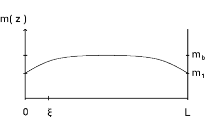
Figure 1: Schematic order-parameter profile $m(z)$ between two parallel faces, where $z$ is the distance from the left face. Up to exponentially small correction terms due to the faces not shown, the profile is independent of the coordinates perpendicular to $z$.

Deep inside the bulk, $m({\mbox{\boldmath$x$}})$ agrees with the bulk value $m_{b}$ up to corrections $\sim\exp(-z/\xi)$ (and analogous ones with $z$ replaced by the distance to the other faces). Owing to the reduced coordination number at the surface, one expects the profile to decrease upon approaching the surface provided the interactions are not too strongly enhanced near the surface. However, it is also possible that the magnetization profile bends upwards near the surface. This may happen when the enhancement of surface interactions is sufficiently strong, or when the magnetization is locally increased by a magnetic field acting only on spins in the vicinity of the surface. As we shall see later, there may even be changeovers between different asymptotic forms of large-scale behavior in the region $z\mathrel{\mathchoice{\lower 3.0pt\vbox{\halign{$\hfill#\hfil$\cr<\crcr\sim\crcr}}}{\lower 3.0pt\vbox{\halign{$\hfill#\hfil$\cr<\crcr\sim\crcr}}}{\lower 3.0pt\vbox{\halign{$\hfill#\hfil$\cr<\crcr\sim\crcr}}}{\lower 3.0pt\vbox{\halign{$\hfill#\hfil$\cr<\crcr\sim\crcr}}}}\xi$ if certain surface-related crossover lengths become much larger than the lattice constant $a$. Of course, on the scale of $a$, the behavior of the densities depends on microscopic details (chosen interactions, lattice type, etc).

A second, equally obvious, consequence is

• the appearance of surface corrections in integrated densities.

For example, the total order parameter per volume $V$ ($=L^{d}$) can be written as

$$\frac{1}{V}\int_{\cal M}\!d^{d}x\;m({\mbox{\boldmath$x$}})\approx m_{b}+\frac{A}{V}\,m_{s}+\ldots$$ (3)

in the limit $L\to\infty$. Here ${\cal M\/}$ denotes the region $\subset I\!\!R^{d}$ occupied by the system. The ellipsis stands for (edge) contributions $\sim L^{-2}$ and faster decaying ones. The quantity $m_{s}$ is called surface excess magnetization. An analogous decomposition into a bulk term, $f_{b}$, and an excess contribution $f_{s}$, called surface free energy density, holds for the reduced free energy

$${F\over k_{B}T}\equiv-\ln\mbox{Tr\,}e^{-{\cal H\/}_{\mbox{\tiny lat}}}\;$$ (4)

and other quantities.

Surface corrections like $AV^{-1}f_{s}$ are small for large $L$ as long as $\xi\ll L$. For temperatures $T$ sufficiently close to the pseudo-critical temperature[36]${}^{\mbox{\scriptsize--\,}}$[38] $T_{L}=T_{c}+O(L^{-\nu})$ of the finite system, the correlation length is of the same order as $L$. Then the separation $(\ref{bulksurf})$ into bulk and surface contributions looses its meaning. Finite-size effects become important. These have been surveyed by Dohm recently[39]. Since our subject here is boundary effects, we will always assume that $\xi\ll L$. Hence we first take the thermodynamic limit $L\to\infty$ and only then consider the approach to the critical point. By this procedure finite-size effects are eliminated. It amounts to the study of semi-infinite systems. In most of the following we will restrict our attention to these.

The critical behavior of bulk densities is described by familiar power laws. For the order parameter $m_{b}$, and the singular parts of the energy density $\varepsilon_{b}$ and free energy $f_{b}$, one has, in zero magnetic field,

$$m_{b}\approx M_{-}|\tau|^{\beta}\quad\mbox{as }\tau\to 0^{-}\,,$$ (5)

and

$$\varepsilon^{\mbox{\scriptsize(sing)}}_{b}\approx{B_{\pm}\over 1-\alpha}\,|\tau|^{1-\alpha}\;,\quad f^{\mbox{\scriptsize(sing)}}_{b}\approx B_{\pm}\,|\tau|^{2-\alpha}\quad\mbox{as }\tau\to 0^{\pm}\,,$$ (6)

respectively. Here $\alpha$ and $\beta$ are two independent standard critical exponents in terms of which all other commonly introduced bulk critical exponents can be expressed. $M_{-}$ and $B_{\pm}$ are nonuniversal (metric) factors.

It is natural to expect that local densities, taken at points within a distance $z\ll\xi$ from the surface, also display critical behavior characterized by power-law singularities, as the bulk critical point is approached. In other words, a third consequence should be

• the appearance of new critical indices characterizing the critical behavior of surface quantities.

Thus, for the local surface order parameter $m_{1}\equiv m(z\!=\!0)$, one anticipates that

$$m_{1}\sim|\tau|^{\beta_{1}}\quad\mbox{as }\tau\to 0^{-}\,,$$ (7)

where $\beta_{1}$ in general should be different from $\beta$.

This is indeed the case. It suffices here to mention just a few exemplary sources of evidence. From exact work[40] on the semi-infinite Ising model in $d=2$ dimensions it is known that $\beta_{1}=1/2$, which is to be compared with the Onsager value $\beta=1/8$. Even mean-field theory[41, 1, 2] gives different values, namely $\beta_{1}=1$ and $\beta=1/2$, independent of $d$. The first clear experimental evidence for a value of $\beta_{1}\neq\beta$, to my knowledge, is due to Alvarado et al.[42] These authors investigated the temperature dependence of $m_{1}$ at the (100) surface of a Ni ferromagnet via spin-polarized low-energy electron diffraction. They found $\beta_{1}=0.825^{+0.025}_{-0.040}\,$, a value much larger than the bulk exponent $\beta\approx 0.36$ of the three-dimensional $O(3)$ Heisenberg model, with which the observed bulk critical behavior agrees quite well. Their result for $\beta_{1}$ is in reasonable agreement with the theoretical estimate[12] $\beta_{1}(d\!=\!3,n\!=\!3)=0.84\pm 0.01$, which was obtained by combining the results of an $\epsilon=4-d$ expansion to second order[3, 43] with those of a $d-2$ expansion[12] to the same order. (Here $n$ stands for the number of components of the order parameter.)

More recently, the method of X-ray scattering under grazing incidence has been employed with impressive success to study the surface critical behavior of the binary alloy FeAl.[44, 15] As suggested in the theoretical work of Dietrich and Wagner,[45]${}^{\mbox{\scriptsize--\,}}$[47] this technique lends itself well to accurate investigations of surface critical exponents. It enables one to determine several surface critical exponents independently, so that scaling relations can be checked.

FeAl has a rather rich phase diagram.[15] The measurements of Mailänder et al[44, 15] were performed at the continuous bulk phase transition between the high-temperature phase with B2 ordering and the low-temperature phase with DO₃ ordering. This transition involves a two-component order parameter;[48] its bulk exponent $\beta$ should agree with the value $\beta(3,2)\approx 0.345$ of the $O(2)$ $|\phi|^{4}$ model in $d=3$ dimensions. This appears to be the case, although the precision of the experimental estimates is not sufficient to discriminate between the Ising value[50] $\beta_{1}(3,1)\approx 0.33$ and the one for $n=2$ given above. In any case, a much larger value of $\beta_{1}$ was found again, namely[44] $\beta_{1}=0.75\pm 0.02$. This result is close to the estimate[2] $\beta_{1}(3,2)\approx 0.8$ obtained from the $\epsilon$ expansion.[3, 43]

Monte Carlo calculations for the Ising case[51]${}^{\mbox{\scriptsize--\,}}$[53] also gave clear evidence for values of $\beta_{1}\neq\beta$.

Summing up, it may be said that there is indisputable evidence for the fact that the surface exponent $\beta_{1}$ generally is different from the bulk exponent $\beta$. However, this is only part of the story. A central element of the modern theory of bulk critical phenomena is the division into (bulk) universality classes. An obvious question to be asked is whether a similar classification can be accomplished for surface critical behavior at bulk critical points. The answer is yes. We call such classes surface universality classes. As it turns out,

• for a given bulk universality class, there exist in general several distinct surface universality classes.

To explain this we must consider specific models. Instead of continuing to work with lattice models such as the one introduced in Eq. (1), we will now turn directly to appropriate continuum models describing the large-scale physics.

3 Surface universality classes

We presume that on large scales no long-range interactions must be taken into account. This requires that the following necessary conditions are fulfilled:

• All pair interactions must be of short range or at most have long-range parts that are irrelevant in the RG sense (anywhere, i.e., both in the bulk and in the vicinity of the surface).

• All boundary-induced contributions to the interactions must be of short range in the distance $z$ from the surface or at most have parts of long range in $z$ that are irrelevant in the RG sense. This must hold, in particular, for any one-body potential associated with the boundary.

One-body potentials decaying as a power $z^{-\omega}$ as $z\to\infty$ occur in the case of fluids bounded by walls. However, the exponents $\omega$ usually are larger than the critical value $\omega_{c}=\beta/\nu$ below which such long-range tails must be expected to become relevant (see, e.g., pages 210–213 of Ref. References).

The large-scale physics of systems satisfying (I) and (II) (which the lattice model of the previous section evidently does) may be expected to be described by a continuum field theory with a local action of the form

$${\cal H\/}=\int_{\cal M}\!dV\,{\cal L\/}({\mbox{\boldmath$x$}})+\int_{\cal B}\!dA\,{\cal L\/}_{1}({\mbox{\boldmath$x$}})\;,$$ (8)

where ${\cal L\/}({\mbox{\boldmath$x$}})$ and ${\cal L\/}_{1}({\mbox{\boldmath$x$}})$ are functions of the order-parameter field $\phi({\mbox{\boldmath$x$}})$ and its derivatives. For a general $d$ dimensional manifold ${\cal M\/}$ with boundary $\partial{\cal M\/}={\cal B\/}$, the representation-invariant volume and area elements are given by[17] $dV=\sqrt{g}\,d^{d}x$ and $dA=\sqrt{g_{\cal B}\/}\,d^{d-1}x_{\|}$, respectively, where $g(\bf x)$ is the determinant of the metric tensor while $g_{\cal B\/}$ is its analog for the induced metric on ${\cal B\/}$. We will restrict ourselves to manifolds ${\cal M\/}\subset I\!\!R^{d}$ in the sequel, and unless stated otherwise, we will also not consider curved boundaries. Working with semi-infinite systems, our standard choice of ${\cal M\/}$ will be the $d$ dimensional half-space $I\!\!R^{d}_{+}\equiv\{({\mbox{\boldmath$x$}}_{\|},z)\in I\!\!R^{d}\mid 0\leq z<\infty\}$, with ${\cal B\/}$ given by the $z=0$ plane. Thus $dV$ and $dA$ can simply be read as $d^{d}x$ and $d^{d-1}x_{\|}$, respectively.

The ‘bulk density’ ${\cal L\/}({\mbox{\boldmath$x$}})$ must be chosen in such a way that a proper description of bulk critical behavior results. In the case of a usual critical point of systems belonging to the universality class of the isotropic $n$-vector model, this tells us to choose

$${\cal L\/}({\mbox{\boldmath$x$}})={\textstyle\frac{1}{2}}\left[\nabla\phi({\mbox{\boldmath$x$}})\right]^{2}+{\cal U\/}[\phi({\mbox{\boldmath$x$}})]$$ (9)

with

$${\cal U\/}(\phi)={\textstyle\frac{1}{2}}\tau_{0}\phi^{2}+{\textstyle\frac{1}{4!}}u_{0}|\phi|^{4}\;,$$ (10)

up to symmetry-breaking terms.

In the overwhelming part of the following it will not be necessary to include derivative terms in the ‘boundary density’ ${\cal L\/}_{1}$. Hence we choose it to be of the form

$${\cal L\/}_{1}({\mbox{\boldmath$x$}})={\cal U\/}_{1}[\phi({\mbox{\boldmath$x$}})]\;.$$ (11)

In fact, for the Hamiltonians representing the surface universality classes we will be concerned with, the choice

$${\cal U\/}_{1}(\phi)={\textstyle\frac{1}{2}}c_{0}\phi^{2}-h_{1,0}\,\phi$$ (12)

is general enough. To understand why no $|\phi|^{4}$ boundary term is included, one should note that the associated coupling constant would have momentum dimension $\epsilon-1$. Thus at least for sufficiently small $\epsilon=4-d$, such a term should be irrelevant. A boundary contribution of the form $\phi\partial_{n}\phi$ cannot be excluded on the basis of power counting alone since it involves a dimensionless coupling constant. However, it can be ruled out on other grounds (it is redundant).[5, 2, 54]

The phase diagram of the semi-infinite $n$-vector model defined by Eqs. (8)–(12) with $h_{1,0}=0$ is shown in Fig. 2.

Figure 2: Phase diagram of the semi-infinite $n$-vector model for $d-1>d_{*}(n)$.

The vertical axis corresponds to $\tau_{0}$; in identifying it with $T$, we have made use of the fact that $\tau_{0}$ is a linear function of $T$ near $T_{c}$. The horizontal axis corresponds to $c_{0}$, whose negative is a measure of the enhancement of the surface interactions. The variable $c$ is proportional to $c_{0}-c_{\mbox{\scriptsize sp}}$, where $c_{\mbox{\scriptsize sp}}$ is chosen such that the point Sp is located at $c=0$. The lines labeled “ordinary”, “extraordinary”, and “surface” represent continuous phase transitions that have been given these names.[41] The lines meet at a multicritical point Sp, which describes the “special” transition. The ordinary transition occurs for subcritical surface enhancement $c>0$; it is a transition from a surface-disordered (SD), bulk-disordered (BD) phase to a surface-ordered (SO), bulk-disordered phase. On lowering the temperature at fixed supercritical enhancement $c<0$, one first enters a surface-ordered, but bulk-disordered, phase at $T=T_{\mbox{\scriptsize s}}(c)$. This so-called “surface” transition is like a bulk transition of a $d-1$ dimensional system. (The bulk correlation length of the $d$ dimensional semi-infinite system remains finite on the transition line, as long as $c$ stays away from its critical value zero.) As $T$ is lowered further at fixed $c<0$, the extraordinary transition takes place.

At bulk criticality, $T=T_{c}$, we thus have three distinct types of surface transitions: the ordinary, the special, and the extraordinary one, provided $d$ exceeds their respective lower critical dimensions (lcd). The lcd of the surface, extraordinary, and special transitions is $2$ for $n=1$, but $3$ for $n>1$.This is because a SO/BD phase cannot appear (except for infinite surface enhancement), unless the surface dimension $d-1$ is larger than $d_{*}(n)=2-\delta_{n1}$. Hence, for the isotropic Heisenberg case $n=3$, only the ordinary transition remains in three dimensions. In the particular case $d-1=n=2$, a phase with quasi-long-range order at the surface is possible. This possibility will not be considered here. Note also that the limit $n\to 0$ is known to describe the adsorption of polymers on a wall.[22] For this problem an analog of the multicritical point Sp, corresponding to an adsorption threshold, exists for $d\geq 2$.

For given $d$ and $n$, each one of the above-mentioned three types of transitions of our model is characteristic of a separate surface universality class, also called ordinary, special, and extraordinary, and described by ($h_{1,0}=0$) RG fixed points

$${\cal P\/}^{*}_{\mbox{\scriptsize ord}}:\;c^{*}_{\mbox{\scriptsize ord}}=\infty\;,\qquad{\cal P\/}^{*}_{\mbox{\scriptsize sp}}:\;c^{*}_{\mbox{\scriptsize sp}}=0\;,\qquad{\cal P\/}^{*}_{\mbox{\scriptsize ex}}:\;c^{*}_{\mbox{\scriptsize ex}}=-\infty\;,$$ (13)

respectively, with the indicated fixed-point values of $c$.

Let us briefly summarize some important properties of these transitions.

3.1 The ordinary transition

At the ordinary transition there is a single relevant surface scaling field $g_{1}$, which varies $\sim h_{1,0}$ for small $h_{1,0}$. All conventionally defined surface critical exponents can be expressed in terms of its scaling index $\Delta_{1}^{\mbox{\scriptsize ord}}/\nu$ and two independent bulk exponents. For example, the critical surface pair correlation function, the singular part of the surface energy density, and $m_{1}$ behave as

$$\left\langle\phi({\mbox{\boldmath$x$}}_{\|},0)\,\phi({\bf 0},0)\right\rangle_{T=T_{c}}\sim|{\mbox{\boldmath$x$}}_{\|}|^{-(d-2+\eta_{\|})}\;,$$ (14)

$$\varepsilon_{1}^{\mbox{\scriptsize(sing)}}\approx\hat{B}_{\pm}|\tau|^{2-\alpha}\;,$$ (15)

and

$$m_{1}\approx|\tau|^{\beta_{1}^{\mbox{\tiny ord}}}\,\sigma_{\pm}(g_{1}|\tau|^{-\Delta_{1}^{\mbox{\tiny ord}}})\;,$$ (16)

with

$$\beta_{1}=\frac{\nu}{2}\,(d-2+\eta_{\|})=(d-1)\nu-\Delta_{1}\;.$$ (17)

The exponent values of $\beta_{1}$ given in the previous section all referred to the ordinary transition. The agreement of the field-theory estimates[2, 3, 5, 12, 43, 56] with those obtained by other means is quite good, though one is far away from the precision achieved in the bulk case[50] because the field-theoretical calculations have been carried out only to two-loop order so far. For the Ising case, one finds $\beta_{1}^{\mbox{\scriptsize ord}}(3,1)\approx 0.8$. Comparisons with recent Monte Carlo and other estimates may be found in Refs. References, References, and References. Experiments with binary liquid mixtures yielded the estimate[57] $\beta_{1}^{\mbox{\scriptsize ord}}=0.83\pm 0.05$. (For another recent experiment, see Ref. References.)

Since scaling laws such as (17) can be derived quite generally from the RG equations[3, 2], they must hold to any order of the $\epsilon$ expansion (and the $d-2$ expansion[12], for $n>2$). From the RG equations one can also conclude that scaling functions such as $\sigma_{\pm}$ are universal up to a fixing of scales. In the bulk case there are two nonuniversal metric factors to be fixed (“two-scale-factor universality”). Here there is one additional nonuniversal factor, associated with the relevant surface scaling field $g_{1}$. Hence we have a $(2+1)$-scale-factor universality.[9]

To explain another important property in an elementary fashion, we note that the order parameter profile takes the scaling form

$$m(z,\tau)\approx M_{-}|\tau|^{\beta}\,P(z/\xi)\quad\mbox{with}\quad P(\zeta)\approx\cases{1&as $\zeta\to\infty$,\cr p_{0}\,\zeta^{(\beta_{1}-\beta)/\nu}&as $\zeta\to 0$,\cr}$$ (18)

where the short-distance singularity of $P(\zeta)$ follows from the requirement that $m(z\ll\xi)$ has the temperature dependence $\tau^{\beta_{1}}$ of $m_{1}$. Since $\beta_{1}^{\mbox{\scriptsize ord}}>\beta$, $P(0^{+})$ vanishes. That is, the order parameter satisfies an asymptotic Dirichlet boundary condition. This argument can be generalized in a straightforward fashion to multi-point correlation functions, both for $\tau>0$ as well as for $\tau<0$. As first shown in Ref. References, the short-distance singularity $\phi_{z\to 0}\sim z^{(\beta_{1}-\beta)/\nu}$ can be systematically obtained by means of a short-distance expansion in terms of boundary operators (cf. Refs. References and References, and Sect. 4 below). Explicit results for the scaling function $P(\zeta)$ obtained by RG-improved perturbation theory to one-loop order may be found in Ref. References.

3.2 The special transition

This transition involves besides the analog of $g_{1}$, which we call $h_{1}$, a second relevant surface scaling field, $c$. One is led to scaling forms such as

$$m_{1}(\tau,c)\approx|\tau|^{\beta_{1}^{\mbox{\tiny sp}}}\psi_{\pm}(c|\tau|^{-\Phi},h_{1}|\tau|^{-\Delta^{\mbox{\tiny sp}}_{1}})\;.$$ (19)

Standard arguments based on crossover scaling imply that the crossover exponent $\Phi$ governs the behavior of the line of surface transitions near Sp, giving $[T_{\mbox{\scriptsize s}}(c)-T_{c}]/T_{c}\sim|c|^{1/\Phi}$.

In mean-field theory $\beta_{1}^{\mbox{\scriptsize sp}}=\Phi=1/2$, independent of $n$. The $\epsilon$ expansion is known to second order. Setting $\epsilon=1$ in the corresponding $O(\epsilon^{2})$ expressions gives[2] $\beta_{1}^{\mbox{\scriptsize sp}}(3,1)\approx 0.22\ldots 0.25$, in reasonable agreement with various Monte Carlo results,[51]${}^{\mbox{\scriptsize--\,}}$[53] which yielded values in the range $0.19\ldots 0.24$ (even though the error bars reported in some of these works are much smaller). The agreement is less satisfactory for $\Phi$. Earlier simulations[51] gave $\Phi(3,1)\approx 0.59$, but more recent Monte Carlo work[52] suggests a value $\mathrel{\mathchoice{\lower 3.0pt\vbox{\halign{$\hfill#\hfil$\cr<\crcr\sim\crcr}}}{\lower 3.0pt\vbox{\halign{$\hfill#\hfil$\cr<\crcr\sim\crcr}}}{\lower 3.0pt\vbox{\halign{$\hfill#\hfil$\cr<\crcr\sim\crcr}}}{\lower 3.0pt\vbox{\halign{$\hfill#\hfil$\cr<\crcr\sim\crcr}}}}0.5$. The discrepancy with the reported $\epsilon$ expansion estimate is presumably due to the unusually large $O(\epsilon^{2})$ term of $\Phi$. This view is supported by the results of a recent paper,[56] in which the massive RG approach for fixed dimension $d=3$ has been extended to semi-infinite systems. From a two-loop calculation and subsequent Padé-Borel analysis the value $\Phi(3,1)\approx 0.54$ was found. If such elaborate techniques are used to extrapolate the $\epsilon$ expansion to $d=3$, one can get down to similarly small estimates of $\Phi$. To significantly improve the accuracy of such field-theory estimates, calculations to higher loop orders are required.

The scaling form (18) of the order-parameter profile carries over to the present $c=0$ case (with $n=1$), but now the exponent $\beta_{1}^{\mbox{\scriptsize sp}}-\beta$ of the short-distance singularity is negative for $3\leq d<4$. Hence the analog of $P(\zeta)$ tends to $+\infty$ as $\zeta\to 0$. Only when $\beta_{1}^{\mbox{\scriptsize sp}}=\beta$ (as in mean-field theory and hence for $d>4$), do we have a Neumann boundary condition $\partial_{n}\phi=0$. Again, these scaling considerations can be extended to $N$-point correlation functions, and the short-distance singularities can be derived in a systematic manner via a boundary-operator expansion (cf. Sect. 4).

3.3 Extraordinary and normal transitions and critical adsorption

The special feature of the extraordinary transition is that there is spontaneous symmetry breaking and long-range surface order both below and above $T_{c}$. Bray and Moore[59] argued that the important point is just that $m_{1}$ remains nonzero at the transition. Instead of having long-range surface order caused by spontaneous symmetry breaking for $T\mathrel{\mathchoice{\lower 3.0pt\vbox{\halign{$\hfill#\hfil$\cr>\crcr\sim\crcr}}}{\lower 3.0pt\vbox{\halign{$\hfill#\hfil$\cr>\crcr\sim\crcr}}}{\lower 3.0pt\vbox{\halign{$\hfill#\hfil$\cr>\crcr\sim\crcr}}}{\lower 3.0pt\vbox{\halign{$\hfill#\hfil$\cr>\crcr\sim\crcr}}}}T_{c}$, one could as well have surface order induced by a surface magnetic field $h_{1,0}$. In other words, the surface critical behavior of the extraordinary transition (supercritical enhancement $c<0$ and $h_{1,0}=0$) should be the same as in the case of subcritical enhancement $c>0$ with $h_{1,0}>0$. Applying scaling arguments to the latter case, they predicted the behavior $m_{1}^{\mbox{\scriptsize(sing)}}\sim|\tau|^{2-\alpha}$, corresponding to $\beta_{1}^{\mbox{\scriptsize ex}}=2-\alpha$.

The case $c>0$, $h_{1,0}\neq 0$ is quite normal for bounded fluids and binary fluid mixtures in contact with a wall, since for these a surface ordering field (and other terms breaking the $Z\!\!\!\!Z_{2}$ symmetry) generically should be present even at bulk coexistence. For this reason, the transition with $h_{1,0}\neq 0$ and arbitrary $c<\infty$ has been termed “normal”.[31, 20] Thus the claim is that the extraordinary and normal transition are representative of one and the same surface universality class, provided both are possible. (Note that the l.c.d. of the normal transition is $d=2$, whereas it is $d=3$ for the $n=1$ extraordinary transition.)

In subsequent work by Burkhardt and the present author[60] it has been possible to demonstrate the extraordinary-normal equivalence for the Ising case in an exact manner. Likewise, the asymptotic behavior at the normal and extraordinary transitions,

$$m_{1}-m_{1}^{\mbox{\scriptsize(reg)}}\approx\tilde{B}_{\pm}|\tau|^{2-\alpha}$$ (20)

with

$$m_{1}^{\mbox{\scriptsize(reg)}}=m_{1,c}+A_{1}\tau+A_{2}\tau^{2}+\ldots\;,$$ (21)

is well established.[60, 61, 20] The ratios of the coefficients $B_{\pm}$, $\hat{B}_{\pm}$ and $\tilde{B}_{\pm}$ of the $|\tau|^{2-\alpha}$ singularities in Eqs. (6), (15), and (20) are all given by the same universal bulk ratio, i.e., $\tilde{B}_{+}/\tilde{B}_{-}=\hat{B}_{+}/\hat{B}_{-}=B_{+}/B_{-}.$

In the perturbative RG approach the normal-extraordinary equivalence manifests itself as follows: If $h_{1,0}>0$, then its renormalized analog, $h_{1}$, is driven to $+\infty$ under the RG flow. The variable $c$, on the other hand, tends to $\pm\infty$ or stays at zero, depending on its initial value. It turns out that the free propagator and the zero-loop profile $m(z)$ for all these cases with $h_{1}=\infty$ are given by the same expressions and identical with their analogs for $h_{1}=0$ and $c=-\infty$. Hence the respective perturbation series agree to arbitrary order. This shows that the limiting probability distributions are the same; in this sense there is just one fixed point for both transitions.

The asymptotic behavior of the order-parameter profile can be written in the scaling form (18), but with different scaling functions $P_{\pm}(\zeta)$ for $\tau\to 0^{\pm}$. These functions have been computed by means of RG-improved perturbation theory to one-loop order in $4-\epsilon$ dimensions.[61] The results, extrapolated to $d=3$, are in reasonable agreement with Monte Carlo results.[62] The short-distance behavior of the scaling functions,

$$P_{\pm}(\zeta)\begin{array}[t]{c}\approx\\ {}^{\zeta\to 0}\end{array}\zeta^{-\beta/\nu}\left[c_{\pm}+a_{1,\pm}\,\zeta^{1/\nu}+a_{2,\pm}\,\zeta^{2/\nu}+\tilde{b}_{\pm}\,\zeta^{d}+\ldots\right]\;,$$ (22)

is in conformity with the $\tau$ dependence of $m_{1}$ given in Eq. (20). The first three contributions correspond to the terms regular in $\tau$ listed in Eq. (21); the fourth one contains the $|\tau|^{2-\alpha}$ singularity. This latter term may be understood as the contribution from the component $T_{zz}$ of the stress energy tensor to the boundary operator expansion[2, 63] (BOE)

$${\phi(\mbox{\boldmath$x$})\over\langle\phi(\mbox{\boldmath$x$})\rangle_{c}}\approx\sum_{\lambda}C_{\lambda}(z)\,{\cal O}_{\cal B}^{\lambda}(\mbox{\boldmath$x$}_{\cal B})$$ (23)

of $\phi$ for $\mbox{\boldmath$x$}=(\mbox{\boldmath$x$}_{\|},z)\to\mbox{\boldmath$x$}^{\cal B}=(\mbox{\boldmath$x$}_{\|},0)$.[64] Here $\langle\phi(\mbox{\boldmath$x$})\rangle_{c}\propto z^{-\beta/\nu}$ is the critical profile. The sum runs over a complete set of boundary operators ${\cal O}_{\cal B}^{\lambda}$ with scaling exponents $\Delta_{\lambda}$. The functions $C_{\lambda}(z)$ vary $\propto z^{\Delta_{\lambda}}$ at criticality. Consistency with Eq. (22) requires that the boundary operator in (23) with the smallest scaling dimension, except the one operator 11, has $\Delta_{\lambda}=d$. This is $T_{zz}$.

To my knowledge, there is still no experimental system that has been clearly demonstrated to have supercritical surface enhancement. Thus it is fortunate that extraordinary critical behavior can be seen at normal transitions. A much studied phenomenon, which occurs at such transitions, is the critical adsorption of fluids.[16, 18]${}^{\mbox{\scriptsize--\,}}$[21] This occurs when, for example, a binary liquid mixture is brought to its bulk critical point in the presence of an external wall (e.g., container wall) or other distinct physical interface. For such a mixture, the order parameter is a composition variable. The wall usually favors one of the components, a property which translates into the presence of a surface ordering field $h_{1,0}$. Hence one gets back to our previous choice of Hamiltonian for the normal transition. One important signature of critical adsorption can be read off from Eq. (22): the composition varies as $z^{-\beta/\nu}$ for $z\ll\xi$. A second one is that the excess order parameter $m_{s}$ (corresponding to the “total amount of adsorbed order”) diverges as $\tau^{-(\nu-\beta)}$. The analytical and Monte Carlo results given in Refs. (References) and (References) have proven useful for analyzing experiments on critical adsorption. For example, values for the universal amplitude $c_{+}$ in Eq. (22) and for certain universal ratios involving integrals of $P_{\pm}$ have been extracted from experiments. These are in fair agreement with the theoretical predictions[16, 21] considering the still large error bars of both types of estimates.

4 Field theory, boundary conditions, and short-distance singularities

Since a detailed exposition of the field-theory approach to surface critical behavior may be found Ref. References, I will restrict myself here to giving a brief summary of some essential points for readers with a background in field theory. As we have seen, ‘operators’ such as $\phi(\mbox{\boldmath$x$})$ generally have different scaling dimensions for points $x$ in the interior, $\mbox{int}\,{\cal M}\equiv{\cal M}\setminus{\cal B}$, and on the boundary, ${\cal B.\/}$ For this reason we introduce separate bulk and boundary source terms, defining

$${\cal Z}[J,J_{1}]=e^{{\cal G}[J,J_{1}]}\propto\int{\cal D}\phi\,\exp\!\left[-{\cal H}+\int_{\cal M}\!dV\,J\phi+\int_{\cal B}\!dA\,J_{1}\phi\right].$$ (24)

The functional ${\cal G}$ generates the connected correlation functions $G^{(N,M)}=\langle\phi\ldots\phi\,\phi_{\cal B}\ldots\phi_{\cal B}\rangle^{\mbox{\scriptsize con}}$ of $N$ fields $\phi(\mbox{\boldmath{$x$}}_{i})$ with $\mbox{\boldmath{$x$}}_{i}\in\mbox{int}\,{\cal M}$ and $M$ fields $\phi_{\cal B}\equiv\phi(\mbox{\boldmath{$x$}}^{\cal B}_{j})$ on the boundary.

Exploiting the invariance of ${\cal Z}$ under changes $\phi\to\phi+\delta\phi$ in a standard fashion gives the ‘equations of motion’

$$J(\mbox{\boldmath$x$})=-\Delta\phi+{\cal U}^{\prime}(\phi)\;,\quad\mbox{\boldmath$x$}\in\mbox{int}\,{\cal M}\,,$$ (25)

and

$$J_{1}(\mbox{\boldmath$x$}^{\cal B})=-\partial_{n}\phi+{\cal U}_{1}^{\prime}(\phi_{\cal B})=-\partial_{n}\phi+c_{0}\phi_{\cal B}-h_{1,0}\;,\quad\mbox{\boldmath{$x$}}^{\cal B}\in{\cal B}\,,$$ (26)

where $\partial_{n}$ is the derivative along the inward normal. The resulting boundary condition for the zero-loop profile $m^{[0]}$ reads $[\partial_{z}-c_{0}]\,m^{[0]}(z\!=\!0)=-h_{1,0}$; the one for the free propagator $G=[-\Delta+U^{\prime\prime}(m^{[0]})]^{-1}(\mbox{\boldmath$x$},\mbox{\boldmath$x$}^{\prime})$ is of the Robin type,

$$\partial_{n}G\big{(}\mbox{\boldmath$x$}^{\cal B},\mbox{\boldmath$x$}^{\prime}\big{)}={\cal U}_{1}^{\prime\prime}\big{(}m^{[0]}\big{)}\,G\big{(}\mbox{\boldmath$x$}^{\cal B},\mbox{\boldmath$x$}^{\prime}\big{)}=c_{0}\,G(\mbox{\boldmath$x$}^{\cal B},\mbox{\boldmath$x$}^{\prime})\;.$$ (27)

It is well known that $G=G_{b}+G_{s}$, where $G_{b}(|\mbox{\boldmath$x$}-\mbox{\boldmath$x$}^{\prime}|)$ is its bulk analog while $G_{s}\big{(}\mbox{\boldmath$x$},\mbox{\boldmath$x$}^{\prime}\big{)}$ is an image term. The former has an integrable singularity at $\mbox{\boldmath$x$}=\mbox{\boldmath$x$}^{\prime}$, giving rise to the familiar ultraviolet (uv) bulk singularities in Feynman graphs. The latter also becomes uv singular, but only for $\mbox{\boldmath$x$}=\mbox{\boldmath$x$}^{\prime}\in{\cal B}$. This causes additional uv singularities in Feynman graphs. Owing to the local form of the primitive divergencies, they can be absorbed by local boundary counterterms. The upshot is that the required counterterms can be written as a sum $\int_{\cal M}\mbox{CT}_{b}(\mbox{\boldmath$x$})+\int_{\cal B}\mbox{CT}_{1}(\mbox{\boldmath$x$})$ of bulk and boundary contributions. Provided one can convince oneself (e.g., by power counting) that they all have the form of the interaction terms included in the action, the theory is renormalizable. In particular, our model defined by Eqs. (8)–(12) turns out to be (super-)renormalizable for $d=4$ ($d<4$). One important difference with the usual renormalization of infinite-space models should be stressed, however: in general, one-particle reducible renormalization parts may occur.[2, 4, 6, 25]

The counterterms needed to renormalize $G^{(N,M)}$ correspond to reparametrizations of the form

$$\phi=Z_{\phi}^{1/2}\phi^{\mbox{\scriptsize ren}}\;,\quad\tau_{0}=\tau_{c}+\mu^{2}Z_{\tau}\tau\;,\quad u_{0}=\mu^{\epsilon}Z_{u}u\;,$$ (28)

$$\phi_{\cal B}=[Z_{\phi}Z_{1}]^{1/2}\,(\phi_{\cal B})^{\mbox{\scriptsize ren}},\quad c_{0}=c_{\mbox{\scriptsize sp}}+\mu Z_{c}c\;,\quad h_{1,0}=\mu^{d/2}(Z_{\phi}Z_{1})^{-1/2}h_{1}\;,$$ (29)

where $\mu$ is the momentum scale. The $Z$ factors are meromorphic in $\epsilon$, provided dimensional regularization is used. In a theory regulated by a momentum cut-off $\Lambda$, one has $c_{\mbox{\scriptsize sp}}\sim\Lambda$, analogous to the familiar behavior $\tau_{c}\sim\Lambda^{2}$. For the dimensionally regulated theory in fixed dimensions $d<4$, a nonperturbative shift of the form $c_{\mbox{\scriptsize sp}}=u_{0}^{1/\epsilon}\,{\cal C}(\epsilon)$ occurs,[56] comparable to Symanzik’s mass-shift[65] $\tau_{c}=u_{0}^{2/\epsilon}\,{\cal T}(\epsilon)$.

RG equations for the renormalized functions $G^{(N,M)}_{\mbox{\scriptsize ren}}$ follow in a standard fashion and can be utilized to derive their scaling forms and the scaling relations for the exponents of the special transition. The scaling functions involve the scaling variables $c|\tau|^{-\Phi}$ and $h_{1}|\tau|^{-\Delta^{\mbox{\tiny sp}}_{1}}$. In addition to the bulk correlation length $\xi$, one has two surface-related lengths $\xi_{c}\sim c^{-\nu/\Phi}$ and $\xi_{1}\sim h_{1}^{-\nu/\Delta^{\mbox{\tiny sp}}_{1}}$ that become arbitrarily large as the multicritical point Sp is approached.

For $c>0$ and $h_{1}=0$, a crossover to a behavior characteristic of the ordinary transition occurs. The information about the latter is contained in the above-mentioned scaling functions. However, it cannot be deduced just from the RG equations of the $G^{(N,M)}_{\mbox{\scriptsize ren}}$. To extract it, the limiting behavior of their scaling functions for $c|\tau|^{-\Phi}\to\infty$ ($\xi_{c}\ll\xi$) must be known. Setting $c$ to its value $c^{*}_{\mbox{\scriptsize ord}}=\infty$ at ${\cal P}^{*}_{\mbox{\scriptsize ord}}$ does not really help because the bare and renormalized theories satisfy the Dirichlet boundary condition $\phi_{\cal B}^{\mbox{\scriptsize(ren)}}=0$ for $c_{0}=\infty$ and $c=\infty$ , respectively, so that all functions $G^{(N,M)}_{\mbox{\scriptsize(ren)}}$ with $M>0$ vanish in this case. Hence, to determine the critical behavior of these functions for $c>0$, one must move away from ${\cal P}^{*}_{\mbox{\scriptsize ord}}$, considering large but finite values of $c$. An alternative strategy is to infer the thermal singularities of local properties on ${\cal B}$ from those of their analogs for small $z>0$, with $c=\infty$. This involves knowledge about the corresponding short-distance singularities.

Fortunately, a convenient way of obtaining the required information has been found long ago.[3, 5] Using the boundary condition (26) [or (27), in perturbation theory], the operators $\phi_{\cal B}$ in $G^{(N,M)}$ may be replaced by $c_{0}^{-1}\partial_{n}\phi$. It follows that the desired critical behavior is given by the functions $G^{(N,M)}_{\infty}\equiv\langle\phi\ldots\phi\,\partial_{n}\phi\ldots\partial_{n}\phi\rangle^{\mbox{\scriptsize con}}$ with $c_{0}=\infty$.

The Dirichlet boundary condition of the regularized theory for $c_{0}=\infty$ holds even if $h_{1,0}\neq 0$, provided $h_{1,0}/c_{0}\to 0$ as $c_{0}\to\infty$. In order to retain a nonvanishing relevant surface field $g_{1}\sim h_{1,0}$, the limit $c_{0}\to\infty$ should be taken with $h_{1,\infty}\equiv c_{0}^{-1}h_{1,0}$ fixed. Noting that the term $\propto h_{1,0}$ in ${\cal H\/}$ can be rewritten as $-h_{1,\infty}\int_{\cal B\/}\partial_{n}\phi$, one sees that the relevant surface operator to which $g_{1}\sim h_{1,\infty}$ couples is $\partial_{n}\phi$.

Renormalization of the $c_{0}=\infty$ functions $G^{(N,M)}_{\infty}$ can be achieved by means of the reparametrizations

$$\partial_{n}\phi=[Z_{\phi}Z_{1,\infty}]^{1/2}\,(\partial_{n}\phi)^{\mbox{\scriptsize ren}},\quad h_{1,\infty}=\mu^{(d-2)/2}(Z_{\phi}Z_{1,\infty})^{-1/2}h_{1,\infty}^{\mbox{\scriptsize ren}}$$ (30)

and those given in Eq. (28). The implied RG equations of the renormalized functions $G^{(N,M)}_{\infty,\mbox{\scriptsize ren}}$ can be exploited in the usual manner to analyze the critical behavior at the ordinary transition.[2, 3, 5] In particular, the scaling relations for the critical exponents, and scaling forms such as (16) follow, with $h_{1,\infty}^{\mbox{\scriptsize}}$ playing the role of $g_{1}$.

We close with a brief discussion of short-distance singularities (cf. pp. 190–202 of Ref. References). Consider first the case of the special transition. We are interested in the asymptotic $z$ dependence of the functions $G^{(N,M)}_{\mbox{\scriptsize ren}}$ at criticality, $h_{1}=c=\tau=0$, as one of the $N$ off-surface points, $\mbox{\boldmath$x$}=(\mbox{\boldmath$x$}_{\|},z)$, approaches $\mbox{\boldmath$x$}^{\cal B}=(\mbox{\boldmath$x$}_{\|},0)$. The answer is provided by the BOE

$$\phi^{\mbox{\scriptsize ren}}(\mbox{\boldmath$x$})\begin{array}[t]{c}\approx\\ {}^{z\to 0}\end{array}C(z)\,(\phi_{\cal B})^{\mbox{\scriptsize ren}}(\mbox{\boldmath$x$}^{\cal B})\quad\mbox{with }C(z)\propto z^{-(\beta-\beta_{1}^{\mbox{\tiny sp}})/\nu}\;.$$ (31)

The form of $C(z)$ follows from its RG equation, implied by those of $G^{(N,M)}_{\mbox{\scriptsize ren}}$. The exponent of $z$ can be rewritten as $(\beta_{1}-\beta)/\nu=\eta_{\perp}-\eta$, using scaling laws.

The analog of this BOE for the functions $G^{(N,M)}_{\infty,\mbox{\scriptsize ren}}$ at $h_{1,\infty}^{\mbox{\scriptsize ren}}=\tau=0$ reads[5]

$$\phi^{\mbox{\scriptsize ren}}(\mbox{\boldmath$x$})\begin{array}[t]{c}\approx\\ {}^{z\to 0}\end{array}C_{\infty}(z)\,(\partial_{n}\phi)^{\mbox{\scriptsize ren}}(\mbox{\boldmath$x$}^{\cal B})\quad\mbox{with }C_{\infty}(z)\propto z^{(\beta_{1}^{\mbox{\tiny ord}}-\beta)/\nu}\;.$$ (32)

Obviously, this BOE applies equally well to the $G^{(N,0)}_{\mbox{\scriptsize ren}}$ at $c=\infty$ and $h_{1}=\tau=0$. That the leading contribution now arises from $\partial_{n}\phi$ rather than from $\phi_{\cal B}$ reflects the Dirichlet boundary condition of the renormalized theory at $c=\infty$.

As one moves away from the fixed points ${\cal P}^{*}_{\mbox{\scriptsize sp}}$ and ${\cal P}^{*}_{\mbox{\scriptsize ord}}$, permitting some relevant fields to be nonzero, the coefficient functions appearing in the operator algebra, in general, also depend on these scaling fields. Further, additional contributions may occur. Let us specifically consider what happens to the short-distance singularities of the functions $G^{(N,M)}_{\infty,\mbox{\scriptsize ren}}$ and the BOE (32) when a small surface field $h_{1,\infty}^{\mbox{\scriptsize ren}}$ is turned on. This problem was investigated and solved by Symanzik[25] in 1981. His results do not seem to have been recognized widely, especially not in the solid state community, even though they were reformulated in the language of the BOE and generalized to manifolds with curved boundaries in subsequent work.[17]

Note, first, that the analog of Eq. (26) for the $c_{0}=\infty$ functions $G^{(N,M)}_{\infty,\mbox{\scriptsize ren}}$ reads

$$J_{1,\infty}({\mbox{\boldmath$x$}}^{\cal B})=\phi_{\cal B}-h_{1,\infty}\;,$$ (33)

where $J_{1,\infty}$ is the source associated with $\partial_{n}\phi$. In the absence of $J_{1,\infty}$, this reduces to the boundary condition $\phi_{\cal B}=h_{1,\infty}$ for the regularized bare theory. (Position-dependent boundary values $\phi_{\cal B}$ can be imposed by retaining a nonzero $J_{1,\infty}$, as was actually done by Symanzik.) The naive analog of this boundary condition for the renormalized theory, $\lim_{\mbox{\boldmath$x$}\to\mbox{\boldmath$x$}^{\cal B}}\phi^{\mbox{\scriptsize ren}}=h_{1,\infty}^{\mbox{\scriptsize ren}}$, does not hold because of short-distance singularities. Instead one has (setting $\mu=1$)

$$C_{\leavevmode\hbox{\small 1\kern-3.3pt\normalsize 1}}(z)^{-1}\,\phi^{\mbox{\scriptsize ren}}(\mbox{\boldmath$x$})\begin{array}[t]{c}\longrightarrow\\ {}^{z\to 0}\end{array}h_{1,\infty}^{\mbox{\scriptsize ren}}\;,$$ (34)

where the choice $C_{\leavevmode\hbox{\small 1\kern-3.3pt\normalsize 1}}(z)=\int_{\cal B}dA\,G^{(1,1)}_{\infty,\mbox{\scriptsize ren}}(\mbox{\boldmath$x$},\mbox{\boldmath$0$})$ with $h_{1,\infty}^{\mbox{\scriptsize ren}}=0$ can be made (cf. pp. 16–17 of Ref. References). The behavior of this function at ${\cal P}^{*}_{\mbox{\scriptsize ord}}$ is well known[3, 5, 2] and follows directly from its RG equation, explicitly given in Ref. References. One finds

$$C_{\leavevmode\hbox{\small 1\kern-3.3pt\normalsize 1}}(z)\propto z^{1-\eta_{\perp}^{\mbox{\tiny ord}}}\;.$$ (35)

The exponent $1-\eta_{\perp}^{\mbox{\scriptsize ord}}=(\Delta_{1}^{\mbox{\scriptsize ord}}-\beta)/\nu$ reflects the different asymptotic scale dependencies $\sim\ell^{-\Delta_{1}^{\mbox{\tiny ord}}/\nu}$ and $\sim\ell^{\beta/\nu}$ of $h_{1,\infty}^{\mbox{\scriptsize ren}}$ and $\phi^{\mbox{\scriptsize ren}}$ in the infrared limit $\ell\to 0$.

Thus the BOE becomes[17]

$$\phi^{\mbox{\scriptsize ren}}(\mbox{\boldmath$x$})\begin{array}[t]{c}\approx\\ {}^{z\to 0}\end{array}C_{\leavevmode\hbox{\small 1\kern-3.3pt\normalsize 1}}(z)\,h_{1,\infty}^{\mbox{\scriptsize ren}}+C_{\infty}(z)\,(\partial_{n}\phi)^{\mbox{\scriptsize ren}}(\mbox{\boldmath$x$}^{\cal B})+\ldots\;,$$ (36)

where the ellipsis stands for less singular contributions (arising from other boundary operators as well as from the omitted additional dependence of coefficient functions such as $C_{\leavevmode\hbox{\small 1\kern-3.3pt\normalsize 1}}$ and $C_{\infty}$ on the scaling variable $h_{1,\infty}^{\mbox{\scriptsize ren}}\,z^{\Delta_{1}^{\mbox{\tiny ord}}/\nu}$.)

The existence of the short-distance singularity (36) is a central issue of a recent Letter,[66] in which it is verified by means of Monte Carlo simulations for the $d=3$ Ising case. In subsequent work by the same authors the $d=2$ Ising case is studied.[66]

The information acquired about short-distance singularities can be utilized to predict the position dependence of the order-parameter profile $m(z)\equiv\langle\phi\rangle$ in various asymptotic regimes with $z\ll\xi$. At bulk criticality, $\tau=0$, the scaling form of the profile, $m\equiv m_{c}$, reduces to[67, 2]

$$m(z)\approx z^{-\beta/\nu}\,F\big{(}zh_{1}^{\nu/\Delta_{1}^{\mbox{\tiny sp}}},ch_{1}^{-\Phi/\Delta_{1}^{\mbox{\tiny sp}}}\big{)}\;.$$ (37)

The limits $F(\infty,z_{2})$ and $F(z_{1},0)$ of the scaling function $F(z_{1},z_{2})$ must exist and be nonzero. Further, we know from the BOE (31) that $F(z_{1},0)\sim z_{1}^{\beta_{1}^{\mbox{\tiny sp}}/\nu}$ as $z_{1}\to 0$. Consistency with the scaling form near ${\cal P}^{*}_{\mbox{\scriptsize ord}}$ requires that

$$F\big{(}z_{1}\!=\!zh_{1}^{\nu/\Delta_{1}^{\mbox{\tiny sp}}},z_{2}\!=\!ch_{1}^{-\Phi/\Delta_{1}^{\mbox{\tiny sp}}}\big{)}\begin{array}[t]{c}\sim\\ {}^{z_{2}\to\infty}\end{array}W\big{(}zg_{1}^{\nu/\Delta_{1}^{\mbox{\tiny ord}}}\big{)}$$ (38)

with[2]

$$g_{1}=h_{1}c^{-y}\;,\quad y={\Delta_{1}^{\mbox{\tiny sp}}-\Delta_{1}^{\mbox{\tiny ord}}\over\Phi}={\gamma_{11}^{\mbox{\tiny sp}}-\gamma_{11}^{\mbox{\tiny ord}}\over 2\Phi}\;,$$ (39)

where we know from Eqs. (35) and (36) that $W(z_{3})\sim z_{3}^{1-\eta_{\perp}^{\mbox{\tiny ord}}}$ as $z_{3}\to 0$. In the scaling regime where Eq. (37) holds (small $c$ and $h_{1}$), both lengths $\xi_{c}\sim c^{-\nu/\Phi}$ and $\xi_{1}\sim h_{1}^{-\nu/\Delta^{\mbox{\tiny sp}}_{1}}$ are large. Eq. (38) involves a length $\xi_{\mbox{\scriptsize ord}}\sim g_{1}^{-\nu/\Delta_{1}^{\mbox{\tiny ord}}}$, which can be large or small. The resulting power laws describing the $z$ dependence of $m_{c}(z)$ in the various regimes are

$$m_{c}(z)\sim\cases{z^{-(\beta-\beta^{\mbox{\tiny sp}}_{1})/\nu}&for $z\ll\xi_{c}\;,\;\xi_{1}\;,\;\xi_{\mbox{\scriptsize ord}}$\,,\cr z^{1-\eta_{\perp}^{\mbox{\tiny ord}}}&for $\xi_{c}\ll z\ll\xi_{\mbox{\scriptsize ord}}$\,,\cr z^{-\beta/\nu}&for $\xi_{c}\ll\xi_{\mbox{\scriptsize ord}}\ll z$\,.\cr}$$ (40)

These findings are in conformity with unpublished one-loop results for $m_{c}(z)$, obtained some time ago by Ciach and myself.[68] Details can be found in a recent paper by Ciach and Ritschel.[68]

5 Concluding remarks

As I have tried to illustrate in this talk by discussing prototypical examples of such phenomena, the application of field-theoretical RG methods to the study of boundary critical phenomena is well established. It has led to deep insights, has provided a reliable theoretical framework, and yielded predictions for experimentally accessible quantities. Research over the past two decades has revealed a surprising wealth of such phenomena.

It is particularly encouraging to see that the number of experiments devoted to careful investigations of boundary critical phenomena has been constantly increasing for some years. Since more precise experimental data should be available soon, an obvious challenge for theorists is to improve the still rather moderate accuracy of the field-theoretical predictions. To this end, it would be very desirable to extend the presently available two-loop results for the $\epsilon$ expansion[2] and the massive RG approach in fixed dimensions[56] $d<4$ to higher orders, so that more precise field-theoretical estimates for critical exponents and amplitude ratios can be gained via Padé-Borel resummation techniques.

While achieving greater accuracy is certainly one important goal for future research, it should also be emphasized that only relatively few models for boundary critical phenomena have been thoroughly investigated so far. Thus interesting new features may still have to be discovered.

To illustrate this point, let me finish by reporting a result established recently.[69, 70] As we have seen above, systems exhibiting boundary critical behavior at bulk critical points also can be divided into universality classes. These surface universality classes depend on the bulk universality class and additional relevant surface properties. Examples of the latter we have come to know so far are: the short range of the change of interactions caused by the surface; their short-range nature; whether the surface enhancement is subcritical, critical, or supercritical; and whether symmetry-breaking surface terms (with $h_{1,0}\neq 0$) are present or not.

In the case of antiferromagnets in a magnetic field (sufficiently weak so that the bulk transition remains continuous) and binary alloys with non-ideal stoichiometry and a continuous order-disorder bulk transition, it turns out that the surface universality class in general also depends on the orientation of the surface plane with respect to the crystal axes. There exist both orientations that preserve, as well as those that break, the symmetry with respect to the two types of sublattices.[71] Depending on whether the orientation is symmetry preserving or breaking, ordinary and normal transitions (corresponding to the ordinary and extraordinary universality classes) are expected to occur, respectively (provided the enhancement is subcritical, which seems reasonable to assume).[69, 70] To appreciate this result one should note that, on the level of a lattice description, no ordering bulk and surface fields are present, because these would correspond to staggered magnetic fields, in antiferromagnetic language. It should be possible to check these predictions by means of experimental studies of the continuous A2–B2 bulk transitions in binary alloys such as FeCo or FeAl.

Note added in proof

We mentioned above the result taken from Ref. [48] that the disorder-order transition of FeAl from the B2 to the DO₃ phase should belong to the universality class of the O(2) $|\phi|^{4}$ model. Recently R. Leidl (U. Essen, unpublished) has reanalyzed the problem within Landau theory. He found that the Landau theory allows quadratic anisotropies. These are relevant and should drive the system to the the $n=1$ (Ising) fixed point. Thus the transition should belong to the universality class of the one-component $|\phi|^{4}$ model. Upon contacting Prof. Binder’s group we learned that similar conclusions have been reached in the paper by W. Helbing, B. Dünweg, K. Binder and D. P. Landau, Z. Physik B 80, 401 (1990), which corrects an earlier one by B. Dünweg and K. Binder, Phys. Rev. B 36, 6935 (1987) whose different conclusions are described in Ref. 48. We are grateful to Prof. Binder and B. Dünweg for kindly informing us about this matter.

References

References

- [1] For a general review of critical behavior at surfaces, see K. Binder, in Phase Transitions and Critical Phenomena, edited by C. Domb and J. L. Lebowitz (Academic Press, London, 1983), Vol. 8, pp. 1–144, and Ref. References.
- [2] For background on the field-theory approach to boundary critical behavior, see H. W. Diehl, in Phase Transitions and Critical Phenomena, edited by C. Domb and J. L. Lebowitz (Academic Press, London, 1986), Vol. 10, pp. 75–267.
- [3] H. W. Diehl and S. Dietrich, Phys. Lett. 80A, 408 (1980).
- [4] H. W. Diehl and S. Dietrich, Phys. Rev. B 24, 2878 (1981).
- [5] H. W. Diehl and S. Dietrich, Z. Phys. B 42, 65 (1981); 43, 281(E) (1981).
- [6] H. W. Diehl and S. Dietrich, Z. Phys. B 50, 117 (1983).
- [7] S. Dietrich and H. W. Diehl, Z. Phys. B 51, 343 (1983).
- [8] H. W. Diehl, S. Dietrich, and E. Eisenriegler, Phys. Rev. B 27, 2937 (1983).
- [9] H. W. Diehl, G. Gompper, and W. Speth, Phys. Rev. B 31, 5841 (1985).
- [10] H. W. Diehl and E. Eisenriegler, Europhys. Lett. 4, 709 (1987).
- [11] E. Eisenriegler and H. W. Diehl, Phys. Rev. B 37, 5257 (1988).
- [12] H. W. Diehl and A. Nüsser, Phys. Rev. Lett. 56, 2834 (1986).
- [13] A. A. Belavin, A. M. Polyakov, and A. B. Zamalodchikov, Nucl. Phys. B 241, 333 (1984).
- [14] J. L. Cardy, Nucl. Phys. B 240, 514 (1984).
- [15] For a review of experimental work, see H. Dosch, Critical Phenomena at Surfaces and Interfaces, Vol. 126 of Springer Tracts in Modern Physics (Springer, Berlin, 1992).
- [16] B. M. Law, Ber. Bunsenges. Phys. Chem. 98, 472 (1994); D. S. P. Smith and B. M. Law, Phys. Rev. E 52, 580 (1995).
- [17] D. M. McAvity and H. Osborn, Nucl. Phys. B 394, 728 (1992).
- [18] M. E. Fisher and P.-G. de Gennes, C. R. Acad. Sci. Paris Série B 287, 207 (1978).
- [19] A. J. Liu and M. E. Fisher, Phys. Rev. A 40, 7202 (1989).
- [20] H. W. Diehl, Ber. Bunsenges. Phys. Chem. 98, 466 (1994).
- [21] G. Flöter and S. Dietrich, Z. Phys. B 97, 213 (1995).
- [22] For background and references on polymer adsorption, see E. Eisenriegler, Polymers Near Surfaces (World Scientific, Singapore, 1993).
- [23] H. W. Diehl and P. M. Lam, Z. Phys. B 74, 395 (1989).
- [24] For background and references on quantum impurity problems, see P. Fendley, A. W. W. Ludwig, and H. Saleur, in STATPHYS 19, edited by H. Bailin (World Scientific, Singapore, 1995), pp. 137–157.
- [25] K. Symanzik, Nucl. Phys. B 190, 1 (1981).
- [26] M. Krech, Casimir Effect in Critical Systems (World Scientific, Singapore, 1994).
- [27] H. K. Janssen, B. Schaub, and B. Schmittmann, Z. Phys. B 73, 539 (1989).
- [28] H. K. Janssen, in From Phase Transitions to Chaos, edited by G. Györgyi, I. Kondor, L. Sasvari, and T. Tel (World Scientific, Singapore, 1992), pp. 68–91.
- [29] H. W. Diehl and S. Dietrich, in Festkörperprobleme, Vol. XXV of Advances in Solid State Physics, edited by P. Grosse (Vieweg, Braunschweig, 1985), pp. 39–52.
- [30] H. W. Diehl and H. K. Janssen, Phys. Rev. A 45, 7145 (1992).
- [31] H. W. Diehl, Phys. Rev. B 49, 2846 (1994).
- [32] F. Wichmann and H. W. Diehl, Z. Phys. B 97, 251 (1995).
- [33] B. Widom, J. Chem. Phys. 67, 872 (1977).
- [34] M. E. Fisher and P. J. Upton, Phys. Rev. Lett. 65, 2402 (1990).
- [35] M. E. Fisher and P. J. Upton, Phys. Rev. Lett. 65, 3405 (1990).
- [36] M. E. Fisher, in Critical Phenomena, Proceedings of the 51st. Enrico Summer School, Varenna, Italy, edited by M. S. Green (Academic Press, London, 1971), pp. 73–98.
- [37] M. N. Barber, in Phase Transitions and Critical Phenomena, edited by C. Domb and J. L. Lebowitz (Academic Press, London, 1983), Vol. 8, pp. 145–266.
- [38] K. Binder, Ferroelectrics 73, 43 (1987).
- [39] V. Dohm, in Proceedings of the International Conference RG96 (to be published).
- [40] B. M. McCoy and T. T. Wu, The Two Dimensional Ising Model (Harvard University Press, Cambridge, MA, 1973).
- [41] T. C. Lubensky and M. H. Rubin, Phys. Rev. B 12, 3885 (1975).
- [42] S. F. Alvarado, M. Campagna, and H. Hopster, Phys. Rev. Lett. 48, 51 (1982).
- [43] J. S. Reeve and A. J. Guttmann, Phys. Rev. Lett. 45, 1581 (1980).
- [44] X. Mailänder, H. Dosch, J. Peisl, and R. L. Johnson, Phys. Rev. Lett. 64, 2527 (1990).
- [45] S. Dietrich and H. Wagner, Phys. Rev. Lett. 51, 1469 (1983).
- [46] S. Dietrich and H. Wagner, Z. Phys. B 56, 207 (1984).
- [47] S. Dietrich and A. Haase, Phys. Rep. 260, 1 (1995).
- [48] K. Binder, in Phase Transformations in Materials, Vol. 5 of Materials Science and Technology, edited by R. W. Cahn, P. Haasen, and E. J. Kramer (VCH Verlagsgesellschaft mbH, Weinheim, 1991), pp. 143–212.
- [49] A. Aharaony, in Phase Transitions and Critical Phenomena, edited by C. Domb and M. S. Green (Academic Press, London, 1976), pp. 394–406.
- [50] J. Zinn-Justin, in Quantum Field Theory and Critical Phenomena, International series of monographs on physics (Clarendon Press, Oxford, 1989), Chap. 25, pp. 618–621.
- [51] D. P. Landau and K. Binder, Phys. Rev. B 41, 4633 (1990); K. Binder and D. P. Landau, Phys. Rev. Lett. 52, 3 (1984).
- [52] C. Ruge and F. Wagner, Phys. Rev. B 52, 4209 (1995); C. Ruge, S. Dunkelmann, and F. Wagner, Phys. Rev. Lett. 69, 2465 (1992).
- [53] U. Ritschel and P. Czerner, Phys. Rev. Lett. 75, 3882 (1995).
- [54] H. W. Diehl and A. Ciach, Phys. Rev. B 44, 6642 (1991).
- [55] H. W. Diehl and E. Eisenriegler, Phys. Rev. B 30, 300 (1984).
- [56] H. W. Diehl and M. Shpot, Phys. Rev. Lett. 73, 3431 (1994), and to be published.
- [57] L. Sigl and W. Fenzl, Phys. Rev. Lett. 57, 2191 (1986).
- [58] B. Burandt, W. Press, and S. Haussühl, Phys. Rev. Lett. 71, 1188 (1993).
- [59] A. J. Bray and M. A. Moore, J. Phys. A 10, 1927 (1977).
- [60] T. W. Burkhardt and H. W. Diehl, Phys. Rev. B 50, 3894 (1994); see also T. W. Burkhardt and J. L. Cardy, J. Phys. A 20, L233 (1987).
- [61] H. W. Diehl and M. Smock, Phys. Rev. B 47, 5841 (1993); 48, 6740(E) (1993).
- [62] M. Smock, H. W. Diehl, and D. P. Landau, Ber. Bunsenges. Phys. Chem. 98, 486 (1994).
- [63] D. M. McAvity and H. Osborn, Nucl. Phys. B 406, 655 (1993); 455, 522 (1995)
- [64] E. Eisenriegler and M. Stapper, Phys. Rev. B 50, 10009 (1994); J. L. Cardy, Phys. Rev. Lett. 65, 1443 (1990).
- [65] K. Symanzik, Lett. Nuovo Cimento 8, 771 (1973).
- [66] U. Ritschel and P. Czerner, Phys. Rev. Lett. 77, 3645; P. Czerner and U. Ritschel, Physica A 237, 240 (1996), and to be published.
- [67] E. Brézin and S. Leibler, Phys. Rev. B 27, 594 (1983).
- [68] A. Ciach, private communication, and A. Ciach and U. Ritschel, Nucl. Phys. B 489, 653 (1997).
- [69] A. Drewitz, R. Leidl, T. W. Burkhardt and H. W. Diehl, Phys. Rev. Lett. 78, 1090 (1997), preprint cond-mat/9609245 (1996).
- [70] R. Leidl and H. W. Diehl, Phys. Rev. B, to appear, preprint cond-mat/9707345; R. Leidl, A. Drewitz and H. W. Diehl, Int. J. of Thermophys., to appear, preprint cond-mat/9704215.
- [71] For earlier work on this matter, see F. Schmidt, Z. Phys. B 91, 77 (1993).
- [72] S. Krimmel, W. Donner, B. Nickel, H. Dosch, C. Sutter and G. Grübel, Phys. Rev. Lett. 78, 3880 (1997).