Dynamic Critical Phenomena in Channel Flow

Abstract

A simple model of the driven motion of interacting particles in a two dimensional random medium is analyzed, focusing on the critical behavior near to the threshold that separates a static phase from a flowing phase with a steady-state current. The critical behavior is found to be surprisingly robust, being independent of whether the driving force is increased suddenly or adiabatically. Just above threshold, the flow is concentrated on a sparse network of channels, but the time scale for convergence to this fixed network diverges with a larger exponent that that for convergence of the current density to its steady-state value. This is argued to be caused by the “dangerous irrelevance” of dynamic particle collisions at the critical point. Possible applications to vortex motion near to the critical current in dirty thin film superconductors are discussed briefly.

I Introduction

Vortices in superconductors that are driven by an applied electric current and pinned by disorder exhibit a wide range of interesting behavior. These are examples of non-linear transport in random media which is collective in that the interactions between the transported can roughly be divided into two classes: “elastic” and “plastic” depending on whether or not the interactions between the transported particles are strong enough to maintain the particles in an extended elastic structure as they move. Our interest here is plastic flow where the interactions between the particles and the random medium (“pinning”) are strong enough to break up any elastic structure. We will focus on the very strong pinning limit for which “channel flow” can occur: where the flow is not only plastic but dominated by particles moving along a sparse network of persistent channels.

Plastic flow of vortices has attracted a lot of recent interest.[1, 2] A number of experimental measurements in $2\mbox{H}$-$\mbox{NbSe}_{2}$ have been attributed to plastic flow, including an unexpected dip in the electrical resistance just below $H_{c2}$ (“peak effect”),[3, 4] anomalous $I$-$V$ curves,[5] generation of unusual broadband noise,[6] small angle neutron scattering measurements,[7] and fingerprint phenomena where the detailed shape of the $I$-$V$ curve is repeatable for a single sample but differs between samples.[8] Similar phenomena have recently been observed in two-dimensional amorphous $\mbox{Mo}_{77}\mbox{Ge}_{23}$ films [9] which are supported by numerical simulations for two-dimensional systems[10, 11, 12, 13, 14] which clearly see vortex motion dominated by flow along narrow “filamentary” channels. In addition to this indirect evidence, realtime images of moving vortices in thin films have been recorded.[15, 16, 17, 2] which clearly show individual vortices moving along narrow paths of least resistance.

Some of these experiments also suggest that in the regimes studied plastic flow only persists for forces just above the threshold for the onset of motion, i.e., near the critical current. At higher current the vortex lattice appears to become more ordered. Previous theoretical work[18, 19] that studied plastic flow has primarily concentrated on the ordering and break up of an elastic lattice by the randomness, concluding that, at least for small driving forces in two dimensions, the lattice will always break up and the flow will become plastic. Here we take a complementary approach that considers the extreme limit of a fully plastic state with only hard-core intervortex interactions.

In this paper we extend work on a simple model[20, 21] —roughly of point vortices in a thin film. It exhibits two phases: if the driving force is small the vortices are all trapped and there is no steady-state current, but if the force exceeds a finite threshold the vortices move in a static channel network whose configuration is determined by the pinning in the sample. In the steady-state just above threshold, the channels are far apart but each channel carries a high vortex current density.

We focus on the dynamic critical behavior near threshold and on the development of the channel network above threshold. This study will be primarily numerical aided by scaling analysis. The critical behavior appears to represent a universality class of non-equilibrium “phase” transitions that probably also includes some aspects of a continuum fluid model studied by Narayan and Fisher.[20]

A Outline

In the rest of the Introduction we briefly explain the model system we have investigated and then outline our main results. In Sec. II we provide a more detailed description of the model. The dynamic critical phenomena and scaling properties are explained in Sec. III, while the development of the channel network is studied in Sec. IV. Finally we compare our results to related work and consider possible applications in Sec. V.

B Model

The model studied here was introduced in Ref. [21] (where it was called the “one-deep” model). We briefly summarize its features here and define it in more detail in Sec. II.

This simple model for the motion of vortices in a two-dimensional random medium, treats the vortices as point particles with a hard-core interaction which move on a lattice. The randomness is represented by each site’s capacity to trap arriving particles and by the existence of a locally preferred direction—the “primary outlet”—for motion out of each site (see Fig. 1). The local capacity and preferred direction can be thought of as barriers for a particle to leave by one of the site’s outlets. Particles only leave through a particular outlet of a site when the number of particles present exceeds the barrier height. Increasing the driving force ($F$) corresponds to lowering all of the barrier heights which causes some sites to overflow thereby releasing particles. If one excess particle is present on a site, it always leaves thought the primary outlet. If more than one excess particle is present, one will leave through each outlet—a “split”. Decreasing the force raises barriers, creating more traps and increasing the capacity of existing traps.

Various possible histories of the system are represented by the way in which the force is changed, in this paper we will mainly consider increasing the force very quickly (“sudden” forcing) and then waiting for the particles to reach a steady-state. But we will also investigate what happens when the force is increased very slowly (“adiabatic” forcing) for comparison.

C Dynamic critical behavior

The behavior of the system is divided into two phases: A flowing phase where a steady-state current flows and a static phase with no current. In the static phase, the system has two types of sites: saturated sites at which any additional particle would overflow, and unsaturated sites or “traps”. In the static phase, the particles will respond to a sudden increase in the force only in a transient manner, with some fraction of the particles moving varying distances downhill before being trapped at previously unsaturated sites. The static configuration can be probed by adding a single particle, which, if it is added to a saturated site, will flow through primary outlets down a “drainage tree” until it stops at the unsaturated site at the bottom of the tree. At a critical force $F_{c}$, the lengths of some of the trees will diverge and above the critical force the system will have steady-state flow. A fundamental property of our model is that at large times above threshold the particle flow converges to a fixed channel network with each channel carrying its maximum capacity.[21] This implies that there are three types of lattice sites in the steady-state: network sites that carry moving particles, and off-network sites with no particle flow which can be either in the drainage basin (sites that drain to the channel network), or in finite drainage trees. The network sites form persistent channels that drain the system. The channels can join and split as they move through the system. In an infinite system, which sites are on the network (for a particular current) depends only on which outlets are the primary outlets and not on the initial particle placements.

We now summarize the critical behavior. In the flowing phase in a large system the steady-state current density (i.e., the mean number of particles per lattice site), after a sudden increase in the force to a final value of $F$ just above $F_{c}$, is found to be

$$J\sim(F-F_{c})^{\beta}.$$ (1)

Another quantity of interest in the flowing phase is the fraction of sites in the drainage basin, i.e., sites to which an added particle, following primary outlets, would continue to move indefinitely and become part of the steady-state current. The fraction of sites in the basin is found to increase as

$$B\sim(F-F_{c})^{\Gamma}.$$ (2)

Typical results from a set of simulations showing this behavior are shown in Fig. 2.

Numerical simulations of the model yield values of these exponents

$$\beta = 1.53\pm 0.03,$$ (3)

$$\Gamma = 0.49\pm 0.02.$$ (4)

These error bars, and all uncertainties quoted and plotted here, are estimates of statistical 1-$\sigma$ errors. More details of the accuracy and independence of these measurements are given in Sec. III.

1 Length scales

We are, of course, primarily interested in the behavior of infinite systems. But numerical studies of a range of system sizes yield both ways to extrapolate to infinite systems and information on the characteristic length scales in the system. Our scaling is anisotropic in the two directions, we will generally measure length ($L$) in the downhill direction and widths ($W$) in the horizontal direction.

The behavior of a finite system of length $L$ is controlled by a correlation length $\xi_{f}(F)$ as described in Sec. III. This length scale controls the finite size scaling and is found to diverge with an exponent $\nu$ as $F\rightarrow F_{c}$. In order to obtain the critical force and the correlation length it is convenient to work with $\Pi(L,W,F)$ defined as the probability that there is a steady-state current for a system of length $L$ and width $W$ at force $F$. Using the scaling of $\Pi$ we find

$$\nu=1.62\pm 0.04$$ (5)

on both sides of the threshold.

Below threshold at long times all particles are at rest and the sites can be designated saturated and unsaturated (“traps”) depending on whether an added particle will flow out of the site. The saturated sites and their primary outlets (see Fig. 3) form connected drainage trees such that an excess particle added to a site on a drainage tree comes to rest on the unsaturated terminus site at the bottom of the tree. The only important length scale is the characteristic tree length above which trees are exponentially unlikely, this we identify as proportional to $\xi_{f}$.

However, above threshold the situation is rather more complicated: there are two length scales present in the channel network. The characteristic vertical distance scale of the channel network backbone, $\xi_{n}$, which, as shown in Ref. [21], diverges as

$$\xi_{n}\sim\frac{1}{J^{2}}$$ (6)

as $J\rightarrow 0$; and the length which controls finite size scaling ($\xi_{f}$). If $\xi_{n}$ was identified with $\xi_{f}$ then we would expect $\nu=2\beta$ which is clearly ruled our by the data; instead we find $\beta/\nu=0.96\pm 0.02$. Nevertheless, $\xi_{n}$ definitely controls various physical quantities which suggests that both lengths are important above threshold.

The presence of two different correlation lengths above threshold is rather unusual (although it has appeared in other non-equilibrium dynamics critical points, for example sliding charge density waves.[22]) In our system the two lengths control two different equilibration processes. The decay of current transients is rapid with characteristic time $\xi_{f}$, however redistribution of the current to the steady-state channel network is much slower. The convergence to a fixed channel network can be seen by studying the distribution of time-averaged local currents through different sites of the lattice. For large systems at long times most of the sites either always contain moving particles or never contain moving particles. This distribution has been studied numerically and is is indeed found to converge to two delta functions (at currents of zero and one) as the system size increases with characteristic time scale of order $\xi_{n}$ and a power law tail ($1/t^{1/4}$) at long times. Because this approach to a steady-state pattern is so slow near threshold (and $\xi_{n}\gg\xi_{f}$) experiments or simulations may not reach the steady-state of the current network even if the current itself does reach its steady-state value.

The forcing in our model is strongly anisotropic and particles move much further parallel to the force (downhill) than perpendicular to it. The correlation lengths $\xi_{f}$ and $\xi_{n}$ are defined parallel to the force. For perpendicular (horizontal) distances we define two characteristic lengths $\xi_{f_{\perp}}$ and $\xi_{n_{\perp}}$ which we expect to behave as

$$\xi_{f_{\perp}}\sim\xi_{f}^{\alpha}$$ (7)

and

$$\xi_{n_{\perp}}\sim\xi_{n}^{\alpha_{n}}.$$ (8)

From Ref. [21], the properties of the channel network fix

$$\alpha_{n}=\frac{1}{2}.$$ (9)

Numerically, we obtain

$$\alpha=0.50\pm 0.05.$$ (10)

2 Adiabatic forcing and universality class

Our model seems to represent a new universality class. Some of its characteristics are reminiscent of directed invasion percolation but the behavior is qualitatively different. An important feature of directed invasion percolation[23] is that a local advance of “fluid” is not retarded by any elastic interaction with the rest of the fluid (unlike in models with elasticity representing surface tension). Our model goes further because the advancement of a local structure ahead of the rest of the particles is actively favored: as the bottom of a drainage tree moves down it collects more particles from above and hence is more likely to advance further under the “weight” of particles from above.

The exponents $\nu$, $\alpha$ and $\Gamma$ have direct analogs in directed percolation, where they take the values[24]

$$\nu_{\text{dir-perc}} \approx 1.73$$ (11)

$$\alpha_{\text{dir-perc}} \approx 0.63$$ (12)

$$\beta_{\text{dir-perc}} \approx 0.28$$ (13)

with $\beta_{\text{dir-perc}}$ analogous to our $\Gamma$. These are significantly different from our values. Indeed, even in mean field theory, which has only been analyzable for adiabatic forcing below threshold, our system is already different from directed percolation.

An important question in investigating a new class of critical phenomena is how many independent exponents there are. We will argue that the scaling exponents of the current density and of the drainage basin should be related,

$$\beta=1+\Gamma.$$ (14)

If in fact this is an equality, as is supported by the numerics and analytic arguments, then there would be only three independent exponents ($\beta$, $\nu$ and $\alpha$) as for directed percolation. In fact, we will argue that the exponent $\alpha$ should be exactly given by

$$\alpha=\frac{1}{2},$$ (15)

(consistent with the numerics) which would imply only two independent exponents in our system. These issues are closely tied to the relationship between the behavior with adiabatic versus sudden forcing.

With adiabatic forcing only one particle moves at a time when the system is below threshold. This means that there are no particle collisions—i.e., two particles never arrive at a site at the same time—and all particles move through primary outlets, i.e., there are no splits below threshold. In contrast, for sudden forcing many particles are released at once and then move down the lattice until they find traps. Even below threshold (where there is no steady-state current) there will be a transient flow with many collisions between particles. These collisions cause particles to use secondary outlets and explore sites which would otherwise not have been reached. This means extra traps are found and the threshold force is increased. Indeed we find (Sec.III B) critical forces for the two cases that are quite close but clearly different. But a more subtle question is whether the collisions change the universality class.

If the only effect of the collisions is for a finite fraction of the transient moving particles to move along different outlets then the type of forcing should not effect the universality class, as argued in Sec. III F. For adiabatic forcing the scaling relation

$$\beta_{a}=1+\Gamma_{a},$$ (16)

obtained by considering the effects of extra added particles, should be exact (Sec. III F). If the effect of the collisions is unimportant asymptotically then the two types of forcing are in the same universality class and the scaling relation [Eqs. 14] holds.

To test whether the universality classes are different one might hope to measure different critical exponents for the adiabatic case. Unfortunately direct simulations above threshold are difficult because, in principle, the system must be allowed to reach a steady-state before adding each new particle when above threshold. Thus we are restricted to scaling below threshold. From this we find

$$\nu_{a}=1.60\pm 0.05$$ (17)

which overlaps with the value for the sudden case. We also find $\Gamma_{a}/\nu_{a}=0.29\pm 0.02$ which when combined with the above value for $\nu_{a}$ leads to

$$\Gamma_{a}=0.49\pm 0.04,$$ (18)

which again is well within the error bars of the sudden forcing value.

On the basis of the data and the physical arguments of Sec. III F we conjecture that

$$\beta=1+\Gamma=1.51\pm 0.03$$ (19)

is exact for both sudden and adiabatic forcing and that they are in the same universality class.

This conclusion, and the presence of two diverging correlation lengths in the flowing phase with only the longer one manifesting the effects of collisions suggests that at the critical points, collisions between moving particles and the subsequent divergence of their paths are dangerously irrelevant. The collisions are clearly crucial at long times above threshold: if they did not occur at all the moving particles would eventually collect together on a single drainage tree with a diverging local current density. But near threshold the physics of the collisions appears to manifest itself only on very long length (or time) scales, $\xi_{n}$. Most of the physical properties near threshold—the mean current density, the drainage basin density, the statistics of the drainage trees etc—do not depend on the collisions. In Sec. IV D we will use the behavior in the collisionless regime above threshold on lengths scales, $L$, in the range

$$\xi_{f}\ll L\ll\xi_{n},$$ (20)

to argue that the exponent $\alpha$ should be exactly $1/2$. This will also make natural contact with the continuous fluid river model system studied earlier.[20]

II Model

We now define the details of the model studied here. The model consists of particles moving on a lattice. The (quenched) randomness of the medium is represented by how many particle can be held (trapped) at a site before further particles “overflow” to the next site, and a local rule for distributing overflowing particles among nearest neighbor downhill sites. Our main focus is on two dimensional systems and we consider motion on a square lattice oriented as shown in Fig. 1. The applied force acts along one of the diagonals and particles can move to nearest neighbor sites along the two possible downhill directions, so that each lattice site has two inlets and two outlets.

The way in which particles move out of a site where the local capacity is exceeded depends on the exact variant of the model under consideration. In this paper we use only the simplest case (the “one-deep model”) which is described in detail in the next section. However, conceptually it is useful to think more generally in terms of choosing a barrier height for each of the two outlets from some distribution. When the number of particles is less than the lower outlet barrier, then no particles leave. If the number of particles at the site exceeds only one of the outlet heights then all of the particles above the lower outlet’s height leave by that outlet (which we call the “primary outlet”). If the number of particles exceeds the heights of both outlets then the number above the higher outlet is divided in some way between the two outlets.

It is convenient to work with integer outlet barriers that are the least integer greater than the continuous valued barrier height. Increasing the driving force, $F$, corresponds to lowering all of barrier heights uniformly, resulting in some fraction of the integer barrier heights decreasing by one. This is equivalent to adding a particle to some fraction of the sites. However, the particle sites are not chosen completely independently, since decreasing all barriers together means that a new particle will not appear a second time on any site until a new one has appeared on every site. For most of our purposes this difference will be unimportant.

A One deep model

The simplest version of this model was introduced in Ref. [21], it allows at most one particle to past through each outlet in one time step (hence “one-deep”). The horizontal rows of the rotated square lattice of Fig. 1 are denoted by $y=1,2,3\ldots$, numbering from the top down, and the sites on row $y$ by $(x,y)$, with $x+y$ an even integer. The (integer) number of particles $n(x,y,t)$ on site $(x,y)$ at time $t$ is measured relative its capacity, i.e., to the lower integer outlet barrier so that $n<0$ implies that the site is unsaturated, i.e., another particle can be trapped while $n=0$ implies the site is saturated and $n>0$ that the site will overflow.

If $n(x,y,t)=1$ then at time $t+1$, one particle is moved to the site in the next lower row to which the randomly chosen (but fixed) primary outlet of the site connects, i.e., to one of the sites $(x\pm 1,y+1)$. If $n(x,y,t)=2$ then at time $t+1$, one particle is moved to each of the two sites $(x\pm 1,y+1)$. These rules ensure that if we start with all $n(x,y,t=0)\leq 2$ and update all sites simultaneously then no more than one particle passes through any outlet at any time step. The model is further simplified if we also restrict unsaturated sites (traps) to a capacity of one added particle so that

$$-1\leq n(x,y,t)\leq 2.$$ (21)

A variety of lattice sizes were chosen for numerical simulations. Lattice lengths ($L$) are measured on the $y$-scale of Fig. 1, widths ($W$) on the $x$-scale. A directed random walker on the lattice moving along outlets has a diffusion constant of $1/2$, i.e., the mean square displacement of a walk of length $y$ grows as $\left<\Delta x(y)^{2}\right>\approx y$ for large $y$. As discussed in Sec. III E, lattice widths were generally chosen scaled with the square-root of the length. Wide systems of $W=16L^{1/2}$ were used for most measurements so that $W\gg L^{\alpha}$ for any reasonable value of $\alpha$. This works well for measurements of the current and basin fraction which become independent of system width for large widths, but is not suitable for measurements of $\Pi$ which approaches unity for any value of $F$ as the system is made very wide.

All of the simulations use toroidal periodic boundary conditions. Any particle leaving the left edge of the system appears at the right hand side and any particle leaving the bottom row is replaced in the corresponding site in the top row.

B Forcing and initial conditions

In this paper our primary focus is “sudden” forcing. The lattice is taken to begin with all sites below capacity and then the force is suddenly increased to the value of interest. This increase causes sites to overflow releasing particles at many sites simultaneously. The external force is then held constant and the dynamics of particle flow allowed to proceed.

This sudden forcing is realized by simply using an ($F$ dependent) initial condition with particles placed randomly at each site. Only the number of particles at each site relative to its capacity ($n$) can play a role. We choose this independently for each site, from a distribution that, in general, will have weight for both positive (excess) and negative (unsaturated) values. Our standard choice is for the initial number of particles at each site [$n(x,y,0)$] to be either $+1$ or $-1$ with independent probability $p$ for each site to be above threshold, i.e.,

$$n(x,y,0)=\left\{\begin{array}[]{cl}1&\quad\text{with probability~{}$p$}\\ -1&\quad\text{with probability~{}$1-p$}\end{array}\right.$$ (22)

The parameter $p$ for this particular initial condition is a linear function of the force $F$ used in more general discussions.

If we are studying the steady-state behavior above threshold, then it is sometimes convenient to only allow sites to start at capacity or above. This removes the site-filling transients and simplifies the behavior; it will be used to study the histograms that show convergence to the channel network.

Although sudden forcing is used for most of the simulations, we will also contrast the behavior with that of systems with adiabatic forcing. Adiabatic increase of the force means that the force is increased very slowly up to a final value $F$. Ideally the increase is so slow that only one site overflows at a time and any released particle reaches an unsaturated site and is trapped before another particle is released. Obviously this is problematic above threshold when particles continue to flow indefinitely and interactions between particles must be included in some manner. Our simulations with adiabatic forcing will not extend above threshold. Below threshold, the absence of collisions between particles and the consequent flow of all of them thought primary outlets, enables an efficient algorithm to be used that is described in Ref. [20].

III Dynamic Critical Behavior

In this section, we present and analyze numerical simulations on the one-deep model near to the sudden threshold, focusing on the critical behavior. We make extensive use of finite size scaling analysis.

A Finite size scaling

In conventional isotropic systems it is often useful to use an appropriate dimensionless quantity that is expected to approach a non-trivial constant value at criticality. For percolation, the crossing probability of finite size blocks is a convenient choice. A roughly analogous quantity in our case is the fraction of systems with a steady-state current $\Pi(L,W,p)$. In a large anisotropic system of length $L$ and width $W$ anisotropic finite size scaling[25] suggests that $\Pi$ is a function only of the ratios of the correlation lengths to the system dimensions

$$\Pi(L,W,p)\approx\Pi(L/\xi_{f},W/\xi_{f_{\perp}}),$$ (23)

near the critical point.

If the correlation length in the direction perpendicular to the flow is given by $\xi_{f\perp}\propto\xi_{f}^{\alpha}$ then we can use an equivalent form

$$\Pi(L/\xi_{f},W/L^{\alpha}).$$ (24)

For anisotropic systems it is thus important to know the correct value of $\alpha$ when choosing the sizes of the systems if we are to use how $\Pi$ changes with $L$ to obtain useful information.

Ideally one could perform simulations at a fixed value of

$$w\equiv\frac{W}{L^{\alpha}}.$$ (25)

Matching finite size scaling expectations to the critical forms of $J$ and $B$ described in Sec. I C for an infinite system, we expect the scaling forms for a system of length $L$ and fixed $w$ to be

$$\Pi(L,W,p) \approx \hat{\Pi}_{w}(L/\xi_{f}),$$ (26)

$$J(L,W,p) \approx L^{-\beta/\nu}\>\hat{J}_{w}(L/\xi_{f}),$$ (27)

$$B(L,W,p) \approx L^{-\Gamma/\nu}\>\hat{B}_{w}(L/\xi_{f}).$$ (28)

The $w\rightarrow\infty$ limits of the current and basin fraction scaling functions should be $w$-independent functions that provide a useful way of making $\alpha$-independent measurements with wide systems. However $\hat{\Pi}_{w}(L/\xi_{f})$ approaches 1 as $w\rightarrow\infty$ for any value of $L/\xi_{f}$ which is not useful.

With the expectation that

$$\xi_{f}\propto\frac{1}{(p-p_{c})^{\nu}}$$ (29)

we can write these as

$$\Pi(L,W,p) \approx \tilde{\Pi}_{w}\left((p-p_{c})L^{1/\nu}\right)$$ (30)

$$J(L,W,p) \approx L^{-\beta/\nu}\>\tilde{J}_{w}\left((p-p_{c})L^{1/\nu}\right)$$ (31)

$$B(L,W,p) \approx L^{-\Gamma/\nu}\>\tilde{P}_{w}\left((p-p_{c})L^{1/\nu}\right)$$ (32)

where $\tilde{\Pi}_{w}$, $\tilde{J}_{w}$ and $\tilde{P}_{w}$ are the scaling functions for the particular value of $w$. As will be discussed later, the consideration of the long distance behavior above threshold suggests that $\alpha$ should be equal to $1/2$—essentially from random walk scaling of the primary outlet paths. We thus first, in the next three subsections, use the value $\alpha=1/2$ and the above scaling forms to infer the other exponents. Although the fits are good they may be biased by the choice of $\alpha$.

However, an alternative set of single variable scaling forms can be used without knowing $\alpha$, by working at $p=p_{c}$. Putting $\xi_{f}=\infty$ in the form of Eq. (24) yields the scaling forms

$$\Pi(W,L,p_{c}) \approx \tilde{\Pi}_{c}(W/L^{\alpha})$$ (33)

$$J(W,L,p_{c}) \approx L^{-\beta/\nu}\>\tilde{J}_{c}(W/L^{\alpha})$$ (34)

$$B(W,L,p_{c}) \approx L^{-\Gamma/\nu}\>\tilde{P}_{c}(W/L^{\alpha}).$$ (35)

where $\tilde{\Pi}_{c}$, $\tilde{J}_{c}$ and $\tilde{P}_{c}$ are single variable scaling functions. These forms will be used, together with a measurement of $p_{c}$, to determine $\beta/\nu$ and $\Gamma/\nu$ and to try and measure $\alpha$ in Sec. III E.

B Scaling of $\Pi$

The finite size scaling form of $\Pi$ [Eq. ( 30)] allows us to measure $p_{c}$ and the exponent $\nu$ (at least if we know $\alpha$) We first identify $p_{c}$ by noting that $\Pi(L,p=p_{c})=\tilde{\Pi}_{w}(0)$ which should be a constant independent of $L$. This means that curves of $\Pi(p)$ for different systems sizes $L$ should all intersect at $p=p_{c}$. Fig. 4 shows measurements of $\Pi(p,L)$ for both adiabatic and sudden dynamics. Each set of curves intersects quite accurately at a single point.

The data for $\Pi(p)$ was taken using a series of systems of width $W=4L^{1/2}$. The prefactor of 4 was chosen to place the crossing point near $\Pi=1/2$ where repeated simulations converge most quickly to an estimate of $\Pi$ and where the crossing is most easily seen. By looking closer at the crossing of curves for different size systems (as in Fig. 5) we determine $p_{c}=0.3133\pm 0.0003$ for sudden forcing and $p_{c,a}=0.2990\pm 0.0005$ for adiabatic forcing.

With this value of $p_{c}$ we can now examine how the form of $\Pi(p)$ changes with the system size. The finite size scaling hypothesis suggests that a plot of $\Pi$ against $L^{1/\nu}(p-p_{c})$ for different lengths should collapse onto a single curve. Such a plot is shown in Fig. 6. By varying $\nu$ and comparing how well the data collapses we estimate $\nu=1.62\pm 0.04$.

Another estimate of $\nu$ comes from the width of the region over which $\Pi(p)$ is changing.[24] If we differentiate $\Pi(p)$ with respect to $p$ we get a curve which peaks near $p=p_{c}$ and has width proportional to $L^{-1/\nu}$. The gradient of a log-log plot of the width of the peak ($\Delta p$) against $L$ should be $-1/\nu$. The width can be obtained from simple integrals of the $\Pi(p)$ data,

$$(\Delta p)^{2}\equiv\int_{0}^{1}\left(\frac{d\Pi}{dp}\right)(p-\bar{p})^{2}\>dp$$ (36)

where

$$\bar{p}\equiv\int_{0}^{1}\left(\frac{d\Pi}{dp}\right)p\>dp$$ (37)

is the center of the peak. No differentiation is necessary if integration by parts is used in Eqs. (36) and (37), which reduces the noise in the calculations. Fig. 7 shows $\Delta p$ together with a line of the expected slope using the value of $\nu=1.62$ from above. Although the data points have the expected linear form they do not give an accurate value for the slope. Linear regression gives a rather imprecise estimate, $\nu=1.69\pm 0.08$.

Our best estimate of $\nu$ is thus $\nu=1.62\pm 0.04$. This will turn out to be the least accurately determined of all our exponents. This is primarily because measuring $\Pi$ is much less efficient than measuring $B$ or $J$. A single run for a large system gives a good estimate of $B$ and $J$, but only provides a zero or one value for $\Pi$. Many systems must be averaged over to get a good estimate of the fraction that contain moving particles. A further advantage of measuring $B$ and $J$ is that wide systems can be used which effects more averaging from the larger system and gives results that are less sensitive to the value of $\alpha$. We thus turn to these quantities.

C Current density

In an infinite system we expect $J\sim(p-p_{c})^{\beta}$. In a finite size system this should only hold when $\xi_{f}(p)\ll L$. Data from simulations of different lengths (and large widths $W=16L^{1/2}$) are shown in Fig. 8 which exhibits the form expected—the data from each system size follows a straight line until $\xi_{f}(p)$ is of order $L$. Estimating the slope for an infinite system from this figure gives $\beta=1.53\pm 0.03$.

We can also test the finite size scaling form for the current, Eq. (31), as shown in Fig. 9. Varying the value of $\beta$ suggests that $\beta/\nu=0.90\pm 0.03$.

An alternative way to determine $\beta/\nu$ is to use the width scaling form of $J$ [Eq. (34)]. This gives a value for $\beta/\nu$ without requiring $\nu$ to be known ($p_{c}$ is needed but is known more accurately). Because the current becomes approximately independent of the width once $W\gtrsim 2L^{1/2}$ (see Fig. 10) this gives a rather sensitive test. Working at $p_{c}=0.3133$ this gives $\beta/\nu=0.96\pm 0.01$. With $\nu=1.62\pm 0.04$ this translates to $\beta=1.55\pm 0.04$.

Combining this $\beta/\nu=0.96\pm 0.01$ value from width scaling with our best value $\beta=1.53\pm 0.03$ gives $\nu=1.60\pm 0.04$ which agrees well with the value of $1.62\pm 0.04$ determined independently in Sec. III B.

D Drainage basin

A direct plot of the basin fraction against $p-p_{c}$ (Fig. 11) is not as well-behaved as the equivalent plot for the current. The range of ordinate values is much smaller and the deviation away from the power law is of opposite sign at $p-p_{c}$ small and $p-p_{c}$ large. These factors make determining the asymptotic slope rather difficult. The largest sizes are approximately linear over one and a half decades of $p-p_{c}$ (compared with almost two and a half decades for $J$).[26]

Finite size scaling can also be used for the drainage basin and gives $\Gamma/\nu=0.29\pm 0.02$ (Fig. 12). Varying the width at $p_{c}$ gives $\Gamma/\nu=0.302\pm 0.005$. With $\nu=1.62\pm 0.04$ this translates to $\Gamma=0.49\pm 0.02$ (see Fig. 13).

E Anisotropic scaling

As explained above in Sec. III A, it is important to know the value of $\alpha$ in order to choose consistent system sizes for simulation. An analogous situation occurs in quantum Monte Carlo situations if the dynamic scaling exponent is not known.[27] In both cases determining the anisotropy scaling exponent accurately is quite difficult.

So far in this section we have assumed that the width of the structures in the system scales as the square-root of their length, i.e., that $W\propto L^{\alpha}$ with $\alpha=1/2$—although this value is not as crucial for the wide, $W=16L^{1/2}$, systems used for measurements of $J$ and $B$. In this section we provide numerical support for a value close to this.

Obtaining an accurate estimate of $\alpha$ is rather difficult, a more modest goal will be try to rule out a value as different from $1/2$ as the value for directed percolation ($\alpha\approx 0.63$).[28]

In Sec. III A we discussed scaling forms for simulations at $p=p_{c}$ which give information on the value of $\alpha$; we should be able to choose the value of $\alpha$ which provides the best data collapse with Eqs. (33)–(35). The problem with this method is that in order to locate $p_{c}$ we have to perform a series of simulations using sizes scaling with some value of $\alpha$. Choosing the wrong $\alpha$ will give an apparent value of $p_{c}$ that differs from the value obtained using the correct $\alpha$. This problem is made more acute by the fact that $p_{c}$ is best determined from measurements of $\Pi$ on narrow systems which are most sensitive to the value of $\alpha$.

To get around this problem we performed additional sets of simulations with different system sizes chosen with the values $\alpha=0.4$ and $0.6$ (the prefactors $A$ in $W\approx AL^{\alpha}$ were chosen to give crossings near $\Pi=0.5$, but the value of $p_{c}$ is insensitive to the prefactor used). As discussed in Sec. III B we used the crossing of the $\tilde{\Pi}_{w}$ function to give an estimate for the apparent critical point for each value of $\alpha$, $\hat{p}_{c}(\alpha)$, obtaining

$$\hat{p}_{c}(\alpha=0.40) =0.3150\pm 0.0005,$$ (38)

$$\hat{p}_{c}(\alpha=0.60) =0.3110\pm 0.0005.$$ (39)

In Sec. III we found $\hat{p}_{c}(\alpha=0.5)=0.3133\pm 0.0003$.

We then performed a series of simulations for different widths and lengths with $p$ chosen to equal to the apparent critical parameter $\hat{p}_{c}(\alpha)$. Plotting $\Pi$ against $W/L^{\alpha}$ should yield good data collapse only for the correct value of $\alpha$ [Eq. (33)]. These data are shown in Fig. 14. The data collapse is most effective for $\alpha=0.5$, where it appears to be limited only by the statistical error in each point (which is approximately equal to the height of the plotting symbols).

It is also possible to make similar scaling plots for the current and basin fraction. But the scaling functions for these quantities rapidly approach a steady-state value as the width is increased and so are not very sensitive to the value of $\alpha$ as was seen in Figs. 10 and 13. However, another way to try and fix $\alpha$ is to try to use the other values of $\hat{p}_{c}(\alpha)$ to fit the data for $J$ and $B$ from simulations on wide ($W=16L^{1/2}$) samples (which should be insensitive to the value of $\alpha$ in a substantial range of $\alpha$ around $1/2$) as $16L^{1/2}\geq 8L^{0.6}$ even for $L$ as large as 1024). Both the direct logarithmic plots for $J$ and $B$ and the finite size scaling plots are significantly worsened if a value for $p_{c}$ as different as $0.311$ or $0.315$ is used. For example, Fig. 15 shows how the logarithmic graph of current is changed by using the $\alpha=0.4$ apparent $p_{c}$ value of $0.315$.

We have provided numerical evidence to support taking $\alpha=1/2$. Using similar criteria to our other apparent errors, one would guess

$$\alpha=0.5\pm 0.05.$$ (40)

In any case, a directed percolation-like value of $\alpha=0.63$ seems unlikely, Again, note that most of our measurements were done on very wide systems so the choice of $\alpha=1/2$ should not be a significant factor if the true $\alpha$ is slightly different.

F Adiabatic forcing

With adiabatic forcing, as mentioned in the Introduction, performing good simulations above threshold is too time consuming as the system should be allowed to reach a steady-state before each particle is added. Thus we are limited, essentially, to studies of $\Pi$, the probability that some particles keep moving forever, and the drainage basin fraction at criticality. Finite size scaling can be done for $\Pi(p)$ for adiabatic forcing (Fig. 16). The corresponding estimate for the exponent is $\nu_{a}=1.60\pm 0.05$. If the scaling functions for the sudden and adiabatic cases are superimposed from Figs. 6 and 16 they cannot be distinguished. Using the value of the critical point, $p_{c,a}$, determined from $\Pi$, $\Gamma_{a}/\nu_{a}$ can be obtained as in Sec. III D. These yield the exponent estimates of Eqs. (17) and (18) which are the same, even within the apparent 1-$\sigma$ errors, as those with sudden forcing.

Note that $p_{c}$ and $p_{c,a}$ are rather close; but given the relative smallness of them and the observation that with sudden forcing the number of doubly occupied sites after one time step is $\sim p^{3}$, it is not surprising that the difference is of this order. Also note that even if the fits are done over the range

$$|p-p_{c}|\lesssim p_{c}-p_{c,a}$$ (41)

to try to separate out possible bias from the critical values being similar, the apparent exponents do not change.

G Equivalence and scaling

As mentioned in the Introduction, both our numerical results and analytic arguments for the adiabatic forcing suggest a scaling relation between $\Gamma_{a}$ and $\beta_{a}$. Here we explain the adiabatic result (following Ref. [20] for the case of a continuous fluid) and give some plausibility arguments for the sudden case which also suggest that both cases are in the same universality class.

If we increase the force adiabatically by an infinitesimal amount $\delta F$ then a fraction $\delta F$ of all the sites will overflow and the current will be increased by the overflow from those sites which are on the drainage basin. The current thus increases by $\delta J=B\>\delta F$, which, when integrated, gives the relation

$$\beta_{a}=1+\Gamma_{a}.$$ (42)

A possible weakness in this argument is that it neglects the anti-correlation between the extra sites that overflow and the previous sites that have already overflowed. In the simplest version of the model no site will overflow for a second time until all sites have overflowed once. This effect could reduce the amount of current induced, but should not be singular near threshold and thus should not change the scaling law Eq. (42).

If we instead consider sudden increases of the force from an initial value well below threshold then the argument is more complicated. If the force is suddenly increased to $F$, there will be a transient current $J(F,t)$ which decays to the steady-state current $J(F,\infty)$. Now imagine instead increasing the force to a final value of $F+\delta F$. The initial transient current will now be

$$J(F+\delta F,t=0)=J(F,t=0)+\delta F.$$ (43)

The extra particle density will be randomly distributed over the lattice (except for the anti-correlation with previously overflowed sites mentioned for the adiabatic case) and some fraction of them will survive to join the steady-state current. An extra particle added to any site that is on the steady-state drainage basin will increase the final steady-state current by one particle, as long as the extra particle passes only through primary outlets (i.e., if it does not collide with any other particles), while an extra particle initially off the drainage basin will fall into a trap and not contribute to the steady-state current unless it has a collision with another particles that forces one of them onto the drainage basin. If we neglect these collisions then we would have the same result ($\beta=1+\Gamma$) as for the adiabatic case with the minor difference that the extra steady-state current is not made up entirely of the new initial particles: some new particles will fill in traps and allow particles that would otherwise have been trapped to survive.

The complicating factor is that with sudden forcing we cannot neglect collisions caused by the new particles. In the adiabatic case the only particles were the new ones with density $\delta F$ so the collision rate was only of order $(\delta F)^{2}$. In the sudden case collisions between the new particles are similarly negligible but a collision rate of $\sim J(F,t)\delta F$ between the new particles and the existing particles is expected. This is much larger near $F_{c}$ as $J(F,t)$ does not vanish for small times. The extra collisions can reduce the steady-state current (which will change $F_{c}$) but will not induce violation of the scaling relation unless the factor by which the steady-state current is reduced is critical. Such a singular contribution is only likely to be produced from the long time limit of the decaying current, but in this regime the current is small near $F_{c}$ so there will be few collisions and a critical reduction seems unlikely. This suggests that $\beta=1+\Gamma$ holds and also that the presence of splits does not change the universality class near threshold. In Sec. IV D we will be more quantitative and explore the condition on the exponents for this argument to be valid. We will see that it also leads to $\alpha=1/2$.

It is possible to relate the exponents we have computed to the fractal dimension of the drainage basin on intermediate scales or of large drainage trees below threshold. For comparing with other systems we work in general dimensions: 1 downhill and $d-1$ horizontal. Drainage trees of length $L$ smaller than $\xi_{f}$ contain a typical number of sites $\sim L^{d_{f}}$. In a system of length $L\gg\xi_{f}$ (with the perpendicular dimensions $\sim L^{\alpha}$) we expect the largest drainage cluster to contain a number of sites $\sim BL^{1+\alpha(d-1)}$. If $L\ll\xi_{f}$ then the largest cluster will contain $\sim L^{d_{f}}$ sites. For these forms to match at $L\sim\xi_{f}$ the hyper-scaling relation

$$d_{f}=1+\alpha(d-1)-\frac{\Gamma}{\nu}$$ (44)

has to hold. In mean field theory, expected[20] to be valid for $d>3$, it was found that $d_{f}=4/3$, $\nu=3/2$ and $\Gamma=1$, although the hyperscaling relation [Eq. (44)] will not hold except in the critical dimension $d=3$ for which logarithmic corrections to mean field theory are likely. For $d=2$ and taking $\alpha=0.50\pm 0.05$, $\Gamma/\nu=0.28\pm 0.02$ Eq. (44) gives

$$d_{f}=1.22\pm 0.05.$$ (45)

There are several useful bounds on the exponents. The generalized Harris criterion for the finite size scaling correlation length for a random system with $(d-1)$ transverse dimensions scaling as $L^{\alpha}$ is,[29, 30]

$$\nu\geq\frac{2}{1+\alpha(d-1)}$$ (46)

which, with $d=2$ and $\alpha=1/2$, means $\nu\geq 4/3$. Our measured value of $\nu=1.62\pm 0.04$ satisfies this bound and is not too far away from saturating it. There is also a simple bound on the fractal dimension because the drainage trees must be at least linear, i.e., $d_{f}\geq 1$, implying

$$\frac{\Gamma}{\nu}\leq\alpha(d-1)$$ (47)

which is easily satisfied.

IV Development of the Channel Network

The channel network above threshold consists of those sites that carry current in the steady-state (see Fig. 17). An important feature of our model is that in an infinite system the flow converges (albeit slowly) to a fixed network as shown in Ref. [21]. The network is a property of the steady-state and is asymptotically time-independent. Which sites are on the network depends only on the amount of steady-state current and on the choice of primary outlets between sites. The network does not depend on the initial placement of particles, how they enter the system or the history of the applied force.

As discussed in Ref. [21] these features allow the convergence to the network to be seen directly by looking at the number of sites differing between two copies of the same lattice. In particular, if particles enter each copy of the system through a different set of sites in the top row then we predicted that the number of differing sites should decay as $y^{-1/4}$ (for large $y$) as the particles move down the system. We have performed simple simulations with two such copies and measured a value of $-0.262\pm 0.005$ for the exponent which agrees well, especially considering the difficulties in simulating such a slowly converging quantity.

In this section we use a different techniques to follow the development of the steady-state channel network via finite size simulations. At the end we will discuss the subtleties associated with the slow convergence and the appearance of a second length scale.

A Histograms

In the predicted channel network picture the flow is strictly confined to certain favorable channels with other sites containing trapped particles.

For large systems, the convergence to a fixed channel network means that lattice outlets can be divided into two types depending on whether or not they are on the channel network. Once a steady-state current pattern has been setup, network outlets pass one particle at every time step and off-network outlets never pass particles. In finite systems the network is less well defined and the division is not perfect, but we can see the effect developing by recording for what fraction of time steps ($s$) each outlet passes a particle and then plotting a histogram for the fraction of outlets with each fractional occupation, $h(s)$.

As the system size gets large $h(s)$ will approach two delta functions at $s=0$ and $s=1$ with the relative weights of each peak determined by the current flowing,

$$h(s,J,L\rightarrow\infty)=(1-\frac{J}{2})\delta(s)+\frac{J}{2}\delta(s-1).$$ (48)

These peaks are inconvenient to plot so we instead consider the integral of $h(s)$. For an infinite system the integral approaches the constant $1-J/2$ for $0<s<1$. We remove this constant by scaling the difference between the integral and 1 by $2/J$ and define $H(s)$ by

$$1-H(s)=\frac{2}{J}\left[1-\int_{0}^{s}h(\tilde{s})\,d\tilde{s}\right],$$ (49)

so that $H(s=1)=1$,

$$\int_{0}^{1}H(s)\>ds=0$$ (50)

and $H$ should be equal to zero for $0<s<1$ in the infinite size limit.

B Network scaling regime

The histogram function $H(s,J,L)$ for large $L$ and small $J$ has a scaling form which is very different from that of $J$, $B$ and $\Pi$. The correlation length $\xi_{n}$, which is the the characteristic vertical scale of the network—roughly the distance between nodes, plays an important role. To emphasize this length (and avoid complicating the situation by introducing $\xi_{f}$ which controls the equilibration of the current density) we initially restrict our attention to systems that have no traps so that the current is fixed by the initial conditions. The fact that $J$ is now an independent variable which we can control is also very helpful.

A series of simulations were carried out with no traps and initially no more than one particle per site. Wide systems of width $W=16L^{1/2}$ running for $3L$ time steps were used with histogram data collected for the last $L$ time steps. Each simulation was repeated $N_{s}$ times with $N_{s}$ chosen so that $WN_{s}=5120$ in order to collect an equal amount of data for each size. Basic data for selected $J$ and $L$ values is shown in Fig. 18.

With this scaling of the width, the analysis of Ref. [21] suggests the finite size scaling hypothesis in the $W\gg L^{1/2}$ limit,

$$H(s,J,L)=\tilde{H}_{n}\left(s,\frac{L}{\xi_{n}(J)}\right).$$ (51)

We expect $\xi_{n}\sim 1/J^{2}$ for small $J$ so if we plot $H(s)$ against $JL^{1/2}$ for different values of $L$ and $J$ at a single value of $s$ then all the points should fall on a single curve. Plots for three values of $s$ are shown in Fig. 19. Data collapse is quite good with deviations appearing only for the largest $J$ values. This shows that the relevant correlation length here appears indeed to be $\xi_{n}$ rather than the correlation length seen in finite size scaling in Sec. III, $\xi_{f}\sim J^{-\nu/\beta}$. We postpone discussion of the role of $\xi_{f}$ until later.

In addition to data collapse for individual values of $s$ we can also consider $H$ as a function of $s$ and, with appropriate scaling, collapse all the data onto a single curve (for a limited range of $J$ and $L$). For large systems, $L\gg\xi_{n}(J)$, we can expand $\tilde{H}_{n}$ in $\xi_{n}/L$. The fraction of time each site spends with the “wrong” occupation should decay as $L^{-1/4}$ (from Ref. [21]) so we expect

$$H(s,L\gg\xi_{n}(J))\approx\tilde{H}_{n}^{1}(s)\left(\frac{\xi_{n}}{L}\right)^{1/4}.$$ (52)

since in the limit $L\rightarrow\infty$ we expect $H(s)=0$. This means that $L^{1/4}H(s,J,L)$ should collapse onto a set of curves for different $J$ as $L\rightarrow\infty$. This works rather well as seen in Fig. 20 which shows scaled results for 16 different pairs of $J$ and $L$ values which overlap onto five different curves for the five different values of $J$. Overlap is least effective for the smallest $J$ value which corresponds to the largest $\xi_{n}(J)$ where the limit $L\gg\xi_{n}$ is not reached.

Finally we also know that $\xi_{n}(J)\sim J^{-2}$ for small $J$, so $H(s,J,L)$ should be the same for the same values of $J^{2}L$ for $J\ll 1$. This works quite well, and when combined with the $L$-scaling we expect it to produce collapse onto a single curve in a limited regime:

$$(J^{2}L)^{1/4}H(s,J,L)\approx\tilde{H}_{n}(s)\>\>\>\>\>\>\>\>\>\mbox{if $J\ll 1$ and $J^{2}L\gg 1$}$$ (53)

The collapse is quite good, a plot is shown in Fig. 21, although the regime of applicability is rather small as we also need the number of particles in the system $\sim JL^{3/2}$ to be not too small in order to have sufficient data.

C Critical scaling regime

So far, we have only investigated the local current distribution in the regime where $L\sim\xi_{n}\sim 1/J^{2}$ or larger, i.e., the regime important for formation of the steady-state network. But from the data of Fig. 8 we can see that the mean current density has converged to its large system—equivalent to long time—limit when $L\approx\xi_{f}\ll\xi_{n}$. What then is the distribution of local current densities in this critical scaling regime?

A simple scaling argument suggests the answer: In a wide system of length $L\sim\xi_{f}$ (with periodic boundary conditions), each section of width $\xi_{f\perp}\sim\xi_{f}^{\alpha}$ will have of order one (but sometimes zero as can be seen from the behavior of $\Pi$) current paths in the steady-state. Thus a fraction of order $1/\xi_{f}^{\alpha}$ of the sites will carry a steady-state current. Since the total current density is $J\sim\xi_{f}^{-\beta/\nu}$, the typical (time averaged) current through theses sites will be

$$s\sim J^{1-\alpha\nu/\beta}.$$ (54)

We can thus guess a scaling form for the scaled cumulative distribution $H(s)$ in this regime:

$$H(s,J,L)\approx\frac{1}{J^{1-\alpha\nu/\beta}}\tilde{H}_{f}\left(\frac{s}{J^{1-\alpha\nu/\beta}},LJ^{\nu/\beta}\right)$$ (55)

where for simplicity we have again simplified to the large $W$ ($\gg L^{\alpha}$) limit. For convenience we have used $J$ instead of $p-p_{c}$ as the scaling variable, although, of course now $J$ is determined by the dynamics—including collisions and trap-filling—on length scales $\lesssim\xi_{f}$.

D Intermediate regime and scaling form

For consistency we expect that for large values of the scaling arguments $\tilde{H}_{f}$ should match with the network scaling function $\tilde{H}_{n}$ [Eq. (51)] in the limit of small values of the latter’s scaling arguments. Thus for

$$\xi_{f}\ll L\ll\xi_{n}$$ (56)

we expect a single argument scaling function whose argument must be a product of the scaling arguments in both regimes. This yields a unique choice of the argument:

$$H(s,J,L)\approx\frac{1}{s}\,\tilde{H}_{x}\left(\frac{s}{(JL^{2})^{\epsilon}}\right)$$ (57)

with

$$\epsilon=\frac{2(\beta-\alpha\nu)}{2\beta-\nu}.$$ (58)

In the intermediate regime, neither collisions nor critical effects should play much role. Thus we should be able to understand the scaling of Eq. (57) from simple considerations. Regions of length $\ell\gg\xi_{f}$ will contribute current to the drainage basin and hence to the steady-state current unless they happen to be the exponentially rare regions which sit in anomalously large holes in the drainage basin. Furthermore, regions much further apart than $\xi_{f}$ (or $\xi_{f\perp}$) will contribute roughly independent currents. Thus on scales $\gg\xi_{f}$, the current will collect on drainage trees with contributions from each region of length $\ell\gg\xi_{f}$ being simply $J$ times its area (with small variations around this). As soon as one particle can pass down a drainage tree, then this branch must have no traps so that traps cannot play a role in the behavior of large drainage trees. Also, by assumption—to be verified later—collisions are not important in this regime. The statistics of the drainage trees, the current network, and the local current density on them in this intermediate regime can thus only depend on $J$, $L$, and properties of the primary outlet trees; they are therefore entirely determined by random walk statistics. The expected scaling for local current densities is then very simple: the periodic boundary conditions from bottom to top imply that the current network consists of the primary outlet paths from all points in the top row which emerge at the same point in the bottom row. These will be separated by horizontal distances of order $L^{1/2}$ and thus have basins of width $L^{1/2}$ implying time averaged local currents on the network of typically

$$s\sim JL^{1/2}$$ (59)

with a distribution determined by the random walk properties. This is consistent with Eq. (57) only if $\epsilon=1$. This implies that $\alpha=1/2$ exactly. Indeed from the above discussion, we could have guessed this from the observation that the system in this regime does not “care” about the physics[31, 32] that determines $\beta/\nu$.

To check that the above argument is consistent, we need only to check that collisions are rare in this intermediate regime: since

$$s\sim JL^{1/2}\ll 1,$$ (60)

this immediately follows.

Results from simulations that try to reach this intermediate regime are shown in Figs. 22 and 23. Initial conditions that include traps (fixed $p$) and exclude traps (fixed $J$) are compared for similar mean $J$. Fig. 22 shows $H(s)$ for the two cases averaged over 28 systems of a single size. The parameters chosen correspond to $J^{2}L\approx 0.1$ and $L/\xi_{f}\approx 2.5$ [estimating $\xi_{f}\approx(p-p_{c})^{-\nu}$ with $J\approx 2(p-p_{c})^{\beta}$ from Fig. 8]. To be in the intermediate regime we need $J^{2}L\ll 1$ and $L\gg\xi_{f}$; if we neglect the difference between $\nu$ and $\beta$ then this means we need

$$J^{2}L\ll 1\ll JL.$$ (61)

This is difficult to achieve because the minimum accessible current density is limited by the size of the system. Despite this difficulty, the data collapses to the scaling form of Eq. (57) quite well (Fig. 23). However, the two different initial conditions do not appear to have converged to the same scaling function in the accessible range of the parameters. Nevertheless, our conjectures on the intermediate regime would seem to be consistent with the numerics.

The existence of an intermediate regime with $L\gg\xi_{f}$ but collisions still unimportant, is closely linked to the arguments of Sec. III G that collisions are unimportant at long times near threshold. To see this, consider a system just below threshold with $\delta=F_{c}-F$ and correlation length $\xi_{f}\sim\delta^{-\nu}$, which is the length of the longest typical drainage tree. If the force is suddenly increased by, say, $\delta/2$, a number of particles of order $\delta\xi_{f}^{d_{f}}$ will overflow on a tree of length $\xi_{f}$ resulting in an average number of particles appearing at the same time at the bottom of the tree of order

$$n_{s}\sim\delta\xi_{f}^{d_{f}-1}.$$ (62)

(They will arrive over a time interval $\xi_{f}$.) The natural guess is that the condition for collisions to be irrelevant at the critical point is that for $\xi_{f}$ large, we must have $n_{s}\ll 1$, i.e., that

$$1-\nu(d_{f}-1)>0.$$ (63)

Using the equalities of Sec.III G, $d_{f}=1+\alpha-\Gamma/\nu$, $\alpha=1/2$ and $\beta=1+\Gamma$, this is equivalent to

$$\frac{\beta}{\nu}>\frac{1}{2}$$ (64)

which is identical to the condition that $\xi_{n}\gg\xi_{f}$ just above threshold. We thus conclude that because of the inequality [Eq (64)] collisions are dangerously irrelevant at the critical point—but crucial for the flowing phase at long times; that adiabatic and sudden forcing are in the same universality class; and that all the scaling laws should be correct leaving just two independent exponents ($\beta$ and $\nu$). In three dimensions, where mean field theory results should hold up to logarithms,[20] one similarly finds that collisions should be dangerously irrelevant near but above threshold.

V Applications and Conclusions

This paper has investigated a new universality class of dynamic critical phenomena, which appears to be rather robust. Perhaps the most interesting aspect of the scaling is the presence of two lengths above threshold, or, equivalently, two different time scales for equilibration of the current ($\xi_{f}$) and of the flow pattern ($\xi_{n}$). We showed how the histograms of current distributions indicated the presence of the longer length ($\xi_{n}$) and how to reconcile this scaling (with $\xi_{n}$) with that of $\xi_{f}$. The other surprising result is that the critical behavior seems to be in the same universality class regardless of whether the force increase is sudden or adiabatic in spite of the dependence of the critical force on the history. This observation and analytic arguments suggest that dynamic particle collisions are dangerously irrelevant: they do not effect the critical exponents unless they are completely absent in which case the behavior is very different with all of the particles becoming concentrated onto a single large tree at very long times.

The model we have studied updates all of the sites synchronously so that particles on different rows can never interact or intermingle. A more realistic model would allow some inter-row diffusion. The fact that sudden and adiabatic forcing seem to give the same critical behavior suggests that the exponents are also likely to be independent of the order in which the particles are moved and other time-independent changes in the local rules such as allowing for position or occupation dependent local particle velocities. However allowing inter-row diffusion will change the long time approach to the network (on times greather than $\xi_{n}$) from $t^{-1/4}$ to $t^{-1/2}$ as explained in Ref. [21].

Previously Narayan and Fisher[20] studied a related model with a continuous fluid instead of discrete particles and adiabatic force increase, obtaining numerical results below threshold and using scaling arguments to infer the properties of the current network above threshold. They measured

$$d_{f}=1.21\pm 0.02$$ (65)

using scaling and assuming that $\alpha\equiv 1/2$. This is very close to our value for discrete particles ($d_{f}=1.22\pm 0.05$, the larger error arising from the uncertainty in $\alpha$, if $\alpha=1/2$ is assumed exact then our error is also $\pm 0.02$). They also obtained

$$\nu=1.76\pm 0.02$$ (66)

which can be compared to our value of $\nu=1.62\pm 0.04$. The difference is twice the apparent errors but, as the measurements were made by different methods, agreement is certainly reasonable. We conclude that the below threshold behavior (and thus $\xi_{f}$) of both continuous and discrete particles are in the same universality class,

But above threshold the models differ because the continuous model has a different behavior of $\xi_{n}$, since the average depth of the rivers approaches zero at threshold. In the continuous fluid model, $\xi_{n}$ depends on the behavior of the probability density, $p(b)$, that the secondary outlet barrier is a small amount, $b$, higher than the primary barrier. For $p(b)\sim\text{const.}$ as $b\rightarrow 0$, $\xi_{n}\ll\xi_{f}$ near threshold. This implies that, in contrast to our discrete model, the river splits must play a role near threshold if the force is increased rapidly, a situation not considered in Ref. [20].

We conclude with a few comments on possible connections between the critical phenomena discussed here and vortex motion in dirty superconducting films.

One possible behavior of vortices that is very different from that found in our model is for the time averaged vortex current in most regions of space to be non-zero even near to the critical current threshold. Because of strong tendencies of a vortex lattice to break up near threshold, this motion would have to involve sections of vortices moving together but not synchronously with neighboring regions. It may be possible that such non-uniform irregular motion with different regions moving at different times could persist in steady-state. But this could also be a transient phenomenon with the system eventually settling down, near the critical current, to a steady-state pattern of channels separated by wide regions with vortices at rest. If this is the case, it is quite possible that, given the degree of robustness of the critical behavior found here so far, the critical current phenomena would be in the same universality class as our model even with the complications of longer range vortex interactions, particles stopping and starting, history dependence of the critical current, etc.

A signature of the channel behavior could be found by constructing a histogram of the time averaged local vortex velocities which should show a large peak at zero velocity near threshold and some distribution—with small total weight—at non-zero velocities, in the simplest scenario centered on a velocity that does not vanish at threshold. Behavior qualitatively like this has been seen in simulations of vortices in dirty thin films.[14] Other possible experimental probes of channel flow will be discussed elsewhere.

It should be noted that the critical behavior found here is restricted—at least in the model—to the first increase of the force. Decreasing the force and subsequent increases can result in different behavior. This and other qualitative phenomena that can occur in these types of models and vortex systems will also be discussed elsewhere.

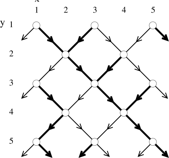
FIG. 1.: Lattice sites with bold lines indicating primary outlets. Forcing is applied in the direction of increasing $y$

FIG. 2.: Fraction of systems with a non-zero steady-steady current [$\Pi(p)$], steady-state current [$J(p)$] and fraction of sites in the drainage basin [$B(p)$] for a 1024x512 lattice averaged over 32 systems.

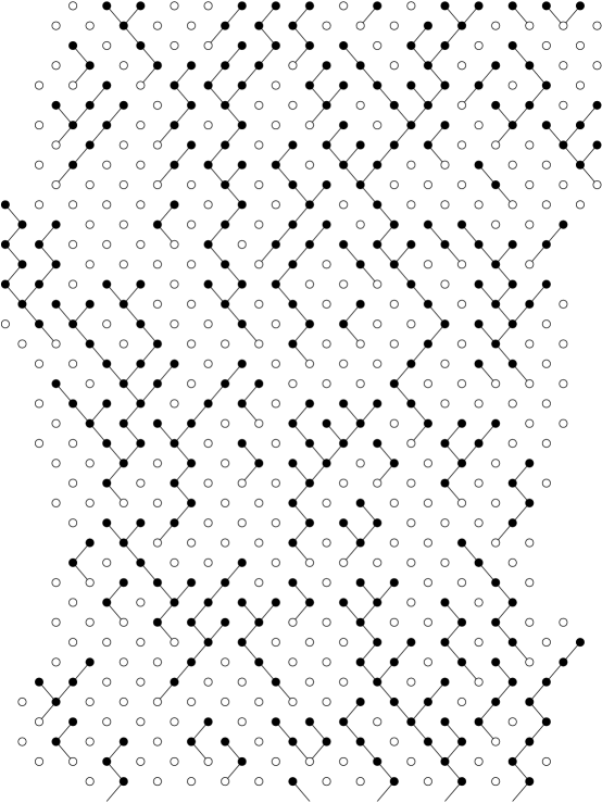
FIG. 3.: Lattice model below threshold. The black sites are saturated and the white sites are unsaturated. The lines show the primary outlets of each saturated site and form drainage trees. The force direction is down the page.

FIG. 4.: Fraction of systems that have a steady-state current for sudden and adiabatic increase of the force. Data use the same set of system sizes with widths $W=4L^{1/2}$ and using 512 samples for each.

FIG. 5.: Close up of $\Pi(p)$ curves for selected lengths with sudden forcing. Error bars are from measured sample variance. Crossing point is estimated as $p_{c}=0.3133\pm 0.0003$.

FIG. 6.: $\Pi$ finite size scaling with $p_{c}=0.3133$ and $\nu=1.62$ for systems of width $W=4L^{1/2}$

FIG. 7.: Width ($\Delta p$) of peak in $\partial\Pi/\partial p$ for systems of different lengths, and widths $W=4L^{1/2}$. Line has slope $-1/\nu$ with $\nu=1.62$.

FIG. 8.: Log-log plot of $J$ versus $(p-p_{c})$ for $p>p_{c}$ with $p_{c}=0.3133$. Line shown has slope $\beta=1.53$

FIG. 9.: Finite size scaling plot for $J$ using $p_{c}=0.3133$, $\nu=1.62$ and $\beta=1.53$.

FIG. 10.: Scaling of current at $p=0.3133$ with sample size, using $\beta/\nu=0.96$

FIG. 11.: Log-log plot for basin density.

FIG. 12.: Finite size scaling plot using $p_{c}=0.3133$, $\Gamma/\nu=0.29$ for the basin fraction $B$.

FIG. 13.: Scaling of drainage basin fraction at $p=0.3133$ with sample size using $\Gamma/\nu=0.302$

FIG. 14.: Tests for the width scaling for different values of $\alpha$. Simulations run at $\hat{p}_{c}(\alpha)$. Data for $\alpha=0.6$ is offset vertically by $+0.2$, data for $\alpha=0.5$ is offset by $+0.1$.

FIG. 15.: Log-log plot of current using the value $p=\hat{p}_{c}(\alpha)$ determined from using widths scaled with $\alpha=0.4$. Compare with Fig. 8

FIG. 16.: $\Pi$ finite size scaling for adiabatic increase with $p_{c,a}=0.299$ and $\nu_{a}=1.60$ and using narrow ($W=4L^{1/2}$) lattices

FIG. 17.: Channel network showing which outlets in the lattice carry current in the steady-state

FIG. 18.: Basic cumulative histogram data from one-deep model using $J=1/16$, $1/4$ and $1$ with system sizes $L=128$, $512$, $2048$. For a given $L$, the curves for larger $J$ are flatter.

FIG. 19.: Scaling of histograms for fixed occupancy fraction ($s$) with system size ($L$) and current ($J$)

FIG. 20.: Length scaled histogram data showing overlap for different values of $J$ for the large $L$ limit. Currents used are $J=1$, $J=1/2$, $J=1/4$, $J=1/8$ (only for $L>256$) and $J=1/16$ (only for $L>512$)

FIG. 21.: Data collapse for selected parameters: $J=1/8$ for $L=256,512,1024,2048$ and $J=1/16$ for $L=1024,2048$.

FIG. 22.: Histograms for current distribution from initial conditions with and without traps. Using a system of size 512x360. System with traps has p=0.35 and an average current of $J=0.0134$. Current without traps is chosen to be $J=0.0134$.

FIG. 23.: Test of the scaling form for $H(s)$ in the intermediate regime [Eq. (57)], using a range of system sizes from $L=128$ to $L=1024$ with $p$ and $J$ chosen so that $L^{2}\approx\xi_{f}\xi_{n}$ and with $0.02\leq s\leq 0.10$.

- [1] F. Nori, Science 271, 1373 (1996).
- [2] T. Matsuda et al., Science 271, 1393 (1996).
- [3] S. Bhattacharya and M. J. Higgins, Phys. Rev. B 49, 10005 (1994).
- [4] M. J. Higgins and S. Bhattacharya, Physica C 257, 232 (1996).
- [5] S. Bhattacharya and M. J. Higgins, Phys. Rev. Lett. 70, 2617 (1993).
- [6] A. C. Marley, M. J. Higgins, and S. Bhattacharya, Phys. Rev. Lett. 74, 3029 (1995).
- [7] U. Yaron et al., Nature 376, 753 (1995); 381, 253 (1996).
- [8] S. Bhattacharya and M. J. Higgins, Phys. Rev. B 52, 64 (1995).
- [9] M. C. Hellerqvist et al., Phys. Rev. Lett. 76, 4022 (1996).
- [10] N. Grønbech-Jensen, A. R. Bishop, and D. Domínguez, Phys. Rev. Lett. 76, 2985 (1996).
- [11] H. J. Jensen, A. Brass, and A. J. Berlinsky, Phys. Rev. Lett. 60, 1676 (1988).
- [12] H. J. Jensen, A. Brass, Y. Brecht, and A. J. Berlinsky, Phys. Rev. B 38, 9235 (1988).
- [13] A.-C. Shi and A. J. Berlinsky, Phys. Rev. Lett. 67, 1926 (1991).
- [14] M. C. Faleski, M. C. Marchetti, and A. A. Middleton, cond-mat/9605053 (unpublished).
- [15] K. Harada et al., Nature 360, 51 (1992).
- [16] K. Harada et al., Phys. Rev. Lett. 71, 3371 (1993).
- [17] K. Harada et al., Jpn. J. Appl. Phys. 33, 2534 (1994).
- [18] A. E. Koshelev and V. M. Vinokur, Phys. Rev. Lett. 73, 3580 (1994).
- [19] L. Balents and M. P. A. Fisher, Phys. Rev. Lett. 75, 4270 (1995).
- [20] O. Narayan and D. S. Fisher, Phys. Rev. B 49, 9469 (1994).
- [21] J. Watson and D. S. Fisher, Phys. Rev. B 54, 938 (1996).
- [22] O. Narayan and D. S. Fisher, Phys. Rev. B 46, 11520 (1992).
- [23] S. P. Obukhov, Physica A 101, 145 (1980).
- [24] D. Stuaffer and A. Aharony, Introduction to Percolation Theory, 2nd ed. (Taylor and Francis, London, 1991).
- [25] K. Binder and J.-S. Wang, J. Stat. Phys. 55, 87 (1989).
- [26] It is possible that the nonmonotonic convergence to scaling observed in the drainage basin may somehow be related to the presence of a second characteristic length scale above threshold, although why this should appear more strongly here than in is unclear.
- [27] A. P. Young, in Fundamental Problems in Statistical Mechanics VIII, Proceedings of the 1993 Altenberg Summer School, edited by H. van Beijeren and M. H. Ernst (North-Holland, Amsterdam, 1994).
- [28] W. Kinzel and J. M. Yeomans, J. Phys. A 14, L163 (1981).
- [29] A. B. Harris, J. Phys. C 7, 1671 (1974).
- [30] J. T. Chayes, L. Chayes, D. S. Fisher, and T. Spencer, Phys. Rev. Lett. 57, 2999 (1986).
- [31] Note that we did not need to use matching to the collision dominated network regime to derive the result ; in a collisionless system, the limit is pathological, but the physics discussed in the text is only consistent with the large limit of Eq. (55) if .
- [32] To obtain , it appears (at this point) that one has to consider the physics above threshold. This is somewhat analogous to certain conventional dynamic critical phenomena, such as superfluid 4He, in which a simple expression for the dynamic exponent can be obtained readily from physical arguments in one phase (the superfluid) but not in the other.[33]
- [33] P. C. Hohenberg and B. I. Halperin, Rev. Mod. Phys. 49, 435 (1977).