Spin-Gap Proximity Effect Mechanism of High Temperature Superconductivity

Abstract

When holes are doped into an antiferromagnetic insulator they form a slowly fluctuating array of “topological defects” (metallic stripes) in which the motion of the holes exhibits a self-organized quasi one-dimensional electronic character. The accompanying lateral confinement of the intervening Mott-insulating regions induces a spin gap or pseudogap in the environment of the stripes. We present a theory of underdoped high temperature superconductors and show that there is a local separation of spin and charge, and that the mobile holes on an individual stripe acquire a spin gap via pair hopping between the stripe and its environment; i.e. via a magnetic analog of the usual superconducting proximity effect. In this way a high pairing scale without a large mass renormalization is established despite the strong Coulomb repulsion between the holes. Thus the mechanism of pairing is the generation of a spin gap in spatially-confined Mott-insulating regions of the material in the proximity of the metallic stripes. At non-vanishing stripe densities, Josephson coupling between stripes produces a dimensional crossover to a state with long-range superconducting phase coherence. This picture is established by obtaining exact and well-controlled approximate solutions of a model of a one-dimensional electron gas in an active environment. An extended discussion of the experimental evidence supporting the relevance of these results to the cuprate superconductors is given.

]

I Introduction

Superconductivity in metals is the result of two distinct quantum phenomena, pairing and long-range phase coherence. In conventional homogeneous superconductors the phase stiffness is so great that these two phenomena occur simultaneously. On the other hand, in granular superconductors and Josephson junction arrays, pairing occurs at the bulk transition temperature of the constituent metal, while long-range phase coherence occurs, if at all, at a much lower temperature characteristic of the Josephson coupling between superconducting grains. High temperature superconductivity[1] is hard to achieve, even in theory, because it requires that both scales be elevated simultaneously–yet they are usually incompatible. Consider, for example, the strong-coupling limit of the negative $U$ Hubbard model [2] or the Holstein model [3]. Pairs have a large binding energy but, typically, they Bose condense at a very low temperature because of the large effective mass of a tightly bound pair. (The effective mass is proportional to $|U|$ in the Hubbard model and is exponentially large in the Holstein model.) A similar issue arises if the strong pairing occurs at specific locations in the lattice (negative-$U$ centers); in certain limits this problem may be mapped into a Kondo lattice[4], which displays heavy-fermion behavior.

A second problem for achieving high temperature superconductivity is that strong effective attractions, which might be expected to produce a high pairing scale, typically lead to lattice instabilities, charge or spin density wave order, or two-phase (gas-liquid or phase separated) states[5]. Here the problem is that the system either becomes an insulator or, if it remains metallic, the residual attraction is typically weak. In the neighborhood of such an ordered state there is a low-lying collective mode whose exchange is favorable for superconductivity, but the superconducting transition temperature is depressed by vertex corrections [6] and also because the density of states may be reduced by the development of a pseudogap.

A third (widely ignored) problem is how to achieve a high pairing scale at all in the presence of the repulsive Coulomb interaction, especially in a doped Mott insulator in which there is poor screening. A small coherence length (or pair size) implies that neither retardation, nor a long-range attractive interaction is effective in overcoming the bare Coulomb repulsion. Indeed, in the high temperature superconductors, angle resolved photoemission spectroscopy[7] (ARPES) suggests that the energy gap (and hence the pairing force) is a maximum for holes separated by one lattice spacing, where the bare Coulomb interaction is very large.

In short, superconductivity typically occurs at low temperatures: if any attractive interaction is weak the pairing energy is small; if it is strong the coherence scale is suppressed or the system is otherwise unstable. When this is coupled with the problem presented by the Coulomb force in a doped Mott insulator, the occurrence of high temperature superconductivity in the cuprate perovskites is even more remarkable. Indeed, there is evidence[8, 9, 10] that these materials live in a region of delicate balance between pairing and phase coherence: in “underdoped” and “optimally doped”materials, the onset of superconductivity is controlled by phase coherence, and occurs well below the pairing temperature, while in “overdoped” materials pairing and phase coherence take place at more or less the same temperature, as in more conventional superconductors. (See Fig. 1.) If we accept this point of view, then we can approach the problem of understanding the mechanism of high temperature superconductivity from the underdoped side by addressing three separate questions: i) What gives rise to the large temperature scale for pairing, or in other words for superconductivity on a local scale? ii) How can the system avoid the detrimental effects of strong pairing on global phase coherence? (i.e. large mass renormalizations.) iii) How can high temperature superconductivity with a short coherence length coexist with poor screening of the Coulomb interaction?

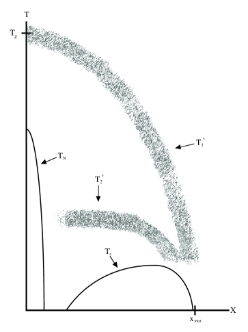
FIG. 1.: Theoretical sketch of the phase diagram for a high temperature superconductor in the doping-temperature plane. The solid lines represent phase transitions and the shaded areas crossovers. $T_{N}$ marks the transition to an antiferromagnetically ordered insulating state, and $T_{c}$ the transition to the superconducting state. $T_{1}^{*}$ marks the crossover temperature at which charge inhomogeneities (stripes) form and correspondingly local antiferromagnetic correlations develop in the insulating regions; the present paper is primarily concerned with the region between $T_{1}^{*}$ and somewhat above $T_{c}$, where the developing correlations are primarily confined to the neighborhood of an individual stripe. $T_{2}^{*}$ marks the temperature scale at which a spin gap develops in the 1DEG, and correspondingly the local superconducting susceptibility begins to diverge. Here, $T_{\chi}$, which is approximately $1/2$ the antiferromagnetic exchange energy, marks the temperature at which the antiferromagnetic correlation length in the undoped antiferromagnet is equal to two or three lattice constants. For further discussion, especially concerning the experimental justification for this figure, see Sec. IXC.

Here we shall argue that the high temperature superconductors resolve these problems in a unique manner: 1) The tendency of an antiferromagnet to expel holes[11] leads to the formation of hole-rich and hole-free regions[12]. For neutral holes this leads to a uniform instability (phase separation)[12] but, for charged holes, the competition with the long-range part of the Coulomb interaction generates a dynamical local charge inhomogeneity, in which the mobile holes are typically confined in “charged stripes”, separated by elongated regions of insulating antiferromagnet[13, 14, 15]. This self-organized collective structure, which we have named topological doping[16], is a general feature of doped Mott insulators, and it produces a locally quasi one-dimensional electronic character since, the electronic coupling between stripes falls exponentially with the distance between them [17]. 2) In a locally-striped structure, there is separation of spin and charge, as in the one-dimensional electron gas[18] (1DEG). Hence “pairing” is the formation of a spin gap, while the superfluid phase stiffness (i.e. the superfluid density divided by the effective mass) is a property of the collective charge modes[19, 20, 21]. 3) A large spin gap (or spin pseudogap) arises naturally in a spatially-confined, hole-free region, such as the medium between stripes. This effect is well documented for spin ladders[22], and for spin chains with sufficient frustration[23, 24]. The important point is that the spin gap does not conflict with the Coulomb interaction since the energetic cost of having localized holes in Cu $3d$ orbitals has been paid in the formation of the material. 4) The spin degrees of freedom of the 1DEG acquire a spin gap by pair hopping between the stripe and the antiferromagnetic environment. (Single particle tunnelling is irrelevant[25].) At the same time, because of the local separation of spin and charge, the spin-gap fixed point is stable even in the presence of strong Coulomb interactions, and there is no mass renormalization to depress the onset of phase coherence, so the superconducting susceptibility diverges strongly below this temperature[26].

In summary, the “mechanism” of high temperature superconductivity is a form of magnetic proximity effect in which a spin gap is generated in Mott-insulating antiferromagnetic regions through spatial confinement by charge stripes, and communicated to the stripes by pair hopping. The mobile holes on the stripes have the large phase stiffness required for a high superconducting transition temperature.

The formation of a spin gap in the 1DEG may be regarded as a pairing of “spinons”, i.e. the neutral, spin-1/2 soliton excitations which occur in the low energy spectrum of the 1DEG and a number of one-dimensional quantum antiferromagnets. Indeed, local inhomogeneity provides a realization of some of the earlier ideas[27] involving spin-charge separation in the high temperature superconductors and the concept of a spin liquid, by which we mean a quantum disordered system (i.e. with unbroken spin-rotation symmetry) which supports spinons in its physical spectrum. However, we emphasise that previous ideas relied on a putative two-dimensional spin-liquid fixed point, while here we are dealing with a locally one-dimensional system, for which it is well established[18, 20] that separation of spin and charge [18] occurs generically, and there exists a “paired spin-liquid” phase, i.e. a spin-liquid with a finite gap or pseudogap in the spinon spectrum. (See discussion in Appendix C.) In the strictest sense then, both are intermediate-distance effects[37] which occur below a dimensional-crossover scale to two (or three) dimensional physics.

We thus view the emergence of high temperature superconductivity as a three-stage process, which can be described in renormalization group language in terms of the influence of three fixed points. At high temperatures, the “avoided critical phenomena”[15] associated with frustrated phase separation, govern the emergence of the self-organized, quasi one-dimensional structures. At intermediate temperatures, the one-dimensional paired spin liquid fixed point controls the pairing scale, and the growth of local superconducting (and CDW) correlations. Finally, at low temperatures, a two (or three) dimensional fixed point determines the long-distance physics and the ultimate superconducting or insulating behavior of the system.

Our proposed mechanism implies the existence of two crossover scales above $T_{c}$ in underdoped materials, as shown in Fig. 1: a high temperature scale, at which local stripe order and antiferromagnetic correlations develop, and a lower temperature at which local pairing (spin gap) and significant superconducting correlations appear on individual charge stripes. $T_{c}$ itself, is then determined by the Josephson coupling between stripes, i.e. by the onset of global phase coherence [8].

The local charge inhomogeneity which is a central feature of our model has substantial support from experiment. In the past few years charge ordering has been discovered in a number of layered oxides, such as La_2-xSr_xNiO_4+δ[38] and La_0.5Sr_1.5MnO₄[39], and there is considerable experimental evidence showing that the high temperature superconductors display a coexistence of superconductivity and charge inhomogeneity. In particular, the efficient destruction of the antiferromagnetic order [40] of the parent insulating state is a consequence of topological doping [16], in which the mobile holes form metallic stripes that are antiphase domain walls for the spins. The stripes may be ordered[41] (as in La_1.6-xNd_0.4Sr_xCuO₄), dynamically fluctuating [41, 42] (as in optimally-doped La_2-xSr_xCuO₄), or pinned and meandering [43] (as in lightly doped La_2-xSr_xCuO₄). Thus, we consider the existence of local metallic stripes (at least in the La₂CuO₄ family of high temperature superconductors) to be an experimental fact. Evidence of specific charge fluctuations in any family of cuprate superconductors suggests that they are an important ingredient in the theory of high temperature superconductivity. However neutron scattering data[44] also suggest that there are similar, but more disordered, structures[15] in underdoped YBa₂Cu₃O_7-δ. An analysis of ARPES experiments on Bi₂Sr₂CaCu₂O_8+δ leads to a similar conclusion[45].

The systematics of phase fluctuations [8], mentioned above, strongly suggests that pairing on a high energy scale does not require interaction between metallic charge stripes, although T_c is certainly controlled by the Josephson coupling required to establish phase coherence for an array of stripes. Consequently, it should be possible to understand the mechanism of pairing from the behavior of a single stripe, modelled as a 1DEG coupled to the various low-lying states of an insulating environment. A complete discussion of this problem is a substantial generalization of the theory of the one-dimensional electron gas [46] which will be considered more completely in a subsequent publication [47]. Here it will be shown that, for the high temperature superconductors, the most important process is the hopping of a pair of holes from the stripe into the antiferromagnetic environment, which also may be regarded as a coherent form of transverse stripe fluctuation. It will be shown that the stripe develops a spin gap which, in this model, corresponds to pairing without phase coherence. We consider two situations: a) the antiferromagnetic environment has a pre-existing spin gap or spin pseudogap because of its finite spatial dimensions[22] and b) pair hopping produces a spin gap in both the stripe and the environment. In the first case, we find that an induced spin gap in the 1DEG and the consequent divergent superconducting fluctuations are a robust consequence of the coupling to the environment. The second case requires a sufficiently strong (and possibly unphysical) Coulomb interaction between holes on the stripe and holes in the environment for pair tunnelling to be relevant.

Although the existence of two distinct regions, the stripe and the antiferromagnetic environment, provides a potential escape from some of the limitations on the superconducting transition temperature T_c, it is not a priori obvious that a large mass renormalization can be avoided. Indeed, the model we shall study is closely related to Kondo lattice models[4], for which heavy-fermion behavior or large mass renormalization is the primary consequence of the strong interactions. However we find that, for stripes in an antiferromagnet (as for one-dimensional Kondo and orbital Kondo lattice models [48, 49]), the analog of heavy-fermion physics is reflected solely in the the spin degrees of freedom while for the charge modes, and hence the superfluid phase stiffness, the mass is not renormalized!

In some respects, what we are doing is analogous to working out the renormalization of the electron self energy by the coupling to phonons. However, the calculation is more complicated because, here, the elementary objects are strings of charge (stripes) in a polarizable medium that profoundly influences their internal structure. Fluctuating stripes are of finite length but the solution of the infinite 1DEG may be used if they are longer than the spin gap length scale, which is a few lattice spacings[22].

Of course, at higher hole concentrations, the calculation must be modified to take account of the interaction between the stripes, especially to obtain long-range superconducting order. In general terms, it is fairly straightforward to see how global superconductivity arises in a system with a small but finite density of ordered or slowly-fluctuating stripes, as found in underdoped members of the La_2-xSr_xCuO₄ family of superconductors. Indeed, an analysis of neutron scattering and thermodynamic data for underdoped and optimally doped La_2-xSr_xCuO₄[42] suggests that T_c is proportional to the product of the Drude weight of the holes on a stripe and the stripe concentration c_s.

An interesting feature of our model is the interplay between the short-distance physics associated with the fluctuating stripes and the ultimate long-range order that is established in a given material. We shall show that both superconducting and charge density wave correlations develop on a given stripe. However, they compete at longer length scales, although they may coexist in certain regions of the phase diagram. Also it follows from general principles that, locally, the singlet superconducting order parameter will be a strong admixture of extended-$s$ and d${}_{x^{2}-y^{2}}$ states. Ultimately, in tetragonal materials, the order parameter must have a pure symmetry, but the way in which it emerges from the short-distance physics is very different from more conventional routes.

This paper is quite long and, in parts, rather technical. It addresses the purely theoretical problem of constructing and solving a general model of a 1DEG in an active environment. At the same time, we wish to report progress on the key problem of understanding the mechansim of high temperature superconductivity in the cuprate superconductors. To compensate, we have attempted to make the various sections as self-contained as possible, and to indicate which sections can be skipped by the reader with a more focussed interest in the problem.

A rather general model of the interactiong 1DEG in an active environment is introduced in Sec. II. The model is bosonized in Sec. III, and various formal transformations that are useful for later analysis are described; this section also contains a discussion of which of the allowed interactions in the model are unimportant for our purposes, and so can be ignored. In Sec. IV, we define a simplified “pseudospin” model of the charge excitations of the environment, and argue that it exhibits the same low-energy physics as the general model. Sec. V contains a discussion of exact results for the zero temperature properties of the pseudospin model, which among other things exhibits the spin-gap proximity effect, and the generation of a paired spin liquid state of the 1DEG, even in the presence of arbitrarily-strong forward scattering. Section VI reports the results of a controlled approximate solution of the pseudospin model for a wide range of temperatures and coupling constants; in particular, various crossover temperatures to spin-gap behavior are identified, and their dependence on the interactions in the model are determined. In Sec. VII, we return to the problem of the charge degrees of freedom of the 1DEG, and consider the effects of umklapp scattering in conditions of near commensurability, and the effects of an externally applied potential. In Sec. VIII, we digress slightly to consider the effects of a “spin-gap center” on the local properties of a Fermi liquid. Finally, in Sec. IX, we summarize our results and discuss experimental implications and predictions for the high temperature superconductors. In this section, we also suggest some numerical calculations to test the major ideas. The reader who is primarily interested in a discussion of results may skip directly to Sec. IX. In addition, Appendix A recasts some of the present discussion in the familiar language of the perturbative renormalization group for the 1DEG, Appendix B contains an analysis of the symmetries of the model, and an explicit construction of the non-local order parameter which characterizes “local pairing”, and Appendix C discusses the precise nature of the paired-spin-liquid state, and gives concrete examples of model systems which exhibit this state.

II The 1DEG in an Active Environment

A The problem and the solution strategy

It has long been realized that the low energy properties of a one dimensional electron gas (1DEG), and indeed of a wide variety of other interacting one dimensional systems, are equivalent to those of the simplest field theory of interacting electrons, characterized by a small number of potentially relevant interactions between electrons at the Fermi surface. In this section we address the problem of a 1DEG in an “active” environment, one that possesses its own low-energy excitations which couple to the 1DEG, but is insulating so that the electrons of the 1DEG may make excursions into the environment, but ultimately return. The environment in which we are interested is antiferromagnetic, so it may have low-energy spin excitations. It will also have low-energy charge excitations in which holes make excursions from the metallic stripe into the environment. Their energy is low because frustrated phase separation, which generates metallic stripes in the first place, involves a delicate balance of Coulomb and magnetic energies.

This problem can be addressed in several distinct ways. In the present paper, we make extensive use of a renormalization group strategy involving exact solutions of solvable models, together with a sophisticated approximate calculation, in which the fluctuations of the 1DEG and the environment are solved exactly, but the coupling between them is treated in a mean-field approximation. We also give physical estimates of the values of the various coupling constants that enter the model, and present strong physical arguments to show that the physical systems of interest will lie in the “basin of attraction” of the strong-coupling fixed point that governs the behavior of the solvable models. In Section IX, we will also outline some simple one-dimensional lattice models which are amenable to numerical solution, and are expected to exhibit the mechanism described in this paper.

B The general model

To begin with, we consider a very general model of a 1DEG coupled to an environment. The initial form of the model is microscopically realistic. It will be assumed that the environment itself is a one dimensional system with a charge gap (since it is an insulating matrix) which may or may not have a spin gap. We thus consider the Hamiltonian to be of the form

$$H=\int_{-\infty}^{\infty}dx\big{[}{\cal H}_{1DEG}+{\cal H}_{env}+{\cal H}_{int}+{\cal H}_{coul}\big{]}.$$ (1)

The bare Hamiltonian density of the 1DEG is

$${\cal H}_{1DEG}={\cal H}_{0}+{\cal H}_{1}.$$ (2)

Here ${\cal H}_{0}$ is the Hamiltonian of a non-interacting 1DEG, which in the continuum limit can be written (with $\hbar=1$) as

$${\cal H}_{0}= iv_{F}\sum_{\sigma}\left[\psi^{\dagger}_{1,\sigma}\partial_{x}\psi_{1,\sigma}-\psi^{\dagger}_{2,\sigma}\partial_{x}\psi_{2,\sigma}\right]$$ (4)

$$-\mu\sum_{\alpha,\sigma}\left[\psi^{\dagger}_{\alpha,\sigma}(x)\psi_{\alpha,\sigma}(x)\right]$$

where $\psi^{\dagger}_{\alpha,\sigma}(x)$ creates an electron with z component of spin $\sigma$ on the right or left moving branch of the Fermi surface for $\alpha=1$ or $2$ respectively. Here, we have made a Galilean transformations to shift the Fermi points to $k=0$; factors involving the Fermi wave vector $k_{F}$ will be shown explicitly. ${\cal H}_{1}$ incorporates the electron-electron interactions within the 1DEG and has the continuum form [46]

$${\cal H}_{1}= g_{2}\sum_{\sigma,\sigma^{\prime}}\psi^{\dagger}_{1,\sigma}\psi^{\dagger}_{2,\sigma^{\prime}}\psi_{2,\sigma^{\prime}}\psi_{1,\sigma}$$ (7)

$$+g_{1}\sum_{\sigma,\sigma^{\prime}}\psi^{\dagger}_{1,\sigma}\psi^{\dagger}_{2,\sigma^{\prime}}\psi_{1,\sigma^{\prime}}\psi_{2,\sigma}$$

$$+g_{3}\big{[}\psi_{1,\uparrow}^{\dagger}\psi_{1,\downarrow}^{\dagger}\psi_{2,\downarrow}\psi_{2,\uparrow}e^{i(4k_{F}-G)x}+H.c.\big{]}.$$

Here $G$ is a reciprocal lattice vector and $g_{3}$ is the coupling constant for umklapp scattering. When the 1DEG is incommensurate $(4k_{F}\neq G)$, the rapid phase oscillations in the term proportional to $g_{3}$ render it irrelevant in the renormalization group sense. However, near to commensurability, this term is responsible for the fact that the Drude weight is proportional to the density of doped holes, as we shall see. Typically, it will be assumed that the interactions are repulsive ($g_{1},g_{2},g_{3}>0$) although they may undergo significant renormalization by the coupling of the 1DEG to the high energy excitations of the antiferromagnetic environment (which we do not consider explicitly). The parameters that describe the 1DEG are thus the Fermi velocity, $v_{F}$, the chemical potential, $\mu$, the three coupling constants $g_{i}$, and the “incommensurability”, $4k_{F}-G$. It should be emphasised that this is a very general representation of the low-energy physics of a stripe in a CuO₂ plane, and all details of the original microscopic model are contained in the values of the coupling constants $g_{i}$.

We have in mind the low-density limit of a stripe phase in which the Coulomb interaction on a given stripe is screened by the motion of charge on neighboring stripes, and so does not make a singular contribution to the forward scattering interaction, $g_{2}$. Thus, for the time being, we will neglect the term ${\cal H}_{coul}$, although it will ultimately play a role in the dynamics of the superconducting phase [9].

Because the physics of interacting systems in one dimension is ultimately so constrained, it is possible to model the Hamiltonian density of the environment as a second (distinct) interacting one dimensional electron gas. The Hamiltonian ${\cal H}_{env}$ has the same form as in Eqs. (4) and (7), except that fields and parameters will be marked with a super-tilde. However there are several important differences in the parameters of the Hamiltonian: 1) The environment is a Mott insulator. Consequently there is a strong commensurability energy ($4{\tilde{k}}_{F}=\tilde{G}$ and ${\tilde{g}}_{3}$ is large), which produces a gap in the the charge degrees of freedom of the environment. This also implies that ${\tilde{k}}_{F}$ is different from $k_{F}$. 2) Because of the frustration of the motion of holes in an antiferromagnet, [50] the propagation velocity $\tilde{v}_{c}$ for charge excitations in the environment is much smaller than the corresponding velocity in the 1DEG. This is the primary manner in which the driving force for phase separation [12] and stripe formation [14, 15] appears in the model. 3) We shall consider three possibilities for the spin degrees of freedom of the environment, one in which there are gapless magnon-like excitations, and two in which there is a spin gap: a) The gapless state is realized by considering the model with $\tilde{g}_{1}>0$, in which case the environmental spin excitations are those of an antiferromagnetic spin-1/2 Heisenberg chain. b) A spin gap can occur with an accompanying spontaneous breaking of translational (chiral) symmetry (See Appendix B), which is realized by simply taking $\tilde{g}_{1}<0$, in which case the environmental spin excitations are those of a spin-1/2 Heisenberg chain with competing nearest and next-nearest neighbor antiferromagnetic interactions, e.g. the Majumdar-Ghosh model.[24] c) A spin-gap can occur without any accompanying broken symmetry, in the manner of the antiferromagnetic two leg, spin 1/2 Heisenberg ladder[22]; to model this system, we need to add a backscattering term to the environmental Hamiltonian (of the same form as $H_{e}$ in Eq. (125), below), although a better description can be attained in the bosonized form of the Hamiltonian, as discussed below. For our purposes, there is no significant difference in the implications of the two types of environmental spin gap, so for simplicity, we will perform our calculations for the case in which the spin gap is induced by a negative $\tilde{g}_{1}$, and will use language to describe the physics that (properly) does not distinguish the two types of environmental spin gap.

Using well known results for the 1DEG, it is possible to express these coupling constants in terms of the physical variables which define the excitation spectrum of the environment: the spin and charge velocities, ${\tilde{v}}_{s}$ and ${\tilde{v}}_{c}$, the charge gap ${\tilde{\Delta}}_{c}$ and the spin gap (if one exists) ${\tilde{\Delta}}_{s}$, and the charge and spin correlation exponents (defined below), $\tilde{K}_{c}$ and $\tilde{K}_{s}$. Since the environment is an insulator, we will always assume that ${\tilde{\Delta}}_{c}$ is large. We also must include the energy $\epsilon$ to transfer charge from the 1DEG to the environment. For the case of “p-type” doping, in which $\tilde{\mu}$ lies in the lower half of the environmental gap, $\varepsilon/2\equiv{\tilde{\Delta}}_{c}-[\tilde{\mu}-\mu]$ is the bare energy required to remove a quantum of charge from the environment and add it to the 1DEG. We will be interested in the case $0\leq\varepsilon\ll{\tilde{\Delta}}_{c}$.

Finally, we consider the coupling between the 1DEG and the environment, for which spin-rotational invariance and conservation of momentum along the stripe direction severely limit the number of possible relevant interactions. Since the Fermi wave vector of the 1DEG is incommensurate with the wave vector of any low energy excitation of the environment, we can neglect, as irrelevant, terms which transfer momentum $\pm k_{F}$ or $\pm 2k_{F}$ between the 1DEG and the environment. For example there are no low energy single-particle hopping processes, even though, at the microscopic level, one might expect them to have the largest coupling term. Such processes are included implicitly as virtual intermediate states in constructing the effective low energy Hamiltonian. (We will return to this point briefly in the following section.) With this in mind, the most general form of the interaction Hamiltonian density, i.e. which keeps all potentially relevant terms, is

$${\cal H}_{int}= J_{s}{\vec{j}}_{s}\cdot{\vec{\tilde{j}}}_{s}+V_{s}{\vec{S}}\cdot{\vec{\tilde{S}}}$$ (10)

$$+J_{c}j_{c}{\tilde{j}}_{c}+V_{c}\rho{\tilde{\rho}}$$

$$+{\cal H}_{pair},$$

where the small momentum transfer couplings involve the long-wavelength density fluctuations relative to the background charge density $\rho_{0}$

$$\rho(x)-\rho_{0}=\sum_{\sigma}\big{[}\psi_{1,\sigma}^{\dagger}\psi_{1,\sigma}+\psi_{2,\sigma}^{\dagger}\psi_{2,\sigma}\big{]},$$ (11)

the bare charge-current operator

$$j_{c}(x)=\sum_{\sigma}\big{[}\psi_{1,\sigma}^{\dagger}\psi_{1,\sigma}-\psi_{2,\sigma}^{\dagger}\psi_{2,\sigma}\big{]},$$ (12)

the long-wavelength spin density operator

$${\vec{S}}(x)=\sum_{\sigma,\sigma^{\prime}}\big{[}\psi_{1,\sigma}^{\dagger}{\vec{\sigma}}_{\sigma,\sigma^{\prime}}\psi_{1,\sigma^{\prime}}+\psi_{2,\sigma}^{\dagger}{\vec{\sigma}}_{\sigma,\sigma^{\prime}}\psi_{2,\sigma^{\prime}}\big{]},$$ (13)

and the bare spin-current operator

$${\vec{j}}_{s}(x)=\sum_{\sigma,\sigma^{\prime}}\big{[}\psi_{1,\sigma}^{\dagger}{\vec{\sigma}}_{\sigma,\sigma^{\prime}}\psi_{1,\sigma^{\prime}}-\psi_{2,\sigma}^{\dagger}{\vec{\sigma}}_{\sigma,\sigma^{\prime}}\psi_{2,\sigma^{\prime}}\big{]}.$$ (14)

The corresponding operators for the environment are defined by the same equations, except that all quantities have a super-tilde. Note that we have chosen to express ${\cal H}_{int}$ in terms of the charge and spin current operators for the noninteracting system. The other contribution to ${\cal H}_{int}$ is the pair transfer terms

$${\cal H}_{pair}= t_{sp}\big{[}P^{\dagger}{\tilde{P}}+{\rm H.c.}\big{]}$$ (15)

$$+ t_{tp}\sum_{m=-1}^{1}\big{[}{P}_{m}^{\dagger}{{\tilde{P}}}_{m}+{\rm H.c.}\big{]}$$ (16)

where for the 1DEG, $P^{\dagger}$ is the usual singlet pair creation operator,

$$P^{\dagger}(x)\equiv\frac{1}{\sqrt{2}}\left[\psi^{\dagger}_{1,\uparrow}(x)\psi^{\dagger}_{2,\downarrow}(x)+\psi^{\dagger}_{2,\uparrow}(x)\psi^{\dagger}_{1,\downarrow}(x)\right],$$ (17)

and $P_{m}$ are the componenets of the triplet pair creation operator,

$$P^{\dagger}_{1}(x) \equiv \psi_{1,\uparrow}^{\dagger}\psi_{2,\uparrow}^{\dagger}$$ (18)

$$P_{0}^{\dagger}(x) \equiv \frac{1}{\sqrt{2}}\left[\psi^{\dagger}_{1,\uparrow}(x)\psi^{\dagger}_{2,\downarrow}(x)-\psi^{\dagger}_{2,\uparrow}(x)\psi^{\dagger}_{1,\downarrow}(x)\right]$$ (19)

$$P^{\dagger}_{-1} \equiv \psi_{1,\downarrow}^{\dagger}\psi_{2,\downarrow}^{\dagger}.$$ (20)

III Bosonization of the Model

In dealing with the problem of the 1DEG in an active environment, it is useful to rewrite the model using the standard boson representation of Fermi fields in one dimension [46]:

$$\psi^{\dagger}_{\lambda,\sigma}(x)=\frac{1}{\sqrt{2\pi a}}exp\{i\Phi_{\lambda,\sigma}(x)\}$$ (21)

where $\Phi_{\lambda,\sigma}=\sqrt{\pi}[\theta_{\sigma}(x)\pm\phi_{\sigma}(x)]$ with “-” and “+” corresponding to $\lambda=1$ and $2$ respectively, $\theta_{\sigma}(x)=\int_{-\infty}^{x}dx^{\prime}\Pi_{\sigma}(x^{\prime})$, and $\phi_{\sigma}(x)$ and $\Pi_{\sigma}(x)$ are canonically conjugate Bose fields, so that $[\phi_{\sigma}(x),\Pi_{\sigma^{\prime}}(x^{\prime})]=i\delta(x-x^{\prime})$. ($\theta$ and $\phi$ are thus dual to each other in the usual statistical mechanical sense of order and disorder variables.) To take advantage of the separation of spin and charge [46], the Hamiltonian will be expressed in terms of a spin field, $\phi_{s}(x)=[\phi_{\uparrow}-\phi_{\downarrow}]/\sqrt{2}$, and a charge field, $\phi_{c}(x)=[\phi_{\uparrow}+\phi_{\downarrow}]/\sqrt{2}$ and their conjugate momenta: $\Pi_{s}(x)=[\Pi_{\uparrow}-\Pi_{\downarrow}]/\sqrt{2}$ and $\Pi_{c}(x)=[\Pi_{\uparrow}+\Pi_{\downarrow}]/\sqrt{2}$. The charge and spin density and current operators may be written:

$$\rho(x) = -\sqrt{2\over\pi}\ \partial_{x}\phi_{c}$$ (22)

$$j_{c}(x) = \sqrt{2\over\pi}\ \Pi_{c}$$ (23)

$$S^{z}(x) = -\sqrt{1\over 2\pi}\ \partial_{x}\phi_{s}$$ (24)

$$S^{\pm}(x) = {1\over\pi a}\exp(\pm i\sqrt{2\pi}\theta_{s})\cos[\sqrt{2\pi}\phi_{s}]$$ (25)

$$j_{s}^{z}(x) = \sqrt{1\over 2\pi}\ \Pi_{s}$$ (26)

$$j_{s}^{\pm}(x) = {-i\over\pi a}\exp(\pm i\sqrt{2\pi}\theta_{s})\sin[\sqrt{2\pi}\phi_{s}].$$ (27)

In terms of these variables, the Hamiltonians of the stripe, the environment, and the small-momentum transfer coupling between the two may be written as a sum of a charge-only part and a spin-only part. However, the pair hopping terms $H_{pair}$ introduces a coupling between spin and charge. Thus the total Hamiltonian may be written

$${\cal H}={\cal H}_{c}+{\cal H}_{s}+{\cal H}_{pair}.$$ (28)

We now consider the various contributions in turn.

A Spin Degrees of Freedom

The general form of the spin Hamiltonian is

$${\cal H}_{s}\equiv{\cal H}_{s}^{0}+{\cal H}_{s}^{1}+{\cal H}_{s}^{2}$$ (29)

Here

$${\cal H}_{s}^{0} = \frac{v_{s}}{2}[K_{s}\Pi_{s}^{2}+\frac{1}{K_{s}}(\partial_{x}\phi_{s})^{2}]$$ (30)

$$+ \frac{\tilde{v}_{s}}{2}[\tilde{K}_{s}\tilde{\Pi}_{s}^{2}+\frac{1}{\tilde{K}_{s}}(\partial_{x}\tilde{\phi}_{s})^{2}],$$ (31)

$${\cal H}_{s}^{1}=\frac{2J_{s}}{\pi}\Pi_{s}(x)\tilde{\Pi}_{s}(x)+\frac{2V_{s}}{\pi}\partial_{x}\phi_{s}(x)\tilde{\partial}_{x}\phi_{s}(x),$$ (32)

and

$${\cal H}_{s}^{2}= \frac{2g_{1}}{(2\pi a)^{2}}\cos\big{[}\sqrt{8\pi}\phi_{s}\big{]}$$ (33)

$$+ \frac{2\tilde{g}_{1}}{(2\pi a)^{2}}\cos\big{[}\sqrt{8\pi}\tilde{\phi}_{s}\big{]}$$ . (34)

$$+ \frac{V_{s}}{2\pi a}\cos\big{[}\sqrt{2\pi}(\theta_{s}-\tilde{\theta}_{s})\big{]}\cos\big{[}\sqrt{2\pi}\phi_{s}\big{]}\cos\big{[}\sqrt{2\pi}\tilde{\phi}_{s}\big{]}$$ (35)

$$+ \frac{J_{s}}{2\pi a}\cos\big{[}\sqrt{2\pi}(\theta_{s}-\tilde{\theta}_{s})\big{]}\sin\big{[}\sqrt{2\pi}\phi_{s}\big{]}\sin\big{[}\sqrt{2\pi}\tilde{\phi}_{s}\big{]}$$ (36)

Here $v_{s}$ is the spin-wave velocity and $K_{s}$ is the critical exponent[51] that specifies the location on a line of fixed points. Also $v_{s}$ is given by $v_{s}=2v_{F}K_{s}/(K_{s}^{2}+1)$. In the absence of coupling between the stripe and the environment, the Hamiltonian is known to be correct for weak or strong coupling and for different forms of short-distance or high-energy cutoff [46], although it may be necessary to perform some form of global renormalization to determine $K_{s}$ from the parameters of the initial Hamiltonian. For weak coupling, $K_{s}$ is related to the bare Fermi velocity $v_{F}$ and coupling constants as $K_{s}=\sqrt{\frac{2\pi v_{F}+g_{1}}{2\pi v_{F}-g_{1}}}$. For repulsive interactions (i.e. $g_{1}>0$) one finds $K_{s}>1$.

For the case in which $\tilde{g}_{1}$ is negative and relevant, in the renormalization group sense, there is a two fold degenerate ground state, corresponding to the classical values $\tilde{\phi}_{s}=0$ and $\tilde{\phi}_{s}=\sqrt{\pi/2}$. (See Appendix B.) To represent the case in which there is an environmental spin gap without symmetry breaking, we should add a term proportional to $\cos[\sqrt{2\pi}\tilde{\phi}_{s}]$, which arises in a microscopic system with two spins per unit cell, such as a two-leg ladder[52]. This term (which may be generalized to allow any even number of spins per unit cell) is always relevant for repulsive interactions, so it always leads to a spin gap. As we shall see shortly, the important point is that a spin gap of whatever origin implies a quenching of the fluctuations of $\tilde{\phi}_{s}$. For a caveat on commensurability effects, see Sec. VII.

B Charge Degrees of Freedom

The general form of the charge Hamiltonian is

$${\cal H}_{c}={\cal H}_{c}^{0}+{\cal H}_{c}^{1}+{\cal H}_{c}^{2},$$ (37)

where

$${\cal H}_{c}^{0} = \frac{v_{c}}{2}[K_{c}\Pi_{c}^{2}+\frac{1}{K_{c}}(\partial_{x}\phi_{c})^{2}]$$ (38)

$$+ \frac{\tilde{v}_{c}}{2}[\tilde{K}_{c}\tilde{\Pi}_{c}^{2}+\frac{1}{\tilde{K}_{c}}(\partial_{x}\tilde{\phi}_{c})^{2}],$$ (39)

$${\cal H}_{c}^{1} = \frac{2J_{c}}{\pi}\Pi_{c}\tilde{\Pi}_{c}+\frac{2V_{c}}{\pi}\partial_{x}\phi_{c}\partial_{x}\tilde{\phi}_{c},$$ (40)

and

$${\cal H}_{c}^{2}= \frac{2g_{3}}{(2\pi a)^{2}}\cos\big{[}\sqrt{8\pi}\ \phi_{c}-(4k_{F}-G)x\big{]}$$ (41)

$$+ \frac{2\tilde{g}_{3}}{(2\pi a)^{2}}\cos\big{[}\sqrt{8\pi}\tilde{\phi}_{c}\big{]}-\tilde{\mu}\sqrt{{2\over\pi}}\ \partial_{x}\tilde{\phi}_{c}.$$ (42)

Here $v_{c}$ is the charge velocity and $K_{c}$ is the Luttinger liquid exponent [51], with $v_{c}=2v_{F}K_{c}/(K_{c}^{2}+1)$. For weak coupling, $K_{c}$ is related to the bare Fermi velocity $v_{F}$ and coupling constants as $K_{c}=\sqrt{\frac{2\pi v_{F}+g_{c}}{2\pi v_{F}-g_{c}}}$ , where $g_{c}=g_{1}-2g_{2}$. For repulsive interactions $0<K_{c}<1$ (i.e. $g_{c}<0$).

C Spin-Charge Coupling

Pair hopping between the stripe and the environment, as given by ${\cal H}_{pair}$, destroys the separation of spin and charge and is the driving force for much of the interesting physics. Its bosonized form is given by

$${\cal H}_{pair}= \bigg{(}{t_{sp}\over\pi^{2}a^{2}}\bigg{)}\cos[\sqrt{2\pi}(\theta_{c}-{\tilde{\theta}_{c}})]\cos[\sqrt{2\pi}\phi_{s}]\cos[\sqrt{2\pi}{\tilde{\phi}_{s}}]$$ (43)

$$+ \bigg{(}{t_{tp}\over\pi^{2}a^{2}}\bigg{)}\bigg{\{}\cos[\sqrt{2\pi}(\theta_{c}-{\tilde{\theta}_{c}})]\cos[\sqrt{2\pi}(\theta_{s}-{\tilde{\theta}_{s}})]$$ (45)

$$-\cos[\sqrt{2\pi}(\theta_{c}-{\tilde{\theta}_{c}})]\sin[\sqrt{2\pi}\phi_{s}]\sin[\sqrt{2\pi}{\tilde{\phi}_{s}}]\bigg{\}}.$$

D Which Terms Are Unimportant?

The general model has numerous coupling constants, and so, for much of this paper, we focus on the terms that are most important for our purposes, and set the others to zero. Specifically, we drop those terms which are, in the renormalization group sense, irrelevant at the paired spin liquid fixed point. This argument simply shows that dropping these terms is self consistent. However, given the nature of the antiferromagnetic environment, there are strong arguments to show that these terms also are physically irrelevant, i.e. that the physical system lies in the basin of attraction of the paired spin liquid fixed point.

To begin with, we examine the magnetic interactions, $J_{s}$ and $V_{s}$ in ${\cal H}_{int}$: these terms represent the interaction between the ferromagnetic fluctuations in the two sub-systems. Since we are primarily interested in antiferromagnetic systems, we do not expect these terms ever to be important. Of course, in the paired spin liquid state, or more generally in the presence of any sort of environmental spin gap, this can be seen directly from their dependence on $\tilde{\theta}_{s}$, which means that the corresponding correlation functions decay exponentially with distance or time, and are thus trivially irrelevant. The triplet pair-tunnelling term similarly depends on $\tilde{\theta}_{s}$, and correspondingly triplet pairing is generally expected to be important only in nearly ferromagnetic systems. Therefore, on both clear physical, and formal renormalization group grounds, it is safe to simplify our further discussion by taking

$$J_{s}=V_{s}=t_{tp}=0,$$ (46)

unless explicitly stated otherwise.

Thus, in the case where there is strong incommensurability between the values of $k_{F}$ in the two subsystems, and neither has significant ferromagnetic fluctuations, the only important interactions between the 1DEG and the environment are $t_{sp}$, $V_{c}$, and $J_{c}$.

Away from half filling, the renormalization of the umklapp scattering coupling constant $g_{3}$ is cut off by the incommensurability[53, 20], and for some purposes it may be dropped. However, this does not mean that umklapp scattering is unimportant for the low energy physics. Doping of holes into the Mott insulating state in one dimension creates soliton excitations[53, 54] in the charge density with a mass governed by $g_{3}$. There is a “doped-insulator” region in which these excitations control the Drude weight and the superfluid phase stiffness. In our stripe model of the cuprates, high temperature superconductivity may occur within this region of doping.

Finally, we address the non-linear term proportional to $g_{1}$ in ${\cal H}_{s}^{2}$ in Eq. (33). For repulsive interactions, i.e. for $K_{s}>1$, this term is perturbatively irrelevant, and the renormalization group flows go to the fixed point $g_{1}=0$ and $K_{s}=1$. (See Appendix A.) Thus, so long as the bare interactions in the 1DEG are not too large, it is reasonable to use the fixed point values

$$g_{1}=0\ \ {\rm and}\ \ K_{s}=1$$ (47)

for the effective low energy theory.

E Unitary Transformation

We now introduce a unitary transformation which will be used in a number of ways to simplify the problem. The operator

$$U_{\lambda}=\exp[-i\lambda\int dx\ \theta_{c}(x)\partial_{x}{\tilde{\phi}_{c}}(x)]$$ (48)

has the effect of shifting the fields

$$U^{\dagger}_{\lambda}{\tilde{\Pi}_{c}}(x)U_{\lambda} = {\tilde{\Pi}_{c}}(x)+\lambda\Pi_{c}(x)$$ (49)

$$U^{\dagger}_{\lambda}\tilde{\phi}_{c}(x)U_{\lambda} = \tilde{\phi}_{c}(x),$$ (50)

$$U^{\dagger}_{\lambda}{\Pi_{c}}(x)U_{\lambda} = {\Pi_{c}}(x)$$ (51)

$$U^{\dagger}_{\lambda}\phi_{c}(x)U_{\lambda} = \phi_{c}(x)-\lambda{\tilde{\phi}_{c}}(x).$$ (52)

This transformation modifies the various charge interactions

$$V_{c} \rightarrow \Delta V_{c}=V_{c}-{\pi\over 2}\frac{\lambda v_{c}}{K_{c}}$$ (53)

$$J_{c} \rightarrow \Delta J_{c}=J_{c}-{\pi\over 2}\lambda\tilde{v}_{c}\tilde{K},$$ (54)

and the velocities and exponent parameters

$$v_{c} \rightarrow v_{c}\gamma$$ (55)

$$K_{c} \rightarrow K_{c}\gamma$$ (56)

$$\tilde{v}_{c} \rightarrow \tilde{v}_{c}\tilde{\gamma}$$ (57)

$$\tilde{K}_{c} \rightarrow \tilde{K}_{c}/\tilde{\gamma}$$ (58)

where

$$\gamma = \sqrt{1+\frac{\lambda^{2}\tilde{v}_{c}\tilde{K}_{c}}{v_{c}K_{c}}+\frac{4\lambda J_{c}}{\pi v_{c}K_{c}}}$$ (60)

$$\tilde{\gamma} = \sqrt{1+\frac{\lambda^{2}v_{c}\tilde{K}_{c}}{\tilde{v}_{c}K_{c}}-\frac{4\lambda V_{c}\tilde{K}_{c}}{\pi\tilde{v}_{c}}}.$$ (61)

1 Perturbative Relevance of Pair Hopping

The transformation (48) diagonalizes the quadratic part of the charge Hamiltonian ${\cal H}_{c}^{0}+{\cal H}_{c}^{1}$ provided[55]

$$\lambda = \frac{2V_{c}K_{c}}{\pi v_{c}}$$ (62)

$$J_{c} = -\frac{{\tilde{v}}_{c}{\tilde{K}}_{c}K_{c}V_{c}}{v_{c}}.$$ (63)

We are now in a position to discuss the perturbative relevancy of pair hopping, which is the process that will generate a spin gap along the stripe. Here we have in mind the initial stage of renormalization, in which degrees of freedom with energies large compared to the charge transfer energy, $\varepsilon$, are eliminated. Thus it is reasonable to determine perturbative relevance relative to the quadratic piece of the Hamiltonian [57]. (See also Appendix A.) However other relevant pertubations, such as $\tilde{g}_{3}$, are important for the later stages of renormalization. Substitution of Eqs. (63) into Eqs. (61) gives

$$\gamma = \bigg{[}1-\frac{4V_{c}^{2}}{\pi^{2}}\frac{\tilde{v}_{c}\tilde{K}_{c}K_{c}}{v_{c}^{3}}\bigg{]}^{1/2}$$ (64)

$$\tilde{\gamma} = \bigg{[}1-\frac{4V_{c}^{2}}{\pi^{2}}\frac{\tilde{K}_{c}K_{c}}{v_{c}\tilde{v}_{c}}\bigg{]}^{1/2}.$$ (65)

Then the singlet pair hopping operator ${\cal H}_{pair}$ is pertubatively relevant[46] if the exponent

$$\alpha_{sp}={1\over 4}\bigg{(}\frac{\tilde{\gamma}}{\tilde{K}_{c}}+\frac{(1-\lambda)^{2}}{\gamma K_{c}}+\tilde{K}_{s}+K_{s}\bigg{)}.$$ (66)

satisfies $\alpha_{sp}<1$, and perturbatively irrelevant otherwise. Despite appearances, $\alpha_{sp}$ shares the property of the Hamiltonian that it is symmetric under interchange of $\tilde{K}_{c}$ and $K_{c}$ when $\tilde{v}_{c}=v_{c}$. If all interactions in the original model were set equal to zero, then all of the $K^{\prime}s$ and $\gamma$’s would be equal to 1, so that $\alpha_{sp}=1$, and pair hopping would be marginal. Repulsive interactions within the stripe and the environment increase the value of $\alpha_{sp}$, since they make $K_{s},\tilde{K}_{s}\geq 1$ and $K_{c},\tilde{K}_{c}<1$. This is physically reasonable because repulsive interactions within the stripe and the environment are unfavorable for pairing.

There are three effects which enhance the perturbative relevance of singlet pair hopping. First of all, it can be seen from Eqs. (65) and (66), that a repulsive $V_{c}$ decreases the value of $\alpha_{sp}$. Physically, this occurs because the charge density in the environment decreases in the vicinity of a pair in the 1DEG; thus it is easier for the pair to hop. This effect is surely an important piece of the physics of pair hopping and it provides a way in which the Coulomb repulsion is favorable for pairing. But it cannot be the sole reason for the relevancy of singlet pair hopping unless $V_{c}$ is greater than a suitable average of $|g_{c}|$ and $|\tilde{g}_{c}|$. As discussed in Appendix A, this can happen, in principle, if the character of the screening is just right, but it seems to be an insufficiently robust mechanism for a high temperature scale for pairing.

Secondly, the frustration of the motion of holes in an antiferromagnet implies that the bare Fermi velocity $\tilde{v}_{F}$ of the environment is small, and hence $\tilde{v}_{c}$ is small, which depresses the value of $\tilde{\gamma}$ (Eq. (65)) and the first contribution to $\alpha_{sp}$ in Eq. (66).

Thirdly, if the environment has a preexisting spin gap, then one should set $\tilde{K}_{s}=0$ in the expression for $\alpha_{sp}$; this substitution makes singlet pair hopping perturbatively relevant (i.e. $\alpha_{sp}<1$) for a wide range of the other parameters. A slightly weaker form of this route occurs if the environment has a spin pseudogap. For example it might have several gapped spin excitations and one gapless spin excitation, as in odd-leg ladders[22]. Then the $\tilde{K}_{s}$-term in $\alpha_{sp}$ should have a coefficient $w_{s}<1$ equal to the weight of the gapless excitation in the pair hopping process. The elimination or reduction of $\tilde{K}_{s}$ in Eq. (66) is the perturbative renormalization group manifestation of the proximity effect.

It is important to note that transverse fluctuations of the stripe, together with the Coulomb interaction between holes on the stripe and in the environment, increase the value of the superexchange coupling along neighboring bonds perpendicular to the stripe[58]. Clearly these processes decrease the value of $w_{s}$ and are almost as effective as a full environmental spin gap for making pair hopping perturbatively relevant. Moreover the environment will vary along the length of a fluctuating stripe, and singlet pair hopping may be relevant at some stripe locations (“spin-gap centers”) and irrelevant at others, where it may be neglected. This sort of local fluctuation is readily included in the pseudospin model introduced in the next section.

The spin gap proximity effect, enhanced by a large $V_{c}$ and small $\tilde{v}_{F}$, gives a robust mechanism for the perturbative relevance of pair hopping for a wide and physically reasonable range of interactions. Similar conclusions can be drawn from examining the perturbative expression for the beta function for $t_{sp}$ in powers of the interaction strength, as is discussed in Appendix A.

2 Composite Order Parameter

In the rest of this paper, we shall use the canonical transformation (48) in a slightly different way by taking $\lambda=1$, which is similar to the transformations employed[48, 49] in the analysis of Kondo and orbital-Kondo arrays in one dimension. The special values of the coupling constants $V_{c}$ and $J_{c}$ for which the quadratic part of the charge Hamiltonian ${\cal H}_{0}^{c}$ is diagonalized at the point $\lambda=1$ are the analog of the Toulouse limit of the Kondo problem and the various decoupling lines of the multi-channel Kondo problem, and Kondo lattice problems[48, 49, 59, 60, 61].

For $\lambda=1$, the transformation eliminates the $\theta_{c}$ dependence of $U^{\dagger}_{1}{\cal H}_{pair}U_{1}$ since $U^{\dagger}_{1}[\tilde{\theta}_{c}-\theta_{c}]U_{1}=\tilde{\theta}_{c}$. Remarkably, this also implies that the transformed $\tilde{\theta}_{c}$ is gauge invariant. Consequently it is possible to define a composite superconducting order parameter[59, 62] in terms of $U_{1}$ as, $O_{comp}=U_{1}\tilde{\psi}_{1,\uparrow}\tilde{\psi}_{2,\downarrow}U^{\dagger}_{1}=(2\pi a)^{-1}\exp[-i\sqrt{2\pi}(\tilde{\theta}_{c}-\theta_{c}+i\tilde{\phi}_{s})]$, which can exhibit long-range order at zero temperature, despite the constraints of the Hohenberg-Coleman- Mermin-Wagner theorem for a conventional order parameter. Indeed, as discussed in Appendix B, long-range composite order implies a broken Z(2) symmetry, which, for lack of a better name, we call $\tau$ symmetry.

The transformation introduces a $\tilde{\phi}_{c}$ dependence into the $g_{3}$ term of ${\cal H}^{2}_{c}$, which complicates the analysis somewhat although, as we shall see, it can be handled. However, whenever $g_{3}$ can be neglected, the unitary transformation completely decouples the charge modes of the 1DEG from the environment. This already constitutes a partial solution of the problem. Moreover the results are generic for all values of the couplings in the basin of attraction of the paired-spin-liquid fixed point because, as we shall show, $\Delta V_{c}$ and $\Delta J_{c}$ are perturbatively irrelevant.

3 Transformation to Holon Variables

Having separated spin and charge, it is useful for many purposes to express the charge excitations as spinless fermions, which we shall call “holons”. For the environment Hamililtonian this is accomplished by rescaling the charge fields of the environment by the real space version of a Bogoliubov transformation:

$$\tilde{\phi}_{c}\rightarrow{\tilde{\phi}}_{c}/\sqrt{2},\ \ \ \tilde{\theta}_{c}\rightarrow\sqrt{2}{\tilde{\theta}}_{c}.$$ (67)

which also changes $\tilde{K}_{c}\rightarrow 2\tilde{K}_{c}$. Then, using Eq. (21) for spinless fermions, the Hamiltonian for the environmental charge excitations can be writen

$${\tilde{\cal H}}_{c}= \tilde{v}_{F}\big{[}{\tilde{\psi}}_{1,c}^{\dagger}i\partial_{x}{\tilde{\psi}}_{1,c}-{\tilde{\psi}}_{2,c}^{\dagger}i\partial_{x}{\tilde{\psi}}_{2,c}\big{]}$$ (68)

$$- \tilde{\mu}\big{[}{\tilde{\psi}}_{1,c}^{\dagger}{\tilde{\psi}}_{1,c}+{\tilde{\psi}}_{2,c}^{\dagger}{\tilde{\psi}}_{2,c}\big{]}+{\tilde{g}}{\tilde{\psi}}_{1,c}^{\dagger}{\tilde{\psi}}_{2,c}^{\dagger}{\tilde{\psi}}_{2,c}{\tilde{\psi}}_{1,c}$$ (69)

$$+ \frac{g_{3}}{2\pi a}\big{[}{\tilde{\psi}}_{1,c}^{\dagger}{\tilde{\psi}}_{2,c}+H.c.\big{]}$$ (70)

where $\tilde{v}_{F}=v_{c}(4\tilde{K}_{c}^{2}+1)/4\tilde{K}_{c}$ and $\tilde{g}=2\pi\tilde{v}_{F}(\frac{4\tilde{K}_{c}^{2}-1}{4\tilde{K}_{c}^{2}+1})$. The holons, which are created by the operator ${\tilde{\psi}}_{\lambda,c}^{\dagger}$, are free fermions at the point $\tilde{K}_{c}=1/2$, or $\tilde{g}=0$. We can similarly refermionize the charge part of the pair-tunnelling term to obtain, when $\lambda=1$,

$$U_{1}^{\dagger}{\cal H}_{pair}U_{1}= \big{(}{t_{sp}\over\pi a}\big{)}\big{[}{\tilde{\psi}}_{1,c}^{\dagger}{\tilde{\psi}}_{2,c}^{\dagger}+{\rm H.c.}\big{]}$$ (71)

$$\times \cos[\sqrt{2\pi}\phi_{s}]\cos[\sqrt{2\pi}{\tilde{\phi}_{s}}].$$ (72)

Thus, the pair-tunnelling term couples the holon pair creation operator in the environment to the joint spin fluctuations of the 1DEG and the environment. (In this way, pair-tunnelling can, under the right circumstances, induce a spin-gap in the environment, even if there is no preexisting gap.) Finally, the charge density and current density interactions between the 1DEG and the environment ($V_{c}$ and $J_{c}$) can be written simply in terms of the usual fermionic expressions for the charge and current densities, respectively.

A similar transformation to holon variables may be made for the charge degrees of freedom of the 1DEG.

IV The Pseudospin Model

The general model discussed in the previous two sections cannot be solved exactly, although it can be studied using the sophisticated mean-field theory which will be introduced in Section V. However, the low-energy physics may be extracted from the solution of any model which has the same degrees of freedom and symmetry as the original model, and is controlled by the same strong-coupling fixed point. Here we introduce a “pseudospin” model which preserves the essential physics, yet it is exactly solvable[65].

The essential point is that the frustration of the motion of holes in an antiferromagnet[50] implies that the interaction between holes in the environment is effectively strong, i.e. $\tilde{K}_{c}$ and $\tilde{v}_{c}$ are small. Thus we may ignore the bandwidth of pairs of holons in the environment and characterize them by a single renormalized excitation energy $\varepsilon^{*}$. Then we introduce a pseudospin operator, $\tau_{R}^{z}$, such that $\tau_{R}^{z}=+1/2$ if there is a holon pair in the environment in the neighborhood of $R$, and $\tau_{R}^{z}=-1/2$ otherwise. (Formally, if $\tilde{K}_{c}=1/2$, then it follows from Eqs. (70) and (45) that the pseudospin raising operator is given by $\tau^{+}={\tilde{\psi}}_{1,c}^{\dagger}{\tilde{\psi}}_{2,c}^{\dagger}$.) Since the pseudospins are discrete variables, we must put them on a lattice, where the lattice constant $\xi_{p}$ represents the distance the holon can diffuse in an imaginary time $1/\varepsilon^{*}$. ($\xi_{p}\sim\sqrt{\tilde{v}_{c}^{2}/\tilde{\Delta}_{c}\varepsilon^{*}}$.) Evidently, the lattice spacing is the residual effect of the holon bandwidth in the environment.

The (transformed) Hamiltonian can be expressed in terms of the pseudospins as

$$U^{\dagger}_{1}H_{pseudo}U_{1}= H_{1DEG}+\tilde{H}_{s}$$ (73)

$$+ \sum_{R}J_{sp}\tau_{R}^{x}\cos[\sqrt{2\pi}\phi_{s}]\cos[\sqrt{2\pi}{\tilde{\phi}_{s}}]$$ (74)

$$+ \sum_{R}\big{\{}\varepsilon^{*}-2\sqrt{2/\pi}\Delta V_{c}\partial_{x}\phi_{c}\big{\}}[\tau_{R}^{z}+1/2],$$ (75)

where $H_{1DEG}$ is the Hamiltonian of the 1DEG (with $g_{3}=0$) defined in Eq. (2), $\tilde{H}_{s}$ is the Hamiltonian for the environmental spin degrees of freedom, which is the environmental pieces of $H_{s}$ defined in Eq. (29), $U_{1}$ is defined in Eq. (48), and for simplicity we have ignored the term proportional to $\Delta J_{c}$, which we expect to be small. The sum is over sites in the pseudospin array, and it is implicit that the terms involving the continuous fields are integrated over a cell of size $\xi_{p}$ about the site $R$. We will refer to this simplified model of the dynamics of the environmental charge degrees of freedom as the “pseudospin” model.

It is important to note that the pseudospin model could have been introduced at the outset to represent the active environment, without reference to a more detailed electronic model. In that case, $H_{pseudo}$ could be written in terms of the original variables as

$$H_{pseudo}= H_{1DEG}+\tilde{H}_{s}$$ (76)

$$+ \sum_{R}J_{sp}[P^{\dagger}_{R}\tau_{R}^{+}+{\rm H.c.}]\cos[\sqrt{2\pi}\tilde{\phi}_{s}]$$ (77)

$$+ \sum_{R}[\varepsilon+2V_{c}\rho_{R}][\tau_{R}^{z}+1/2],$$ (78)

where

$$P_{R}^{\dagger}=\int_{|s-R|<\xi_{p}/2}dxP^{\dagger}(x),$$ (79)

and

$$\rho_{R}=\int_{|s-R|<\xi_{p}/2}dx\rho(x),$$ (80)

are the pair creation and charge density operators defined in Eqs. (17) and (20) respectively, and manifestly $[\tau_{R}^{z}+1/2]$ is the holon pair density operator in the environment. To see that this is equivalent to the form of the pseudo-spin model discussed above, we apply the pseudo-spin version of the unitary transformation, $U_{1}$,

$$U=\exp\{-i\sqrt{2\pi}\sum_{R}\tau_{R}^{z}\theta_{c}\},$$ (81)

to Eq. (78). In this way, we obtain the transformed version of $H_{pseudo}$ given in Eq. (74) with $\varepsilon^{*}=\varepsilon-2V_{c}$. It is clear from the derivation that $H_{pseudo}$ has the same symmetry as the starting Hamiltonian.

In the pseudospin model, the umklapp scattering ($g_{3}$) term of ${\cal H}^{2}_{c}$ is unchanged by the transformation $U$, since the argument of the cosine is displaced by the trivial phase $4\pi\tau^{z}_{R}$, with $\tau^{z}_{R}=\pm 1/2$. Thus, in the pseudospin model, the canonical transformation decouples the charge degrees of the 1DEG from the environment, even in the presence of a non-zero $g_{3}$!

The pseudospin model clearly captures the essential physics of charge fluctuations in the environment in the limit of small kinetic energy. In addition it is more general, insofar as it is also a reasonable representation of the spin gap centers, discussed above. Of course a continuous distribution of centers corresponds to the case in which there is an environmental spin gap everywhere.

V Exact Results for the Pseudospin Model with $\varepsilon^{*}=0$ at $T=0$

In this section, we present an exact solution of the pseudospin model, Eq. (78), at a suitably chosen decoupling point, in order to elucidate the mechanism by which a stripe coupled to a magnetic insulating environment by pair hopping develops a gap in its spin excitation spectrum. We treat both the case in which there is a preexisting environmental spin gap and the case in which the environmental spin excitation spectrum is gapless. In both cases, the ground state of the solvable model is a fully gapped paired-spin-liquid state. However, we consider the former case to be the more physically relevant, as without a preexisting environmental spin gap, it is less likely that the model with physically reasonable values of the bare interactions will lie in the basin of attraction of the paired spin liquid fixed point. A gapped spin liquid is the one-dimensional version of singlet superconducting pairing, although it also displays enhanced charge density wave correlations[46, 20]

A The decoupling limit

The close formal relation between the pseudospin model $H_{pseudo}$ and a Kondo lattice suggests that there is a counterpart of the solvable limits of the one dimensional Kondo[49] and orbital Kondo[48] arrays that we have analyzed previously. This is in fact the “decoupling limit”, discussed earlier, in which $\Delta V_{c}=0$ (i.e. $V_{c}=\pi v_{c}/2K_{c}$), so that the unitary transformation, $U$, decouples the charge degrees of freedom of the 1DEG from the remaining degrees of freedom. The spin part of the Hamiltonian remains nonlinear and, in general, it involves the dynamics of the pseudospins. However, a further great simplification occurs in the limit $\varepsilon^{*}\rightarrow 0$ (i.e. $\varepsilon=2V_{c}$) at which point the pseudospin operators, $\tau^{x}_{R}$, commute with the transformed Hamiltonian, $U^{\dagger}H_{pseudo}U$, so the set of eigenvalues, $\tau_{R}^{x}=\pm 1/2$, are good quantum numbers.

In the ground state, the transformed pseudospins are ordered, i.e. $\tau^{x}_{R}=\tau_{0}^{x}$ for all $R$, and there is a two-fold degeneracy, corresponding to $\tau_{0}^{x}=\pm 1/2$. This does not correspond to long-range superconducting order, (which is forbidden in one dimension) even though the untransformed $\tau^{+}_{R}$ creates charge 2. After the unitary transformation in Eq. (52), $\tau_{R}^{x}$ becomes the gauge-invariant order parameter which characterizes the composite pairing of the holons, and it cannot be expressed as a local function of the original physical fields. A similar composite ordering was discovered for the two-channel Kondo problem[59]. Here the only symmetry that is broken in the ground-state is the discrete “$\tau$” symmetry, discussed in Appendix B.

We show below that, so long as $J_{sp}\ll W$, the array of pseudospins is so dense that its discreteness may be ignored in the ground state[68]. Then the spin fields are governed by the double sine-Gordon Hamiltonian

$${\cal H}_{s}= {\cal H}_{s}^{0}+{\cal H}_{s}^{2}$$ (82)

$$+ \frac{J_{sp}}{2\pi a}\int_{-\infty}^{\infty}dx$$ (83)

$$\times \cos\big{[}\sqrt{2\pi}\phi_{s}(x)\big{]}.\cos\big{[}\sqrt{2\pi}\tilde{\phi}_{s}(x)\big{]}.$$ (84)

where ${\cal H}_{s}^{0}$ and ${\cal H}_{s}^{2}$ are given in Eqs. (31) and (33), respectively. We can obtain exact solutions of the spin part of problem in two different limits.

1 The case of an environment with a large spin gap

We first consider the case in which there is a preexisting spin gap in the environment and show how it is communicated to the 1DEG. In terms of our model, this corresponds to the case in which ${\tilde{K}}_{s}<1$ and $|{\tilde{g}}_{1}/{\tilde{v}}_{s}|$ is large. Then the term proportional to $\tilde{g}_{1}$ is relevant (in the renormalization group sense) and even in the absence of coupling to the 1DEG produces a spin gap ${\tilde{\Delta}}_{s}$ in the environment. At energies and temperatures small compared to ${\tilde{\Delta}}_{s}$, the fluctuations of $\tilde{\phi}_{s}$ are effectively pinned, and $\cos\big{[}\sqrt{2\pi}\tilde{\phi}_{s}(x)\big{]}$ in Eq. (84) may be replaced by its expectation value. Thus, for large environmental spin-gap, we can readily integrate out the environmental spin-degrees of freedom, leaving us which a simplified pseudo-spin model in which the environmental spin-degrees of freedom no longer appear, but in which a new effective coupling constant

$${\cal J}_{sp}\equiv J_{sp}<\cos[\sqrt{2\pi}\tilde{\phi}_{s}]>.$$ (85)

replaces $J_{sp}\cos[\sqrt{2\pi}\tilde{\phi}_{s}]$ in the pseudo-spin Hamiltonian, Eq. (78), where $<\cos[\sqrt{2\pi}\tilde{\phi}_{s}]>$ is the zero temperature expectation value. (This expectation value can be computed exactly in the continuum limit, $<\cos[\sqrt{2\pi}\tilde{\phi}_{s}]>\sim\tilde{\Delta}_{s}/\tilde{W}$, from known results for the sine-Gordon field theory, as discussed below; in the strong coupling limit, $\tilde{\Delta}_{s}\sim\tilde{W}$, $<\cos[\sqrt{2\pi}\tilde{\phi}_{s}]>\sim 1$.)

Once this replacement is made, the analysis of this equation is simplified by the fact that the $g_{1}$ contribution to $H_{1}^{s}$ is irrelevant, provided $g_{1}$ is not too large: On the one hand, with respect to the non-interacting fixed point defined by ${\cal H}_{0}^{s}$, the final (pair-tunnelling) term in Eq. (84) is perturbatively relevant, while the $g_{1}$ term is perturbatively irrelevant. More to the point, the term proportional to $J_{sp}$ is a relevant perturbation relative to the full sine-Gordon Hamiltonian ${\cal H}_{0}^{s}+{\cal H}_{2}^{s}$, whereas if we reverse the logic, and we treat the $g_{1}$ term as a perturbation, we find that it is irrelevant. We therefore drop the $g_{1}$ term for the present with the result that ${\cal H}_{s}$ is reduced to a (solvable) sine-Gordon Hamiltonian for the field $\phi_{s}$. As discussed below, the solution of this problem is qualitatively described by the classical limit, in that $\phi_{s}$ is thus pinned in the ground state, and there is a corresponding spin gap.

2 The case of small, bare environmental spin gap

When the environment does not have a large, preexisting spin gap, we may omit ${\cal H}_{s}^{2}$ in Eq. (84), and rewrite ${\cal H}_{s}$ as

$${\cal H}_{s}= {\cal H}_{s}^{0}$$ (86)

$$+ \frac{J_{sp}}{4\pi a}\int_{-\infty}^{\infty}dx$$ (87)

$$\times \big{\{}\cos\big{[}\sqrt{4\pi}\phi_{s}^{+}(x)\big{]}+\cos\big{[}\sqrt{4\pi}\phi_{s}^{-}(x)\big{]}\big{\}},$$ (88)

where $\phi_{s}^{\pm}=(\phi_{s}\pm\tilde{\phi}_{s})/\sqrt{2}$. Then, in the special case in which the spin Hamiltonians of the stripe and the environment are symmetric ($\tilde{K}_{s}=K_{s}$ and $\tilde{v}_{s}=v_{s}$), ${\cal H}_{s}$ may be written as a sum of two independent sine-Gordon Hamiltonians in the variables $\phi_{s}^{\pm}$. The major difference from the case in which the environment has a spin gap is that $K_{s}$ is replaced by $2K_{s}$.

B Sine-Gordon models

Until now, we have considered in parallel the cases in which the environment has and does not have a preexisting spin gap. To streamline the subsequent discussion we will focus solely on the more physically interesting case in which there is a large preexisting environmental spin gap; the other case can be straightforwardly analyzed along similar lines. So, for example, the double sine-Gordon model in Eq. (84) will be replaced by the ordinary sine Gordon model in which ${\cal J}_{sp}$ replaces $J_{sp}\cos[\sqrt{2\pi}\tilde{\phi}_{s}]$.

The solution of the resulting sine-Gordon Hamiltonians is well known[69]. The excitations are massive solitons (which correspond to a “magnon” with spin 1 and charge 0) with energy spectrum given by

$$E_{s}(k)=\pm\sqrt{(v_{s}k)^{2}+\bar{\Delta}_{s}^{2}},$$ (89)

where

$$\bar{\Delta}_{s}\sim\frac{v_{s}}{a}\left[\frac{{\cal J}_{sp}a}{v_{s}}\right]^{\alpha},$$ (90)

with

$$\alpha=2/(4-K_{s}),$$ (91)

provided $K_{s}<4$. In addition, so long as $\alpha<1$, there are breather modes[69], i.e. two magnon bound states, with spin zero and energy $\sim\bar{\Delta}_{s}$. In particular, as discussed in Eq. (47), spin rotation invariance implies that at low energies, $K_{s}\approx 1$, which in the case of a large environmental spin gap implies $\alpha=2/3$. For $\alpha=2/3$ there are two breathers, one with energy $\bar{\Delta}_{s}$ and the other with energy $\sqrt{3}\bar{\Delta}_{s}$. The spin gap $\bar{\Delta}_{s}$ also defines a correlation length, $\xi_{s}=v_{s}/\bar{\Delta}_{s}$, which characterizes the response of the spin field to external perturbations. Clearly, it is consistent to ignore the discreteness of the pseudospin array so long as $\xi_{s}\gg\xi_{p}$.

There are two other classes of excitation of the spin degrees of freedom, both of which are non-propagating in the decoupling limit, but which acquire a finite (but large) mass when perturbations are included. The first involves a kink in the pseudospin order, so that, for instance, $\tau^{x}_{R}=1/2$ for $R<0$ and $\tau^{x}_{R}=-1/2$ for $R\geq 0$. This induces a corresponding “half” soliton in the $\phi_{s}$ field, and so corresponds to a “spinon” with charge 0 and spin 1/2 with a creation energy,

$$\bar{\Delta}_{spinon}\sim\bar{\Delta}_{s};$$ (92)

it is unclear at present whether $2\bar{\Delta}_{spinon}$ is greater than or less then $\bar{\Delta}_{s}$, which ultimately determines whether the magnon is stable or subject to decay into two spinons. (Classically, i.e. in the $K_{s}\rightarrow 0$ limit, $2\bar{\Delta}_{spinon}=\sqrt{2}\bar{\Delta}_{s}>\bar{\Delta}_{s}$.) The second excitation involves a flip of the pseudospin at one point[70]. Again, because the spin $\phi_{s}$ fields are quite rigid (i.e. $\xi_{s}$ is large), they will hardly respond to such a flip, so the energy of this excitation can be estimated as

$$\bar{\delta}= ({\cal J}_{sp}/\pi a)<\cos(\sqrt{2\pi}\phi_{s})>$$ (93)

$$\approx \rho(E_{F})\bar{\Delta}_{s}^{2}.$$ (94)

(The fact that this excitation involves minimal relaxation of $\phi_{s}$ can also be seen, a posteriori, from the fact that $\bar{\delta}\ll\Delta_{s}$.)

C Correlation Functions

Since a continuous symmetry cannot be broken in one dimension, the “state” of the system is characterized by the correlation functions of the various possible order parameter fields,

In the case of noninteracting electrons, density-density correlation functions decay as $1/x^{2}$. Therefore, any correlation function $C_{i}(x,x^{\prime})=<O_{i}(x)O_{i}(x^{\prime})>$ which decays as $x^{-\alpha_{i}}$ is “enhanced” if $\alpha_{i}<2$; the corresponding susceptibility diverges as $T^{\alpha-2}$ in the limit $T\rightarrow 0$. The order parameters whose correlation functions are enhanced are: $2k_{F}$ charge density wave

$$O_{CDW}=[\psi_{2,\uparrow}^{\dagger}\psi_{1,\uparrow}+\psi_{2,\downarrow}^{\dagger}\psi_{1,\downarrow}],$$ (95)

and singlet pairing

$$O_{SP}\equiv P^{\dagger}(x),$$ (96)

where $P^{\dagger}$ is defined in Eq. (17). At temperatures small compared to the spin gap, $\Delta_{s}$, the spin field is massive so the spin fluctuations contribute a multiplicative constant to these correlation functions, while all others exhibit exponential decay. Away from half filling, there is a band of solitons and the exponents are given by $\alpha_{CDW}=K_{c}^{*}$ and $\alpha_{SP}=1/K_{c}^{*}$. Here, $K_{c}^{*}$ is the value of $K_{c}$, renormalized by umklapp scattering.

For $1/2<K_{c}<1$, both SP and CDW correlations are enhanced, but the CDW correlations decay more slowly with $x$. However, as usual for quasi one-dimensional systems, disorder and the coupling between stripes determine the fate of an array of stripes.

Even at zero temperature, the correlation function of the untransformed pseudospin operators decays rapidly with distance. However, the transformed pseudospins $<U\tau^{x}_{R}\tau^{x}_{R^{\prime}}U^{\dagger}>$ exhibit long-range order at $T=0$, and Ising-like behavior at finite temperature,

$$<U^{\dagger}\tau^{x}_{R}\tau^{x}_{R^{\prime}}U>\approx(m_{\tau})^{2}\exp{[-|R-R^{\prime}|/\xi_{\tau}(T)]},$$ (97)

where the temperature dependent values of $\xi_{\tau}(T)$, which diverges as $T\rightarrow 0$, and $m_{\tau}$, which approaches $1/2$, are estimated below. As in the case of the quantum Hall effect[71], integer spin chains [72], and various Kondo arrays [48, 49], so also in the present case the coherent state of the system is characterized by the long-range order of a non-local order parameter.

VI Approximate results for the pseudo-spin model at $T\geq 0$

Our purpose in this section is to obtain a more complete (but approximate) solution of the model at finite temperature and finite $\varepsilon^{*}$. We will also discuss, qualitatively, the perturbative effects of deviations from the decoupling limit of the model (i.e. the effects of non-zero $\Delta V_{c}$). Again, for simplicity, we restrict our attention to the more physically interesting case in which there is a large preexisting environmental spin gap; the other case can be straightforwardly analyzed along similar lines. Recall that in this case, the environmental spin degrees of freedom can be integrated out leaving us with the pseudo-spin Hamiltonian, Eq. (78), with the effective coupling ${\cal J}_{sp}$, defined in Eq. (85), replacing $J_{sp}\cos[\sqrt{2\pi}\tilde{\phi}_{s}]$.

(It is also important to remark that the general model considered previously can be treated at the same level of approximation. The results differ little from those we obtain, here, for the pseudospin model, which substantiates our view that there is little physically important difference between the two models. However, we have been unable to obtain analogs of the exact results discussed in the previous section for the general model.)

We have shown in the previous section that the transformed pseudospins are condensed at $T=0$. The important thermal fluctuations which destroy this order are the spinon excitations which produce kinks in the order parameter field, as discussed above. Thus, the transformed pseudospin correlation functions at low temperature are equivalent to those of a classical Ising model with exchange coupling, $\Delta_{spinon}$. As a consequence, for sufficiently small $T$, the correlation length diverges as

$$\xi_{\tau}\approx\xi_{p}\exp[\Delta_{spinon}/T].$$ (98)

At first blush, Eq. (98) might be expected to apply so long as $T\ll\Delta_{spinon}$, but in fact it only holds so long as $T\ll\delta$; this is because at temperatures of order $\delta$, the large density of thermally excited single pseudospin flips (which, by themselves, directly affect only the magnitude, but not the range of the pseudospin order) leads to a large renormalization of the spinon creation energy; Eq. (98) remains valid, but with a temperature dependent renormalized spinon creation energy replacing $\Delta_{spinon}$ (and latice constant, $\xi_{p}$).

We obtain an estimate of this renormalization using the technique of Coleman, Georges, and Tsvelik[70]. Basically, this amounts to making a mean-field like decomposition of the non-linear term (i.e. the term proportional to ${\cal J}_{sp}$) in $\tilde{H}_{pseudo}$, so that in computing the thermodynamic properties of $\phi_{s}$, we replace the transformed pseudospin operators $\tau_{R}^{x}$ by their thermal expectation value, $m_{\tau}=<U^{\dagger}\tau_{R}^{x}U>$, and conversely in computing the pseudospin properties, we treat $<\cos[\sqrt{2\pi}\phi_{s}]>$ as a pseudo magnetic field. As with all mean-field theories in one dimension, this approximation has the fault that it produces spurious long-range order at finite temperature, where $<U^{\dagger}\tau_{R}^{x}U>$ and $<\cos[\sqrt{2\pi}\phi_{s}]>$ are actually equal to zero. However, we shall see that the mean-field theory is exact in the limit $\varepsilon^{*}$ and $T$ tend to zero, and thus its results are reliable at low temperatures when it is used to estimate local quantities such as $\Delta_{s}$, $\Delta_{spinon}$ and $m_{\tau}$. In other words, it is correct for intermediate scale fluctuations. (For example, $m_{\tau}$ should be defined in terms of the asymptotic form of the composite order parameter correlation function in Eq. (97), and the mean-field theory should be viewed as a way of estimating it as the “local” expectation value of an operator.)

In the mean-field approximation the self-consistent equations for the temperature-dependent gaps, $\Delta_{s}(T)$ and $\delta(T)$ are:

$$\delta(T)= (2{\cal J}_{sp}/\pi)<cos[\sqrt{2\pi}\phi_{s}]>,$$ (99)

$$\Delta_{s}(T)= \bar{\Delta}_{s}[2<\tau_{R}^{x}>]^{\alpha},$$ (100)

$$<U^{\dagger}\tau_{R}^{x}U>= (\delta/4E_{b})\tanh[\beta E_{b}(T)],$$ (101)

$$E_{b}(T)= \sqrt{(\epsilon^{*})^{2}+(\delta/2)^{2}},$$ (102)

where $\bar{\Delta}_{s}$ and $\bar{\delta}$ are, respectively, the values of $\Delta_{s}$ and $\delta$ at $T=0$ and $\varepsilon^{*}=0$, as given in Eqs. (90) and (94) above. Finally, $<cos[\sqrt{2\pi}\phi_{s}]>$ should be computed at finite temperatures using known results from the thermal Bethe ansatz[73] for the sine-Gordon model. These results are quite complicated, but fortunately the information we need is fairly minimal; specifically, that $<cos[\sqrt{2\pi}\phi_{s}]>$ is a monotonically decreasing function of temperature, with the scale for the temperature dependence set by the zero-temperature gap. Among other things, this implies that so long as $\Delta_{s}(T)\gg T$, we can use the zero-temperature result

$$<cos[\sqrt{2\pi}\phi_{s}]>\approx(\pi a{\bar{\delta}}/2{\cal J}_{sp})[2<U^{\dagger}\tau_{R}^{x}U>]^{(2\alpha-1)}.$$ (103)

for the sine-Gordon part of the calculation. It is clear from these equations that, for $T\ll E_{b}(0)$ and $T\ll\Delta_{s}(0)$, all gap parameters are well approximated by their zero temperature values. Conversely, the gaps begin to decrease when for $T\sim E_{b}(0)$ if $E_{b}(0)<\Delta_{s}(0)$, or when $T\sim\Delta_{s}(0)$ if $\Delta_{s}(0)<E_{b}(0)$. We can, in general, define a characteristic crossover temperature, $T_{pair}$, to be that temperature at which $\Delta_{s}(T)$ begins to drop significantly from its zero-temperature value. In some cases, this is the only obvious crossover temperature in the problem. However, we will see that under some circumstances, it is still true that $\Delta_{s}(T)\gg T$ for a substantial range of temperatures above $T_{pair}$; in these cases there is a second, parametrically larger crossover temperature, $T_{pair}^{\prime}\gg T_{pair}$, at which the spin gap gets to be comparable to $T$. For temperatures above $T_{pair}^{\prime}$, all effects of pairing and coherence are negligible.

We can now proceed to analyze the solution of these equations as a function of temperature and $\varepsilon^{*}$. The results (for the important case mandated by spin-rotation invariance in which $\alpha=2/3$) can be sumarized as follows: $\Delta_{s}(0)$ is largest for $\varepsilon^{*}=0$, and falls slowly, roughly as $\varepsilon^{-1}$, with increasing $\varepsilon^{*}$, but only vanishes (i.e. pairhopping becomes irrelevant) when $\varepsilon^{*}\sim[{\cal J}_{sp}]^{2}/g_{1}$. $T_{pair}$ is much smaller than $\Delta_{s}(0)$ for small $\varepsilon^{*}$, but increases with increasing $\varepsilon^{*}$, reaching a maximum for $\varepsilon^{*}\sim{\cal J}_{sp}$, at which point all energy scales are comparable; $T_{pair}\sim\Delta_{s}(0)\sim{\cal J}_{sp}$. Meanwhile, $T_{pair}^{\prime}$ is of order ${\cal J}_{sp}$ and roughly independent of $\varepsilon^{*}$ for $\varepsilon^{*}$ small compared to ${\cal J}_{sp}$, and becomes indistinguishable from $T_{pair}$ for $\varepsilon^{*}>{\cal J}_{sp}$. These results are shown schematically in Fig. 2.

In the following, we derive these results, focussing sequentially on four distinct regimes of behavior as a function of $\varepsilon^{*}$; in the subsection headings, the ranges are expressed with numerical exponents for the important case $\alpha=2/3$, as well as algebraically for general $\alpha$.

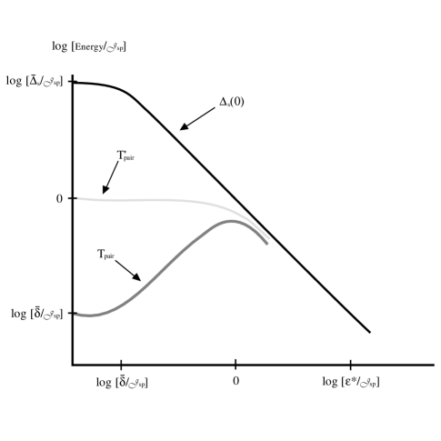
FIG. 2.: Energy scales from the solution of the pseudospin model as a function of $\varepsilon^{*}$: $\bar{\delta}$ and $\bar{\Delta}_{s}$ are, respectively, the coherence scale and the spin gap derived from the exact solution of the model for $\varepsilon^{*}=0$ and given in Eqs. (48) and (51), $\Delta_{s}(0)$ is the zero temperature value of the spin gap, $T_{pair}$ is the temperature scale at which $\Delta_{s}(T)$ begins to fall significantly relative to its zero temperature value, and $T_{pair}^{\prime}$ is the temperature at which $\Delta_{s}(T)\sim T$.

A For the case $\varepsilon^{*}\ll{\cal J}_{sp}[{\cal J}_{sp}/W]^{1/3}$,                                                i.e. when $\varepsilon^{*}\ll\bar{\delta}$

In this regime, the results are qualitatively the same as for $\varepsilon^{*}=0$. (Note that for $\varepsilon^{*}=T=0$, the self-consistent equations (99-103) are exact.) There is little temperature dependence of any of the gap parameters in the low temperature regime, $T\ll T_{pair}$, where

$$T_{pair}\sim\bar{\delta}.$$ (104)

Clearly, substantial suppression of $\Delta_{s}(T)$ due to pseudospin fluctuations begins to occur when $T\sim T_{pair}$; as a consequence, $T_{pair}/\Delta_{s}(0)\sim\rho(E_{f})\Delta_{s}(0)\ll 1/2$.

There follows an intermediate temperature regime, $T_{pair}\ll T\ll T_{pair}^{\prime}$, where

$$T_{pair}^{\prime}\sim{\bar{\delta}_{s}}[{\bar{\Delta}}/{\bar{\delta}_{s}}]^{2(1-\alpha)/(2-\alpha)};$$ (105)

in this regime, even though $\Delta_{s}(T)$ is strongly suppressed, it is still true that $\Delta_{s}(T)\gg T$, so we can approximate $<\cos[\sqrt{2\pi}\phi_{s}]>$ by its zero temperature value Eq.(103), with the consequence that

$$\Delta_{s}(T)\approx{\bar{\Delta}_{s}}[\beta{\bar{\delta}}]^{\alpha/2(1-\alpha)}$$ (106)

and

$$\delta(T)\approx{\bar{\delta}}[\beta{\bar{\delta}}]^{{(2\alpha-1)}/{2(1-\alpha)}}.$$ (107)

However, while significant spin pairing still survives in this temperature range, the entropy of the pseudospins is recovered, and hence the specific heat, $C_{v}\sim[\delta(0)/T]^{1/(1-\alpha)}$, is large.

$T_{pair}^{\prime}$ is the temperature at which $T=\Delta_{s}(T)$, where $\Delta_{s}(T)$ is given by Eq. (106). For temperatures $T\gg T_{pair}^{\prime}$, there is no coherence, no apparent gap in any of the degrees of freedom, and the problem can be treated using a high temperature expansion.

We can summarize the heirarchy of scales in this case as

$${\bar{\Delta}_{s}}\sim\Delta_{s}(0)\gg T_{pair}^{\prime}\gg T_{pair}\sim\delta(0)\sim{\bar{\delta}}\gg\varepsilon^{*}.$$ (108)

Specifically, for the $\alpha=2/3$ case, ${\bar{\Delta}_{s}}\sim{\cal J}_{sp}^{2/3}$, $T_{pair}^{\prime}\sim{\cal J}_{sp}$, and ${\bar{\delta}}\sim{\cal J}_{sp}^{4/3}$.

B For the case ${\cal J}_{sp}[{\cal J}_{sp}/W]^{1/3}\ll\varepsilon^{*}\ll{\cal J}_{sp}\ \ \ \ \ \ \ \ \ \ \ \ \ \ \ \ \$ i.e. when ${\bar{\delta}}\ll\varepsilon^{*}\ll{\bar{\delta}_{s}}[{\bar{\Delta}}_{s}/{\bar{\delta}_{s}}]^{2(1-\alpha)/(2-\alpha)}$

It is easy to see from Eqs. (101) and (102) that larger values of $\varepsilon^{*}$ supress the thermal disordering of the pseudo-spins, and hence removes the anomalous renormalization of $\Delta_{s}(T)$ at low temperatures. At $T=0$, and so long as $\varepsilon^{*}\gg{\bar{\delta}}$,

$$\delta(0)=\bar{\delta}[{\bar{\delta}}/\varepsilon^{*}]^{1/2(1-\alpha)}$$ (109)

and

$$\Delta_{s}(0)={\bar{\Delta}_{s}}[{\bar{\delta}}/\varepsilon^{*}]^{(2\alpha-1)/2(1-\alpha)}.$$ (110)

If at the same time, $\varepsilon^{*}\ll T_{pair}^{\prime}$, then $\Delta_{s}(0)\gg\varepsilon^{*}$, so

$$T_{pair}\sim\varepsilon^{*}.$$ (111)

For $T\ll T_{pair}$, there is little temperature dependence of the gaps, whereas, for $T\gg T_{pair}$, $\varepsilon^{*}$ falls out of the problem so $\Delta_{s}(T)$, $\delta(T)$, and $T_{pair}^{\prime}$ are given by Eqs. (106), (107), and (105), as before.

The remarkable property of this range of parameters is that, as $\varepsilon^{*}$ increases, the spin gap at $T=0$ decreases rapidly (as expected) but the pairing temperature, $T_{pair}$ actually increases. In other words, in order to obtain a high temperature scale for pairing, the charge transfer energy, $\varepsilon^{*}$, should be somewhat above the Fermi energy!

We can summarize the heirarchy of scales in this case as

$${\bar{\Delta}_{s}}\gg\Delta_{s}(0)\gg T_{pair}^{\prime}\gg T_{pair}\sim\varepsilon^{*}\gg{\bar{\delta}}\gg\delta(0).$$ (112)

One remarkable feature of this result, which relies on the particular value $\alpha=2/3$, is that in this regime $\Delta_{s}(0)\sim[{\cal J}_{sp}]^{2}/\varepsilon^{*}$, $T_{pair}\sim\varepsilon^{*}$, and $T_{pair}^{\prime}\sim{\cal J}_{sp}$ are all independent of the bandwidth. Note that at the upper end of this range, $\Delta_{s}(0)\sim T_{pair}\sim T_{pair}^{\prime}\sim\varepsilon^{*}\sim{\cal J}_{sp}$! This same conclusion follows from evaluating the expressions in the next subsection at the lower limit of the stated range.

C For the case ${\cal J}_{sp}\ll\varepsilon^{*}\ll W$,                                                        i.e. when ${\bar{\delta}}[{\bar{\Delta}_{s}}/{\bar{\delta}}]^{2(1-\alpha)/(2-\alpha)}\ll\varepsilon^{*}\ll W$

Whenever ${\bar{\delta}}[{\bar{\Delta}_{s}}/{\bar{\delta}}]^{2(1-\alpha)/(2-\alpha)}\ll\varepsilon^{*}$, it follows that $\Delta_{s}(0)\ll\varepsilon^{*}$. As a consequence, the temperature dependence of the various gaps is set by

$$T_{pair}\sim\Delta_{s}(0)$$ (113)

where $\Delta_{s}(0)$ and $\delta(0)$ are given by Eqs. (90) and (109), above; moreover, there is no longer a distinct temperature scale $T_{pair}^{\prime}$.

The heirarchy of scales in this case can be summarized as

$${\bar{\Delta}_{s}} \gg\Delta_{s}(0)\sim T_{pair}\gg{\bar{\delta}}\gg\delta(0),$$ (114)

$$\varepsilon^{*} \gg\Delta_{s}(0).$$ (115)

In this regime, both $\Delta_{s}(0)$ and, correspondingly, $T_{pair}$ are decreasing functions of $\varepsilon^{*}$. To be specific, for the case of $\alpha=2/3$, $T_{pair}\sim{\cal J}_{sp}^{2}/\varepsilon^{*}$ and $\delta(0)\sim T_{pair}\sqrt{\varepsilon^{*}/W}$.

D $\varepsilon^{*}\sim W$: Renormalized interactions

In the limit of large $\varepsilon^{*}$, the dynamical nature of the collective mode is unimportant; it could have been integrated out to obtain new effective interactions in the 1DEG, with retardation and spatial non-locality limited by the size of $\varepsilon^{*}$. Moreover, since in this limit, holon pairs in the environment exist only as dilute, virtual excitations, it is sufficient to compute these interactions perturbatively in powers of ${\cal J}_{sp}/\varepsilon^{*}$. To second order in ${\cal J}_{sp}$, the Hamiltonian is of the same form as $H_{1DEG}$ in Eq. (2), but with a renormalized chemical potential and interactions:

$$g_{1}^{*}=g_{1}-\delta g.$$ (116)

$$K_{s}^{*}=K(g_{1}^{*})$$ (117)

$$v_{s}^{*}=v_{s}+\delta g/2\pi,$$ (118)

where $\delta g=({\cal J}_{sp})^{2}/4\varepsilon^{*}$.

When $g_{1}$ is small, $g_{1}^{*}<0$ and the pair fluctuations produce a net attractive interaction in the spin degrees of freedom, which leads to a spin gap of magnitude[74]

$$\Delta_{s}=4\sqrt{2\lambda/\pi}(v_{s}/a)\exp[-1/\lambda]$$ (119)

where $\lambda=\rho_{s}|g_{1}^{*}|/a$ and $\rho_{s}=a/\pi v_{s}$. It is also clear that there is a corresponding crossover temperature, $T_{pair}\approx\Delta_{s}/2\ll\varepsilon^{*}$, above which the spin gap vanishes and the spin excitations are well described as linearly dispersing collective modes with velocity $v_{s}^{*}$. Again, the charge modes are completely unaffected by the pairing physics, and so continue to be described as linearly dispersing modes with velocity $v_{c}$. Hence the Drude weight (or, equivalently for the 1DEG, the zero temperature superfluid phase stiffness ) is unrenormalized.

This analysis is strictly correct only if $\varepsilon^{*}>W$, because it did not take account of retardation, which implies that the induced interaction $\delta g_{1}$, vanishes for energy exchange much greater than $\varepsilon^{*}$. However, for the physically more interesting case, $W\gg\varepsilon^{*}\gg{\cal J}_{sp}$, the effect of retardation can be studied using an energy shell renormalization group scheme, as in the electron-phonon problem[20]. This improved treatment produces results that are similar in spirit to those described above, except that, for energies smaller than $\varepsilon^{*}$ (when there is no longer a distinction between the retarded and instantaneous pieces of the interaction), the effective interaction has a renormalization, $\delta g_{1}$, which is a complicated, but calculable[20], function of $g_{1}$, $({\cal J}_{sp})^{2}/4\varepsilon^{*}$, and $\varepsilon^{*}/W$. In all cases, there is a critical value of the charge transfer energy $\varepsilon_{c}\sim({\cal J}_{sp})^{2}/4g_{1}$, such that for larger $\varepsilon^{*}>\varepsilon_{c}$, the renormalized value of $g_{1}$ is positive at low energies, and there is no spin gap, whereas for $\varepsilon^{*}<\varepsilon_{c}$, $g_{1}^{*}$ is negative and a spin gap opens up at zero temperature. This answers the question of how “active” the environment must be.

E Effects of “irrelevant” interactions

We now consider the effects of various interactions that we set equal to zero in the decoupling limit. Because the spectrum of the pseudospin model has a gap at the solvable point, all of the omitted terms are formally irrelevant in the renormalization group sense. Of course this does not give us license to completely ignore these terms; they can have large quantitative, and at times qualitative effects on the physics of interest, even if they do not affect the character of the true asymptotic behavior of the system.

Let us consider the effects of non-zero $\Delta V$ and, $\varepsilon^{*}$ on the nature of the excitations of the system at zero temperature. When these couplings are small, their most important qualitative effect is to induce dynamics for the pseudospins. In the presence of these terms, the effective Hamiltonian for the pseudospins, obtained by integrating out the electronic degrees of freedom[70], is qualitatively similar to (but not precisely equal to) the spin 1/2 Ising model in a transverse magnetic field,

$$H^{eff}\sim \sum_{R}[(\bar{\delta}/2)\tau_{R}^{x}+\varepsilon^{*}\tau_{R}^{z}]$$ (120)

$$- \sum_{R>R^{\prime}}[K(R-R^{\prime})\tau_{R}^{x}\tau_{R^{\prime}}^{x}+\tilde{K}(R-R^{\prime})\tau_{R}^{z}\tau_{R^{\prime}}^{z}]$$ (121)

in which $K(R-R^{\prime})\sim\bar{\delta}^{2}/\bar{\Delta}_{s}$ and $\tilde{K}(R-R^{\prime})\sim(\Delta V)^{2}/\bar{\Delta}_{s}$ and both have range of order $\xi_{s}$. As is well known, a transverse field induces dynamics (propagation of the kinks) in the spin 1/2 Ising model.

As we have seen, the other effect of $\varepsilon^{*}$ is to supress thermal fluctuations of the pseudospins. At high temperatures, there is an entropy density $S=(a/\xi_{p})\ln\ 2$ associated with the discrete symmetry of the pseudospins. For $\varepsilon^{*}=0$, this entropy is lost at about the temperature $T_{pair}\sim\bar{\delta}$, where strong pairing sets in. In higher dimensional systems this large entropy is presumably responsible for heavy-fermion behavior in the model[4]; in the present context it leads to the small ratio of $T_{pair}/\Delta(0)$. When $\varepsilon^{*}>\bar{\delta}$, the majority of the entropy associated with the pseudospins is lost at temperatures greater than $T_{pair}$. As a consequence, thermal disordering effects are relatively less severe, and $T_{pair}/\Delta(0)\sim 1/2$ is rapidly restored.

VII The Behavior of the Charge Degrees of Freedom:

We have seen that, in the pseudospin model, the canonical tranformation decouples the charge degrees of the 1DEG from the environment, and their fluctuations are described by the quadratic Hamiltonian, ${\cal H}_{c}^{0}$. This Hamiltonian describes a fluctuating superconductor, with phase $\theta_{c}$, or in dual language, a fluctuating charge density wave, with phase $\phi_{c}$. Evidently, proximity to commensurability or the existence of an external potential can substantially modify the physics.

A The role of Umklapp scattering

The charge fields of the 1DEG are governed by the Hamiltonian:

$$\tilde{H}_{c}=H_{0}^{c}+H_{1}^{c},$$ (122)

where $H_{0}^{c}$ and $H_{1}^{c}$ are given in Eqs.(39) and (40). Now the $c$-number $(4k_{F}-G)x$ may absorbed into the phase $\phi_{c}$, without changing the commutation relations and the quadratic part of $H_{0}^{c}$ in Eq. (39) may be diagonalized by the canonical transformation $\phi_{c}\rightarrow\phi_{c}K_{c}^{1/2}$, $\Pi_{c}\rightarrow\Pi_{c}/K_{c}^{1/2}$. The net result is that the charge degrees of freedom are described by a sine-Gordon model with a chemical potential $\mu^{*}$ given by

$$\mu^{*}={v_{c}(4k_{F}-G)\over 4K_{c}}.$$ (123)

For the strongly incommensurate case, in which $\mu^{*}$ is large, we can ignore the umklapp scattering term (proportional to $g_{3}$); in this case the charge excitations are gapless collective modes with a sound-like dispersion and a velocity, $v_{c}$, that is unrenormalized by the interactions with the environment. Correspondingly, the Drude weight, or superfluid phase stiffness (which cannot be distinguished in one dimension in the absence of disorder) are also unrenormalized.

In the nearly commensurate case, which characterizes the doped-insulator region, the analysis of the corresponding sine-Gordon theory is the same as for the spin degrees of freedom. In particular, for $K_{c}<1$, which is always satisfied for repulsive interactions, the “particles” in the theory are massive solitons with charge e and spin 0. It follows at once that the system undergoes an insulator to metal transition at $|\mu^{*}|=\Delta_{c}$, where the chemical potential moves out of the gap, and that there is a finite density of solitons:

$$n_{sol}={\sqrt{(\mu^{*})^{2}-\Delta_{c}^{2}}\over\pi v_{c}}$$ (124)

with $\mu^{*}$ given in Eq. (123). For small $n_{sol}$, the Drude weight of the stripe is proportional to $n_{sol}$. This argument is similar to the analysis of the commensurate-incommensurate transition by Pokrovsky and Talapov [75], except that they considered a two-dimensional classical problem, equivalent to the quantum sine-Gordon problem in imaginary time.

For quarter-filled stripes [76], $4k_{F}=2\tilde{k}_{F}=G/2$, so the charge density on the stripe and in the environment may jointly lock to the lattice. This commensurability effect competes with superconductivity but, if the coupling constant is not too large, it may not develop beyond the logarithmic temperature dependence that characterizes the early stages of renormalization[77]. We are investigating this behavior as a potential source of the special stability of quarter-filled stripes for doping $x<1/8$ in the La₂CuO₄ family[41, 78], and the logarithmic temperature dependence of the resistivity observed [79, 41] when the onset of superconductivity is suppressed.

B External Periodic Potential

Here it is assumed that there is an external potential with a wave vector $q$ which is close to $2k_{F}$. Then the Hamiltonian must be supplemented by a contribution

$$H_{e}=u\sum_{\sigma}\int_{-\infty}^{\infty}dx[\psi^{\dagger}_{1,\sigma}\psi_{2,\sigma}e^{i(2k_{F}x-qx)}+H.c.],$$ (125)

which may be written in the boson representation (21) as:

$$H_{e}={2u\over\pi a}\int dx\ \ cos\bigg{[}\sqrt{2\pi}\phi_{c}+(q-2k_{F})x\bigg{]}cos\bigg{[}\sqrt{2\pi}\phi_{s}\bigg{]}.$$ (126)

It is straightforward to show that, when the pseudospin representation is introduced for the charge degrees of freedom of the environment, then $H_{e}$ is not changed by the unitary transformation defined by $U$ in Eq. (48): i.e. $U^{\dagger}H_{e}U=H_{e}$. Moreover, it is clear from the spin Hamiltonian (84) that $cos[\sqrt{2\pi}\phi_{s}(x)]$ has a finite expectation value so that it may be replaced by a constant in $H_{e}$ to obtain the asymptotic behavior of the charge degrees of freedom. Umklapp scattering may be ignored if it is an irrelevant variable or if $4k_{F}$ is sufficiently far from a reciprocal lattice vector. However, the effect of the periodic potential is similar to that of umklapp scattering. The main differences are that the solitons are massive when $K_{c}<4$, (as opposed to $K_{c}<1$ for umklapp scattering) and that $\mu^{*}=v_{c}(2k_{F}-q)/K_{c}$, which modifies the condition for the metal-insulator transition.

The physical argument for including such a potential is as follows: In the ordered state of La_1.6-xNd_0.4Sr_xCuO₄, the holes on a given stripe move in an effective potential produced by the stripes in a neighboring CuO₂ plane. Since stripes in adjacent planes are perpendicular to each other, the wave vector of the charge contribution to the effective potential is given by $q=2\epsilon$ in units of $2\pi/a$, where $a$ is the lattice spacing [41]. In the same units, $2k_{F}=n_{s}/2$, where $n_{s}$ is the concentration of doped-holes on a given stripe. The present experimental evidence [41, 42] is consistent with $\epsilon=1/8$ and $n_{s}=1/2$ and hence $q=2k_{F}$ for dopant concentration $x=1/8$. This is the hole concentration near which the superconducting $T_{c}$ is suppressed in the stripe-ordered material La_1.6-xNd_0.4Sr_xCuO₄ [80] and in La_2-xBa_xCuO₄, for which there is indirect evidence of stripe order [81].

An array of stripes will undergo a transition to a superconducting state at a temperature which is determined by the onset of phase coherence and is proportional to the superfluid phase stiffness [8] which, in turn, is proportional to $n_{sol}$.

In Sec. III we considered the case in which the environmental spin gap arose because the backscattering term proportional to $\tilde{g}_{1}$ was relevant. For a half-filled band with $\tilde{g}_{3}$ also relevant, there is a broken symmetry ground state with period 2$a$, which produces an external potential on the stripe, with a wave vector equal to 4$k_{F}$ when $n_{s}=1/2$. Such a potential is commensurate with the umklapp term $g_{3}$, so the coupling between these terms must be taken into account. This is an example in which spin gaps with and without a broken symmetry may lead to different consequences. The physical case has no broken symmetry.

VIII Spin Gap Center

Another model of some physical interest has a spin gap at one specific location as, for example, at an isolated antiferromagnetic region in a metal. This is an example of a dynamical impurity problem, in which the conduction electrons couple to a center with internal degrees of freedom. It is well known that an angular momentum analysis produces a one-dimensional Hamiltonian involving the radial motion of incoming and outgoing fermions on the half line $r>0$, where $r$ is the distance from the pairing center [60]. Also, it is possible to extend the space to all values of $r$ by transforming incoming fermions for $r>0$ to incoming fermions at position $-r$. Then the problem is formally equivalent to a one-dimensional electron gas in which only the right-going fermions interact with the pairing center. In the absence of left-going fermions, the operator $P^{\dagger}$, introduced in Eq. (17), cannot be defined and only the $\eta$-pairing term [82]

$$P^{\dagger}_{\eta,1}=\psi_{1,\uparrow}^{\dagger}\psi_{1,\downarrow}^{\dagger},$$ (127)

couples to the pairing center. Triplet pairing terms are omitted because the exclusion principle requires them to be of the form $\psi^{\dagger}_{1,\uparrow}\partial\psi^{\dagger}_{1,\uparrow}$ which is less relevant than $P^{\dagger}_{\eta,1}$. (The derivative in the triplet operator leads to an extra power of $1/x^{2}$ in the correlation function.) Thus a pairing center naturally produces singlet pairing.

We consider the case in which the center has a large spin gap, so the pseudospin variable (representing charge transfer to the center) is the only internal degree of freedom of the center that we retain, explicitly. Thus the Hamiltonian is

$$H_{center}=H_{1DEG}+H_{\eta}$$ (128)

where $H_{1DEG}$ is given in Eq. (2), although in the case in which the metallic degrees of freedom represent a higher dimensional Fermi liquid, one must set the interactions ($g_{a}$) to zero. The bosonized form of $H_{\eta}$ is

$$H_{\eta} =\varepsilon\tau^{z}+{V\over\sqrt{2}\pi}\tau^{z}\Phi_{c}^{\prime}(0)$$ (129)

$$+ \frac{{\cal J}_{\eta}}{\pi a}\big{[}\tau^{-}e^{i\sqrt{2}\Phi_{1,c}(0)}+H.c.\big{]}.$$ (130)

Here $\Phi_{1,c}(0)=[\Phi_{1,\uparrow}(0)+\Phi_{1,\downarrow}(0)]/\sqrt{2}$. In this form the model is equivalent to a single-channel Kondo problem [60], and it may be solved by making a unitary transformation $H_{center}\rightarrow U^{\dagger}H_{center}U$ with

$$U=exp[-i\lambda\Phi_{c}(0)\tau^{z}]$$ (131)

and choosing $\lambda=\sqrt{2}-1$, for the special point $V=\sqrt{2}\pi\lambda v_{c}$. Then $\tilde{H}_{center}$ becomes

$$U^{\dagger}H_{center}U =H_{1DEG}+\varepsilon\tau^{z}$$ (132)

$$+ \frac{J}{\pi a}\big{[}\tau^{-}e^{i\Phi_{1,c}(0)}+H.c.\big{]}$$ (133)

This the Hamiltonian may be “refermionized” by writing the pseudospin operator in the form $\tau^{+}=\eta d$ where $\eta$ is an anticommuting $c$-number and $d$ is a fermion annihilation operator, and inverting the boson representation of fermion fields:

$$\psi_{c}^{\dagger}=\eta{e^{i\Phi_{c}}\over\sqrt{2\pi a}}.$$ (134)

When written in terms of these variables, the right-going part of the Hamiltonian becomes

$$U^{\dagger}H_{1,center}U= -iv_{c}\int_{-\infty}^{\infty}dx\big{[}\psi^{\dagger}_{c}\partial_{x}\psi_{c}]$$ (135)

$$+ {{\cal J}_{\eta}\over\sqrt{2\pi a}}(d\psi^{\dagger}_{c}(0)+H.c.),$$ (136)

which is precisely the Toulouse limit from which all of the well-known behavior of the single channel Kondo problem may be derived [60]. This argument strongly suggests that arrays of pairing centers in two and three dimensions behave like Kondo lattices, and that they should show heavy-Fermion behavior [4].

Of course a single pairing center in a purely one-dimensional model should also exhibit this single-channel Kondo behavior. This would not happen if we replaced the pseudospin array in Eq. (78) by a single center, because we would have omitted a possible $\eta$-pairing interaction, of the form ${\cal J}_{\eta}\tau_{R}^{+}[P_{\eta,1}+P_{\eta,2}]$ in that Hamiltonian. While momentum conservation indeed makes this term unimportant for the extended array, a spin-gap center, by its very nature, breaks translational symmetry and hence permits finite momentum transfer scattering processes. Including these terms, the total pair coupling at a single spin-gap center in Eq. (17) may be written

$$H_{pair} = \big{\{}{\cal J}_{sp}P^{\dagger}(R)$$ (137)

$$+ {\cal J}_{\eta}[P_{\eta,1}(R)e^{2ik_{F}R}+P_{\eta,2(R)e^{-2ik_{F}R}}]\big{\}}\tau^{-}_{R}+{\rm H.c.}.$$ (138)

If we consider a single center at $R=0$, and consider the case ${\cal J}_{\eta}=0$, the left-going fermions at position $x$ may be transformed to right-going fermions at position $-x$, without changing the Kondo coupling. Thus the subscripts 1,2 become “flavor” labels and we have a two-channel Kondo problem. However, in this language, the ${\cal J}_{\eta}$ term breaks the “channel degeneracy”, and is pertubatively relevant, so it produces a single-channel Kondo problem. On the other hand the oscillating factors in Eq. (137) make the ${\cal J}_{\eta}$ perturbatively irrelevant for the array and moreover, since the mismatch of momenta between the 1DEG and the antiferromagnet imply that ${\cal J}_{\eta}$ is small compared to ${\cal J}_{sp}$, the neglect of $\eta$-pairing interactions for the extended system is justified. This is analagous to the behavior found previously for Kondo systems[49], where the anisotropic single-channel Kondo array, behaves as if it were a two-channel Kondo array, even though the single impurity version of the model exhibits ordinary Kondo behavior.

IX Discussion

A Summary of results

We have studied a model of a 1DEG in an active environment, focussing in particular, on the case in which the environment possesses both a charge gap and a spin gap, and the energy difference between a singlet pair of holes in the 1DEG and the environment, $\varepsilon$, is small in comparison to the bandwidth. We have discovered a new mechanism for producing strong superconducting fluctuations on a high temperature scale, in which a spin gap is induced in the regions between the stripes by spatial confinement, and transferred to the 1DEG by pair tunnelling. A striking feature of this mechanism of superconductivity, which may be described as a spin-gap proximity effect, is that the pairing (i.e. the spin gap) is a property of the insulating state itself, and it is simply imprinted on the mobile holes through their virtual excursions into the insulating regions. We have found that this phenomenon is robust and, in particular, it survives the presence of strongly repulsive forward scattering interactions, i.e. Coulomb repulsion between electrons.

We have demonstrated that the physics of this problem is captured by a simple pseudospin model, for which exact and well-controlled approximate results can be obtained. This model includes the most important interactions: the renormalized pair-tunnelling matrix element, ${\cal J}_{sp}$ (defined in Eq. (85)), the renormalized energy cost, $\varepsilon^{*}$, required to move a singlet pair of holes from the 1DEG to the environment, the bandwidth of the 1DEG, $W\sim E_{F}$, (which is assumed to be large compared to other energies), and the exponent, $\alpha$, which characterizes the spin correlations of the 1DEG. We have used renormalization group arguments to show that $\alpha\approx 2/3$ for repulsive, spin-rotationally invariant interactions, and we shall use this value of $\alpha$ in discussing our results.

We have found that, generically, this model produces singlet pairing (spin gap behavior) at a high temperature, $T_{pair}$: in the limit $\varepsilon^{*}\rightarrow 0$, $T_{pair}\sim{\cal J}_{sp}({\cal J}_{sp}/W)^{1/3}$, while for $\varepsilon^{*}\gg{\cal J}_{sp}({\cal J}_{sp}/W)^{1/3}$, $T_{pair}$ is the smaller of $\varepsilon^{*}$ and $\Delta_{s}(0)\sim{\cal J}_{sp}^{2}/\varepsilon^{*}$. Remarkably, this means that for small $\varepsilon^{*}$, $T_{pair}$ is an increasing function of $\varepsilon^{*}$, which reaches a maximum value of $T_{pair}\sim{\cal J}_{sp}$ when $\varepsilon^{*}\sim{\cal J}_{sp}$. Below $T_{pair}$, singlet superconducting and CDW susceptibilities diverge as $T\rightarrow 0$, with the stronger divergence typically associated with the CDW. Moreover, this high pairing scale is not accompanied by any significant reduction of the zero temperature superfluid phase stiffness (Drude weight), i.e. there is no strong mass renormalization. We have also identified a zero-temperature spin gap energy, $\Delta_{s}(0)$, which plays the role of the superconducting gap, $\Delta_{0}$. In the small $\varepsilon^{*}$ limit the ratio $T_{pair}/\Delta_{s}(0)\sim\Delta_{s}(0)/W<<1/2$, while for large $\varepsilon^{*}$, $T_{pair}/\Delta_{s}(0)\approx 1/2$, as in BCS theory. (The evolution of these energy scales as a function of $\varepsilon^{*}$ is shown in Fig. 2, and discussed in Sec. VI.) The ground state of this model has a broken, discrete Z(2) symmetry, unrelated to any of the usual space-time symmetries of the problem, and a corresponding non-local order parameter which develops a non-zero expectation value in the ground state, and has an exponentially long correlation length at low temperatures. (See discussion of “$\tau$” symmetry in Appendix B.)

B Interactions Between Stripes and Possible Ordered Phases

To extend our results to situations in which there is a true phase transition, we must consider the properties of an array of one-dimensional systems (stripes). To avoid misunderstanding, we emphasise that, for purposes of the present discussion, “CDW” refers to charge ordering along the stripe direction, whereas “stripe order” implies charge ordering in the direction perpendicular to the stripes, i.e. ordering of the stripe positions and orientations. Of course, both types of order are a form of generalized charge density wave.

The ultimate nature of the long-range order depends, among other things, on the coupling between stripes, which is profoundly influenced by the intervening antiferromagnetically-correlated regions and, in particular, by the frustration of hole motion in the antiferromagnet, which was the driving force for the formation of the stripes themselves. Thus, this coupling should be smaller than the characteristic energies of the electronic correlations along the stripe, considered in this paper.

With this in mind, the onset of superconductivity in a dilute stripe array can be studied by introducing weak interactions between well-separated stripes. Single-particle tunnelling between stripes is an irrelevant perturbation [83], because of the existence of a spin gap, so we do not expect a crossover to higher-dimensional Fermi liquid behavior in this limit. Then the nature of the long-range order is determined by pair tunnelling and the Coulomb coupling between stripes.

Effects of Disorder: There are two distinct types of disorder which have very different effects on the physics of an array of stripes. The first is a degree of randomness in the couplings between stripes, which may be produced by impurities (as in e.g. organic conductors) or by quantum or thermal fluctuations in the stripe configuration. For a “self-organized” quasi one-dimensional system, such as a charged stripe array, the latter source of disorder is likely to be the more important. Disorder of this type favors superconductivity (which is a $k=0$ order) since it strongly frustrates the short-wavelength CDW order associated with the $4k_{F}$ or $2k_{F}$ instabilities of the 1DEG. This is especially so when the stripes are strongly fluctuating. In the simplest situation, the dynamics of the stripes is slow compared to the Josephson plasma frequency, as for example in La_2-xSr_xCuO₄, and the disorder is essentially static. On the other hand, if the CDW and superconducting fluctuations are on similar time scales, new physics may emerge; an interesting possibility is that there exists a novel quantum critical point which controls the physics in some region of temperatures and dopant concentration [84].

The second type of disorder affects the coherence of electronic motion along a single stripe. For a single stripe, the back scattering of holes from an impurity is always pertubatively relevant for the range of interactions considered here, because CDW correlations are enhanced[85]. However, the localization can be superseded by sufficiently strong Josephson coupling (pair-tunnelling) between stripes, and there will be an insulator to superconductor transition as the concentration of stripes grows or the Josephson coupling between stripes is, in any other way, increased, with fixed disorder. This is in agreement with the evolution of the ground state observed in La_2-xSr_xCuO₄ as a function of doping [78], or applied magnetic field[79].

Symmetry of the order parameter: If stripe order breaks the four-fold rotational symmetry of the crystal, the superconducting order will have [86, 87] strongly mixed extended-$s$ and $d_{x^{2}-y^{2}}$ symmetry! This will happen in a stripe-ordered phase, such as in La_1.6-xNd_0.4Sr_xCuO₄, or in a possible “stripe nematic” phase, in which the stripe positional order is destroyed by quantum or thermal melting or quenched disorder, but the stripe orientational order is preserved. (Such phases also would be characterized by large induced asymmetries in the electronic response in the $ab$-plane. Below we discuss some preliminary evidence for a transition to a stripe nematic phase in overdoped YBa₂Cu₃O_7-δ.)

On the other hand, when the stripes are disordered at long length scales, the thermodynamic distinction between $s$-wave and $d$-wave superconducting order is well defined; however, even here, if there is substantial orientational order to the stripe fluctuations at intermediate length scales, the interplay between the two types of superconducting order is likely to be more complicated and more subtle than in conventional, homogeneous materials. For example, one can imagine that, even in a phase which is globally $d$-wave, substantial mixtures of $s$ and $d$-wave order could occur over mesoscopic scales near surfaces[88] or twin boundaries.

Superconducting fluctuations: A necessary corollary of the stripe model is that, in lightly doped materials, the temperature scale, $T_{pair}$, at which pairing occurs (on a single stripe) is parametrically larger than the superconducting transition temperature, $T_{c}$, which is governed by the Josephson coupling between stripes. Moreover, since the pairing force derives from the local antiferromagnetic correlations in the regions between stripes, both $T_{pair}$ and $T_{c}$ must be less than the temperature scale, $T_{AF}$, below which local antiferromagnetic correlations develop. A sequence of crossovers is, indeed, observed experimentally in underdoped high temperature superconductors, and they have tentatively been identified[89] with these two phenomena; see Fig. 1, above, and the discussion below.

C Phase diagram of the high temperature superconductors

The schematic phase diagram shown in Fig. 1, shows the global framework in which our model is related to the properties of the high temperature superconductors. The axes in this figure are temperature, $T$, and doping concentration, $x$; hatched lines indicate the most important crossover temperatures, and the solid lines represent phase transitions to the antiferromagnetically ordered state at very small $x$, and to the superconducting state at larger $x$. (In general, there are additional phase transitions and possibly other crossovers, but here we wish to focus only on the central physical issues.)

The upper crossover temperature $T^{*}_{1}$ characterizes the aggregation of charge (holes) into stripes; as we have shown elsewhere, the driving force for this crossover is frustrated phase separation [14, 15, 16]. Above $T^{*}_{1}$ the holes are more or less uniformly distributed, and randomly disrupt antiferromagnetic correlations, while below $T^{*}_{1}$, the self-organized stripe array allows local antiferromagnetic correlations to develop in the hole-free regions of the sample. At short distances, low energy spin fluctuations should come from regions with the character of odd-leg ladders, and be like those of the one-dimensional Heisenberg model [22], and, indeed, there is experimental evidence [90] indicating that this is the case in La_2-xSr_xCuO₄. As $x\rightarrow 0$, $T^{*}_{1}$ approaches the temperature $T_{\chi}$ at which local antiferromagnetic correlations develop in the undoped systems[91]. Between $T^{*}_{1}$ and the superconducting transition temperature $T_{c}$, there is a large range of temperatures in which there are significant stripe correlations, but coherence between stripes can be largely ignored; this is the region of temperatures addressed by the calculations in this paper. As the concentration of holes increases, the separation between stripes eventually becomes comparable to their width, at which point all information concerning the Mott insulating state is lost; for this reason, we have shown $T^{*}_{1}\rightarrow 0$ at a dopant concentration, $x_{max}$.

We identify the lower crossover temperature $T^{*}_{2}$ with $T_{pair}$, the temperature at which pairing (spin gap) behavior emerges within a stripe. This is also the temperature below which significant local, quasi one-dimensional superconducting fluctuations become significant. For local probes of the spin and quasiparticle response functions, the system should appear all but superconducting below this temperature. Since $T_{pair}$ is more or less a property of a single stripe, we have shown it as a relatively insensitive function of $x$, until it is cut off by $T^{*}_{1}$ at larger dopant concentrations. From this figure, it is clear that $T_{pair}$ is substantially greater than $T_{c}$ throughout the underdoped regime, and possibly even at optimal doping, and only approaches closely to $T_{c}$ in the overdoped regime. Thus, in underdoped materials, $T_{c}$ is determined by the superfluid phase stiffness, and hence by the Josephson coupling between stripes, rather than by the pairing scale. This is consistent with our previous analysis[8].

It should be noted that a phase diagram of the same form as that shown in Fig. 1 has been considered, previously, on purely phenomenological grounds[89], with the crossover temperatures determined as follows:

1) The upper crossover occurred at a characteristic temperature deduced by Batlogg and coworkers[91] from an analysis of susceptibility and transport properties, and by Loram and coworkers[92] from an analysis of thermodynamic data. We feel that all of these phenomena are broadly consistent with our identification of $T^{*}_{1}$ with the emergence of stripe and local antiferromagnetic order. (It appears that a pseudogap appears in the c-axis optical conductivity[93] at this temperature. Much of the c-axis optical oscillator strength will be shifted to energies higher than $\tilde{\Delta}_{s}+\varepsilon^{*}/2$ as the stripe correlations emerge below $T^{*}_{1}$.) If we accept this identification, then for moderate doping concentrations, a typical value is $T^{*}_{1}\sim 300K$, although it depends somewhat on the particular material, and rather more strongly on the dopant concentration. Indeed, stripe correlations have been seen neutron scattering experiments all the way up to 300K, although the scattering cross section decreases continuously, making it difficult to identify them unambiguously at high temperatures[90].

2) The lower crossover was identified by Batlogg and Emery [89] as the characteristic “pseudogap” temperature, deduced from the temperature dependence of the Cu NMR $1/T_{1}T$, which correlates well with the emergence of superconducting gap structure in ARPES experiments [94, 95], and a narrowing of the “Drude-like” peak in the optical conductivity in the $ab$-plane[96]. If we accept this identification then, for moderate doping, $T_{pair}\sim 150K$, again depending somewhat on the particular material being studied.

D Relation to experiments

1 Estimates of the model parameters

To begin with, it is necessary to estimate the values of the important interactions which determine the behavior of the model. The physics is driven by the local antiferromagnetic correlations between spins, so a priori we expect the interactions, other than those within a single stripe, to be some fraction of $J_{AF}$, which in the high temperature superconductors is in the range $1000K-2000K$ [40]. For similar reasons, the bandwidth in the environment, $\tilde{W}$, is expected to be a few times $J_{AF}$; numerical simulations for the square lattice lead to the estimate that the hole bandwidth [97] is approximately $2.2J_{AF}$. On the other hand, a naive estimate of the bandwidth $W$ of the 1DEG is given by the bare value, $2t\sim 1eV$, although this is certainly reduced substantially due to virtual (high energy) single-particle excursions into the environment, i.e. leakage of the hole wavefunction into the insulating neighborhood of the stripe.

More detailed estimates may be obtained from experiment. Since $\varepsilon^{*}/2$ is the binding energy of a holon in the stripe, we expect that it also determines the temperature at which stripes begin to lose their integrity, so we estimate that $\varepsilon^{*}\sim 2T^{*}_{1}$. Thus, $\varepsilon^{*}$ is certainly remarkably small, $\varepsilon^{*}\sim J_{AF}/2$, but still large enough that the peculiarities of the small $\varepsilon^{*}$ limit are avoided. Similarly, if we identify $T_{pair}$ with the spin-gap temperature deduced from NMR, we can approximately invert the relation $T_{pair}\sim{\cal J}_{sp}^{2}/\varepsilon^{*}$ to obtain an estimate of ${\cal J}_{sp}\approx\varepsilon^{*}$, where the exact numerical relation between these two quantities depends on numerical amplitudes which we cannot calculate with any great accuracy. For this range of parameters, it also follows that $\Delta_{s}(0)\sim T_{pair}$, consistent with estimates of the superconducting gap from photoemission experiments. Finally, from the magnitude of the pseudogap observed in c-axis optical response, we estimate that $\tilde{\Delta}_{s}\approx\varepsilon^{*}$. This implies that the cuprates lie in the crossover region between large and small $\varepsilon^{*}$ (regimes B and C described in Sec. VI), which is also the region of maximum $T_{pair}$, as shown in Fig. 2. We feel that these values of $\varepsilon^{*}$, ${\cal J}_{sp}$, and $\tilde{\Delta}_{s}$ are physically reasonable.

2 Does local pairing on stripes provide a consistent explanation of the pseudogap behavior of underdoped cuprates?

In the above discussion, we interpreted the experimentally measured pseudogap behavior in underdoped cuprates as superconducting pairing in a large range of temperatures above $T_{c}$. This behavior was predicted by us[8] on the basis of a phenomenological analysis of the relation between the superconducting $T_{c}$ and the measured zero temperature superfluid phase stiffness (i.e. the zero temperature London penetration depth). It provides a very natural explanation of the “spin gap” behavior that has been widely observed in planar copper NMR measurements in underdoped cuprates[98]. Here, there is a peak in $1/T_{1}T$ at a characteristic pairing temperature above $T_{c}$, below which there is a rapid falloff that is quite similar to that observed below $T_{c}$ in more heavily doped cuprates. The interpretation of the spin gap as a superconducting gap has recently received considerable support from ARPES experiments[94, 95] which find that the magnitude and wave vector dependence of the pseudogap above $T_{c}$ is similar to that of the gap seen well below $T_{c}$ in both underdoped and optimally doped materials. The temperature above which this gap structure becomes unobservable correlates well with the pairing scale deduced from spin gap measurements. Measurements of the in-plane optical response are also highly suggestive of superconducting pairing above $T_{c}$ in underdoped cuprates[99, 100, 96].

This interpretation has been questioned because a large fluctuation diamagnetism and conductivity have not been observed between $T_{c}$ and $T_{pair}$ [101]. However, we believe that the absence of dramatic magnetic field effects is readily understood. Well above $T_{c}$, the superconducting fluctuations are essentially one dimensional, with little effect of the Josephson coupling between stripes. Consequently, an applied magnetic field does not drive any significant orbital motion until coherence develops in two (and ultimately three) dimensional patches, close to $T_{c}$. We are currently engaged in more detailed calculations of these effects, to make this argument more quantitative.

Recently it has been determined[78, 80] that in underdoped and optimally doped La_2-xSr_xCuO₄, there is a unique relation between the mean separation between stripes (i.e. the half-period of the dynamical incommensurate spin fluctuations) and the superconducting $T_{c}$. We have previously predicted such a relation[86] as a natural consequence of the existence of superconducting fluctuations on a single stripe and the idea that $T_{c}$ is determined by the Josephson coupling between stripes.

3 Commensurability and Near Commensurability Effects

The charge density on the stripes (and hence, the value of $k_{F}$) is largely determined by the competition between the local tendency to phase separation and the long-range Coulomb interaction; however, there are commensurability effects both within the 1DEG (which tend to pin $2k_{F}a=2\pi/m$ where $m$ is the order of the commensurability) and transverse to the stripes, which tend to pin the spacing between stripes at an integer times the lattice constant[16]. In La_2-xSr_xCuO₄, neutron scattering evidence supports the notion that there is a strong tendency toward locking the hole density within a stripe near commensurability $m=4$ for a range of $x$ less than $x=0.125$, and to pin the spacing between stripes near 4 lattice constants for $x>0.125$. (See Sec. VIIB.) Within the theory of the 1DEG, commensurability leads to a charge gap and insulating behavior. However, for a weak commensurability, the gap develops at low temperatures where it must compete with superconductivity. (For an alternative view, see Ref. [102].)

4 Are there any experimentally testable predictions that can be made on the basis of this mechanism?

To begin with, it is important to stress that there already exists considerable experimental evidence that the physics discussed in this paper is pertinent to the high temperature superconductors. Some of this has been discussed above. Neutron scattering and transport measurements provide direct evidence of hole-rich metallic stripes in an antiferromagnetic environment in at least the La₂CuO₄ family of materials. The convincing experimental evidence that underdoped cuprates behave like granular materials in that a superconducting gap opens well above $T_{c}$, strongly suggests that the superconductivity is inhomogeneous at some intermediate scale of length and time. Moreover, the absence of strong effects of magnetic fields in a regime of strong superconducting fluctuations indicates that these inhomogeneities are likely to be one-dimensional in character. The fact that both s-wave and d-wave symmetry are manifest in different phase-sensitive experiments on essentially the same materials supports the idea that there are strong, local fluctuations which break the (approximate) four-fold rotational symmetry of the crystal[103, 87].

However, while we feel that these experimental facts provide strong evidence for the general form of our model, they do not probe microscopic structure of the proposed pairing mechanism. There are, however, various signatures that could, in principle, be detected. We predict a spin-1, charge zero excitation (a quasi one-dimensional, magnon mode) with an energy gap $\Delta_{s}$, which is of order the superconducting gap. This mode could, in principle, be detected in neutron scattering. We also predict one or more gapped charge=0, spin=0 modes, the breathers; for the expected case of $\alpha=2/3$ there are two such modes, and the lowest energy one should also have energy gap $\Delta_{s}$. This mode could, in principle, be observed by Raman scattering[104]. Since it also could hybridize with a phonon, it could also show up in neutron scattering. It is interesting to note that a phonon mode which is sensitive to the onset of superconductivity, [104, 105] and a magnon, both with energy about 40meV have been observed[106] in the superconducting state of YBa₂Cu₃O_7-δ; we are currently exploring whether these two phenomena reflect the two collective modes discussed above.

A stripe structure may have a nematic phase, in which the stripes are orientationally ordered along a particular direction. Such a phase should display a striking anisotropy in its phase stiffness. It is interesting to note that a big increase in the phase stiffness is observed as YBa₂Cu₃O_7-δ is overdoped[107]. This behavior has been attributed to superconductivity (induced by the proximity effect) in the CuO chains, as they become filled. However, such an interpretation requires that the superfluid density in the chains is greater than in the planes, where it originated. Experimentally it may not be easy to distinguish nematic stripe order in overdoped YBa₂Cu₃O_7-δ given the existence of the CuO chains.

One feature of our model is that there are two, physically distinct, spin gaps, one associated with the 1DEG, and hence with the “superconducting gap”, and the other (larger gap) with the insulating environment. However, in practice, we expect that the two gaps will be similar in magnitude because the difference will be “smoothed out” by the motion of the holes between the stripe and the environment. (Exactly this sort of “smoothing out” of the gap occurs in the “Cooper limit” for the conventional proximity effect.) Finally, we observe that there are calculable consequences of our model for single particle properties, such as the density of states, which are currently under investigation.

Another qualitative test of our ideas is to look for high temperature superconductivity in new materials that have one-dimensional metallic and spin-gapped regions in close electrical contact built into their structure, and not necessarily self-organized. In this regard, we note that a material with even-leg undoped ladders (which have a spin gap[22]) in intimate contact with doped CuO₂ chains should display the mechanism of superconductivity that we have proposed here. Interestingly, superconductivity with $T_{c}=12K$ has been observed [108] at a pressure of 3GPa in Sr_0.4Ca_13.6Cu₂₄O_41.84, a material with this kind of structure, although the chains and ladders are in different planes, so the electrical conatct is not as strong as we would like. At atmospheric pressure, it appears that the doped holes are in the chains[109] but, at present, it is not known if this feature persists at the high pressures required for superconductivity.

Our model also could be studied by numerical techniques. In particular, an environment with a spin gap could be represented by either a two-leg ladder or an incommensurate dimerized half-filled chain. An environment without a spin gap would be a half-filled one-dimensional Hubbard model. In either case the coupling to the 1DEG should involve strong single-particle or pair hopping and a repulsive interaction between holes.

Acknowledgements: We would like to aknowledge important insights we have gained in discussions with D. Basov, R. C. Dynes, E. Fradkin, D-H. Lee, S. Sondhi, and J. Tranquada. SK would like to acknowledge the hospitality of the Physics Department at UC Berkeley, where this work was initiated, and the support of the Miller Foundation, through a Miller Visiting Professorship, and from a John Simon Guggenheim Foundation, Fellowship. This work was supported in part by the National Science Foundation grant number DMR93-12606 (SK) at UCLA. Work at Brookhaven (VE) was supported by the Division of Materials Science, U. S. Department of Energy under contract No. DE-AC02-76CH00016.

A Perturbative Renormalization Group Analysis

There are three related senses in which we use the renormalization group to analyze a complex physical problem, such as the present one.

1) Firstly, the renornmalization group, and in particular the notion of fixed points, is a theory of theories, and it provides a context and structure which allows the problem to be approached in the context of its global phase diagram. Even when calculations are not carried out by use of the renormalization group, the results are fundamentally informed by its structure. For instance, so long as an exactly solvable model, and a particular problem of physical interest are governed by the same fixed point, the solvable model can be said to be an accurate representation of the low-energy physics of the problem of physical interest, whether or not there is a microscopic correspondence. It is in this sense that a large class of physically diverse one-dimensional systems can all be described as “Luttinger liquids”, or that the resonant level model represents a solution of the antiferromagnetic Kondo problem. Similarly the exact solution of the pseudospin model, presented in Sec. V describes the physics of the paired spin liquid phase of the 1DEG in an active environment.

2) The notion of an unstable fixed point (or line of fixed points) also underlies the use of field theories to describe condensed matter systems. Of course, condensed matter systems have a finite lattice spacing. However, in the proximity of an unstable fixed point, the correlation length diverges, so that the continuum limit is actually realized when the correlation length diverges, but this is equivalent to holding the correlation length fixed, and letting the bandwidth diverge, as is done in defining a field theory. Thus, all the field theory results we employ, incuding the results based on the equivalence between different field theories which goes under the title of bosonization, are based on the proximity of the system to the Luttinger liquid line of unstable fixed points.

3) The renormalization group is also a computational scheme, which in most cases must be carried out in the context of a perturbative evaluation of the beta function. The terms “relevant” or “irrelevant” in the renormalization group sense refer to the results of a perturbative evaluation of the beta function in the neighborhood of a particular fixed point. Such methods are useful for determining the stability or lack thereof of a particular fixed point. However, in the case in which there is one or more relevant interaction, these results can only be used to guess the nature of the actual ground state.

1 Perturbative treatment of ${\cal H}_{int}$

One approach to the problem is to treat ${\cal H}_{int}$ as a small perturbation. Thus, one imagines determining the properties of the fixed point corresponding to the decoupled problems of the 1DEG and the environment, and then assessing the relevance of ${\cal H}_{int}$ at that fixed point. Because, by assumption, the environment has a charge gap, any interaction involving excitations of the charge degrees of freedom of the environment is irrelevant in the renormalization group sense. Thus, ${\cal H}_{pair}$ and the charge and charge-current interactions in ${\cal H}_{int}$ (i.e. the terms proportional to $V_{c}$ and $J_{c}$) are immediately seen to be irrelevant. In the case in which the environment has a preexisting spin-gap, the same analysis implies that the remaining interactions in ${\cal H}_{int}$ are also perturbatively irrelevant. Even in the case in which the environment has gapless excitations ($\tilde{g}_{1}>0$), the spin couplings can readily seen to be perturbatively irrelevant. Thus, for weak enough coupling between the 1DEG and the environment, the coupling can be ignored in the sense that the low energy behavior is qualitatively similar to that of the two subsystems in the absence of their coupling.

In the problem of physical interest, the energy to transfer a pair of holes from the 1DEG to the environment, $\varepsilon^{*}$, is very small compared to the bandwidth. As we have shown in the main body of the paper, this implies that the perturbative analysis about the ${\cal H}_{int}=0$ fixed point is valid only in an extremely restricted regime of parameter space. In particular, for fixed small, but non-vanishing $t_{sp}$, there is a critical value of $\varepsilon^{*}$, such that ${\cal H}_{pair}$ is irrelevant for $\varepsilon^{*}>\varepsilon_{c}$, and relevant for $\varepsilon^{*}<\varepsilon_{c}$.

2 Perturbative RG about the non-interacting fixed point

The standard (“g-ology”) treatment of the 1DEG, may be derived by computing the beta function in powers of the interactions, $g_{a}$, using a version of Anderson’s poor-man’s scaling, in which states at the band edge are integrated out, and new effective interactions are computed for the model with a reduced bandwidth, $E<W$. The variation of the coupling constants as a function of $E$ are determined by a differential equation, in which the microscopoic values of the interactions serve as initial conditions. This method can only be applied if all the interactions are weak on the scale of the bandwidth, as it is based on perturbation theory about the non-interacting fixed point.

For the present problem, one can similarly derive the appropriate scaling equations for the entire set of interactions in perturbation theory about the non-interacting fixed point. To do this, we notice that the model defined in Section II is a particular form of an asymmetric two-band model, with appropriate couplings, and with bandwidths $W$ and $\tilde{W}$, respectively. However, because of the large difference in the bandwidths, the integrating out of high energy degrees of freedom, which is the business end of this sort of calculation, must be carried out in two stages. In the initial stages of renormalization, we integrate out degrees of freedom (of the 1DEG) with energies between $W$ and $E$, where $W\geq E\gg\tilde{W}$. The resulting scaling equations apply so long as all the interactions remain small (i.e. so long as perturbation theory is adequate) until $E$ reaches the scale of $\tilde{W}$. For further reduction of the bandwidth, excited states of both the environment and the 1DEG are being simultaneously eliminated. In this way, starting with a set of bare coupling constants, one obtains a set of renormalized coupling constants at the end of the first stage of renormalization which serve as initial conditions for the second stage flow equations.

a The RG flows for $\tilde{W}>E$

To begin with, we ignore the differences in band- width, so that the model is equivalent to the two-band model considered by Varma and Zawadowskii [110]. This allows us to adopt their results (obtained using the usual methods); translated into the notation of the present paper, the scaling equations can be written as

$$\dot{g}_{1} = -\frac{1}{2\pi\bar{v}}\big{[}2\alpha g_{1}^{2}+\frac{\beta}{2}\big{(}t_{sp}^{2}-t_{tp}^{2}\big{)}\big{]}$$ (A1)

$$\dot{g}_{c} = -\frac{1}{2\pi\bar{v}}\big{[}2\alpha g_{3}^{2}-\frac{\beta}{2}\big{(}t_{sp}^{2}+3t_{tp}^{2}\big{)}\big{]}$$ (A2)

$$\dot{g}_{3} = -\frac{2\alpha}{2\pi\bar{v}}g_{c}g_{3}$$ (A3)

$$\dot{U}_{s} = -\frac{1}{2\pi\bar{v}}\big{[}\frac{t_{sp}t_{tp}}{2}-4U_{s}^{2}\big{]}$$ (A4)

$$\dot{U}_{c} = \frac{1}{8\pi\bar{v}}\big{[}t_{sp}^{2}+t_{tp}^{2}\big{]}$$ (A5)

$$\dot{t}_{tp} = \frac{1}{4\pi\bar{v}}\big{[}\alpha(g_{1}+g_{c})+\beta(\tilde{g}_{1}+\tilde{g}_{c})-4U_{c}-4U_{s}\big{]}t_{tp}$$ (A7)

$$\ \ \ \ \ \ -\frac{1}{\pi\bar{v}}U_{s}t_{sp}$$

$$\dot{t}_{sp} = -\frac{1}{4\pi\bar{v}}\big{[}\alpha(3g_{1}-g_{c})+\beta(3\tilde{g}_{1}-\tilde{g}_{c})-4U_{c}\big{]}t_{sp}$$ (A9)

$$\ \ \ \ \ \ \ -\frac{3}{\pi\bar{v}}U_{s}t_{tp},$$

where $\bar{v}\equiv(v_{F}+\tilde{v}_{F})/2$ is the average Fermi velocity, $\alpha=\bar{v}/v_{F}$, $\beta=\bar{v}/\tilde{v}_{F}$,

$$U_{s}\equiv V_{s}-J_{s}$$ (A10)

$$U_{c}\equiv V_{c}-J_{c}$$ (A11)

and there are three additional scaling equations for $\tilde{g}_{a}$ which can be obtained from the equations for $g_{a}$ by placing tildes on the $g_{a}$’s and interchanging $\alpha$ and $\beta$. Here, we have augmented the original equations of Varma and Zawadowskii to include the effects of umklapp scattering, which was done by Balents and Fisher[111]. (We correct a factor of two error they made in the scaling equations for $g_{3}$ and $\tilde{g}_{3}$.) Note that we have adopted the opposite sign convention for the beta function than Varma and Zawadowskii; here, the dot signifies the derivative with respect to $\ell\equiv\log[W/E]$, which is the negative of their variable, $\log[S]$.

There are several aspects of these equations that are worth noting. In the first place, the scaling equation for $t_{sp}$ is the weak-coupling version of the more general Luttinger liquid result given in Eq. (66); $t_{sp}$ is perturbatively relevant only if $\big{[}\alpha(3g_{1}-g_{c})+\beta(3\tilde{g}_{1}-\tilde{g}_{c})-4U_{c}\big{]}$ is negative. We expect that $g_{c}$ is negative (but possibly small), $\tilde{g}_{c}$ is negative and grows in magnitude with renormalization, and $g_{1}$ is positive, but typically decreases with renormalization. Thus, we see that the two ways in which $t_{sp}$ can become relevant are through the generation of a large $U_{c}$, or via spin-gap physics of the environment, in which case $\tilde{g}_{1}$ is negative and grows with renormalization. That the latter possibility is the more robust is further emphasized by the expected large value of $\beta$, which means that the term involving $\tilde{g}_{1}$ makes the largest contribution to the beta function. In either case, by examining the dependence of the beta functions of the various other interactions on $t_{sp}$, it is clear that once $t_{sp}$ becomes sufficiently large, the there is a bootstrap effect which accelerates the flows to strong coupling, in that a large $t_{sp}$ makes a positive contribution to the beta functions for $g_{c}$, $\tilde{g}_{c}$, and $U_{c}$, and a negative contribution to $g_{1}$ and $\tilde{g}_{1}$.

b The RG flows for $W>E\gg\tilde{W}$

We now return to the problem of determining the beta function for the initial stages of the elimination of high energy degrees of freedom. The scaling equations for the regime $W\geq E\gg\tilde{W}$ can be obtained from the above equations by taking the limit $\tilde{v}_{F}\rightarrow\infty$; this has the effect of projecting out any intermediate states involving the propagator in the environment. The result is the scaling equations which govern the initial renormalization process:

$$\dot{g}_{1} = -\frac{1}{\pi v_{F}}g_{1}^{2}$$ (A12)

$$\dot{g}_{c} = -\frac{1}{\pi v_{F}}g_{3}^{2}$$ (A13)

$$\dot{g}_{3} = -\frac{1}{\pi v_{F}}g_{c}g_{3}$$ (A14)

$$\dot{\tilde{g}_{1}} = -\frac{1}{4\pi v_{F}}\big{[}t_{sp}^{2}-t_{tp}^{2}\big{]}$$ (A15)

$$\dot{\tilde{g}_{c}} = \frac{1}{4\pi v_{F}}\big{[}t_{sp}^{2}+3t_{tp}^{2}\big{]}$$ (A16)

$$\dot{t}_{tp} = \frac{1}{4\pi v_{F}}\big{[}g_{1}+g_{c}\big{]}t_{tp}$$ (A17)

$$\dot{t}_{sp} = -\frac{1}{4\pi v_{F}}\big{[}3g_{1}-g_{c}\big{]}t_{sp}$$ (A18)

$$\dot{\tilde{g}_{3}} = \dot{U}_{s}=\dot{U}_{c}=0.$$ (A19)

Most importantly from these equations it is clear that, in the initial stages of renormalization, $t_{sp}$ is reduced from its microscopic value, although if the interactions in the 1DEG are not too strong, this reduction may not be too severe. There is also an additive negative contribution to $\tilde{g}_{1}$ and a positive additive contribution to $\tilde{g}_{c}$ generated in this initial stage or renormalization. This is a form of asymmetric screening which tends to increase the relevance of $t_{sp}$ in the final stages of renormalization. However, it seems to us unlikely that this latter effect is strong enough to make $t_{sp}$ robustly relevant at low energies in the absence of an environmental spin gap.

B Symmetries of the Model and the Composite Order Parameter

1 Symmetries of the Model

To begin with, we tabulate the symmetries of the Hamiltonian of the 1DEG in an active environment, Eqs. (1).

• Parity is a Z(2) symmetry of the system, which results in the transformation

  $$\psi_{1,\sigma}(x) \rightarrow \psi_{2,\sigma}(-x),$$ (B1)

  $$\psi_{2,\sigma}(x) \rightarrow \psi_{1,\sigma}(-x),$$ (B2)

  and the analagous transformation for the environmetal operators. In terms of bosonic variables,

  $$\theta_{a}(x) \rightarrow \theta_{a}(-x)$$ (B3)

  $$\phi_{a}(x) \rightarrow -\phi_{a}(-x).$$ (B4)

  where $a$ denotes $s$ or $c$. Under the action of the parity transformation, $P^{\dagger}$, $\rho_{c}$, and ${\vec{\rho}}_{s}$ are even, and $P^{\dagger}_{m}$, $j_{c}$, and ${\vec{j}}_{s}$ are odd.

• Time reversal is a second Z(2) symmetry of the system, which results in the transformation

  $$\psi_{1,\uparrow}(x) \rightarrow i\psi_{2,\downarrow}(x),$$ (B5)

  $$\psi_{2,\uparrow}(x) \rightarrow i\psi_{1,\downarrow}(x),$$ (B6)

  $$\psi_{1,\downarrow}(x) \rightarrow -i\psi_{2,\uparrow}(x),$$ (B7)

  $$\psi_{2,\downarrow}(x) \rightarrow -i\psi_{1,\uparrow}(x),$$ (B8)

  and the analagous transformation for the environmetal operators. In terms of bosonic variables,

  $$\theta_{c}(x) \rightarrow -\theta_{c}(x),$$ (B9)

  $$\theta_{s}(x) \rightarrow \theta_{s}(x)-\sqrt{\pi/2},$$ (B10)

  $$\phi_{s}(x) \rightarrow -\phi_{s}(x).$$ (B11)

  and, of course, $i\rightarrow-i$. Under the action of the time reversal transformation $\rho_{c}$ and ${\vec{j}}_{s}$ are even, $P^{\dagger}$, $j_{c}$, and ${\vec{\rho}}_{s}$ are odd, $P_{m}^{\dagger}$ transforms as $P_{m}^{\dagger}\rightarrow-\exp(i\pi m)P_{-m}^{\dagger}$. and the corresponding environmental operators transform in the same fashion.

• Spin rotational symmetry is respected entirely by the model as originally written, so there is a corresponding SU(2) symmetry of the system, which transforms the operators according to

  $$\psi_{\lambda,\sigma}\rightarrow\sum_{\sigma^{\prime}}\big{[}\exp(i{\vec{\gamma}}\cdot{\vec{\sigma}})\big{]}_{\sigma,\sigma^{\prime}}\psi_{\lambda,\sigma^{\prime}}.$$ (B12)

  and the analagous transformation for the environmetal operators. Manifestly, this transformation leaves all the charge, charge current, and singlet pairing operators invariant, and rotates all spin-vectors in the appropriate fashion. Abelian bosonization of the model obscures this symmetry, which is manifest as a non-trivial relation between $K_{s}$ and $g_{1}$. Generalizing the original model by defining distinct couplings $g_{1,\perp}$ and $g_{1,\parallel}$ would give arbitrary values of $K_{s}$ and $g_{1}$ (which now should be identified with $g_{1,\perp}$); in this case, only the U(1) symmetry associated with rotations about the z axis remain of the original spin-rotational symmetry. The full SU(2) transformation is complicated in terms of the bosonic variables, but rotations about the z axis correspond to an additive phase shift to $\theta_{s}$.

• Gauge invariance or charge conservation, is manifest as a global U(1) symmetry of the model (since we have not explicitly included the gauge fields) which transforms the operators as

  $$\psi_{\lambda,\sigma}\rightarrow\exp(i\gamma)\psi_{\lambda,\sigma},$$ (B13)

  and the analagous transformation for the environmetal operators. In terms of bosonic variables,

  $$\theta_{c}\rightarrow\theta_{c}+\sqrt{{2\over\pi}}\ \gamma,$$ (B14)

  and $\phi_{a}$ and $\tilde{\phi}_{a}$ are invariant. This transformation leaves all the particle conserving operators invariant, and multiplies all pairing operators by a factor of $\exp[-2i\gamma]$.

• Translational (chiral) symmetries: There are the two independent symmetries corresponding to translations (chiral transformations) of the 1DEG:

  $$\psi_{1,\sigma} \rightarrow \exp(i\gamma_{t})\psi_{1,\sigma},$$ (B15)

  $$\psi_{2,\sigma} \rightarrow \exp(-i\gamma_{t})\psi_{2,\sigma},$$ (B16)

  and the analagous tranformations, defined in terms of a second, independent angle $\tilde{\gamma}_{t}$, for the environmental operators. In the absence of umklapp scattering, (i.e. if we set $g_{3}$ equal zero) then $\gamma_{t}$ can take on any real value between 0 and $2\pi$, i.e. there is an additional U(1) symmetry associated with translations of the 1DEG). In terms of bosonic variables,

  $$\phi_{c}\rightarrow\phi_{c}+\sqrt{{2\over\pi}}\ \gamma_{t}$$ (B17)

  and the analagous relations (with $\tilde{\gamma}_{t}$) for the environmental operators.

• Spin chiral transformations

  There is an analagous transformation, which amounts to a translation of the SDW fluctuations by a half a period, in which the up and down spin components are translated in opposite directions. We define the spin chiral transformation, $C$ as

  $$\psi_{1,\uparrow} \rightarrow i\psi_{1,\uparrow},$$ (B18)

  $$\psi_{2,\uparrow} \rightarrow -i\psi_{2,\uparrow},$$ (B19)

  $$\psi_{1,\downarrow} \rightarrow -i\psi_{1,\downarrow},$$ (B20)

  $$\psi_{2,\downarrow} \rightarrow i\psi_{2,\downarrow},$$ (B21)

  which in terms of the bosonic variables is,

  $$\phi_{s}\rightarrow\phi_{s}+\sqrt{{\pi\over 2}},$$ (B22)

  and we define the analagous transformation for the environmental operators as $\tilde{C}$. $H_{1DEG}$ is invariant under $C$, but it has the effect of rotating $\vec{\rho}_{s}$ and $\vec{j}_{s}$ by $\pi$ about the $\hat{z}$ axis and changing the sign of both $P^{\dagger}$ and $P_{0}^{\dagger}$, so it is not a symmetry of the full Hamiltonian; however $C\tilde{C}$ manifestly is. Having said this, it is clear that additional symmetries can be constructed by combining $C$ and $\tilde{C}$ with spin rotations by $\pi$ about the $\hat{z}$ axis; we call these transformations $R$ and $\tilde{R}$, and they correspond to shifts of $\theta_{s}$ and $\tilde{\theta}_{s}$ by $\sqrt{\pi/2}$ respectively. In this way, an additional discrete group of related symmetry transformations can be constructed consisting of the identity, $C\tilde{C}$, $CR$, $\tilde{C}\tilde{R}$, $C\tilde{R}$, and $\tilde{C}R$; this group is Abelian, with a simple group multipliction table, which is readily obtained. Notice that, as with time reversal symmetry, this group’s operation on spinor fields is double valued.

• $\tau$ symmetry There is one additional hidden Z(2) symmetry of the Hamiltonian, which combines spin and charge transformations, and which is the symmetry that is spontaneously broken in the paired-spin-liquid state. This symmetry is combines a spin-chiral transformation of the 1DEG, $C$, a $\pi$ rotation of the environmental spins, $\tilde{R}$, and an inequivalent gauge transformation of the charge modes of the 1DEG and the environment. In terms of the fermionic fields, this symmetry corresponds to the transformation

  $$\tilde{\psi}_{\lambda,\uparrow} \rightarrow -\tilde{\psi}_{\lambda,\uparrow},$$ (B23)

  $$\tilde{\psi}_{\lambda,\downarrow} \rightarrow \tilde{\psi}_{\lambda,\downarrow},$$ (B24)

  $$\psi_{1,\uparrow} \rightarrow i\psi_{1,\uparrow},$$ (B25)

  $$\psi_{2,\uparrow} \rightarrow -i\psi_{2,\uparrow},$$ (B26)

  $$\psi_{1,\downarrow} \rightarrow -i\psi_{1,\downarrow},$$ (B27)

  $$\psi_{2,\downarrow} \rightarrow i\psi_{2,\downarrow}.$$ (B28)

  In terms of bosonic variables, this transformation takes

  $$\tilde{\theta}_{c} \rightarrow \tilde{\theta}_{c}+\sqrt{{\pi\over 2}}$$ (B29)

  $$\tilde{\theta}_{s} \rightarrow \tilde{\theta}_{s}+\sqrt{{\pi\over 2}}$$ (B30)

  $$\phi_{s} \rightarrow \phi_{s}+\sqrt{{\pi\over 2}}.$$ (B31)

  This transformation leaves $\rho_{c}$, $j_{c}$, $\tilde{\rho}_{c}$, and $\tilde{j}_{c}$, invariant, rotates $\vec{\rho}_{s}$, $\vec{j}_{s}$, $\vec{\tilde{\rho}}_{s}$, and $\vec{\tilde{j}}_{s}$ by $\pi$ about the $\hat{z}$ axis, changes the sign of $P^{\dagger}$ and $\tilde{P}^{\dagger}$, and transforms $\tilde{P}_{m}^{\dagger}\rightarrow-e^{im\pi}\tilde{P}_{m}^{\dagger}$ and $P_{m}^{\dagger}\rightarrow-e^{im\pi}P_{m}^{\dagger}$.

In the above, it is important to realize that a shift in the bosonic phases $\phi_{a}$ by $\pm\sqrt{\pi/2}$ is equivalent to a displacement through a distance equal to the average spacing between the particles. For $\phi_{c}$ ($\phi_{s}$), spins-$\sigma$ are displaced in the same (opposite) direction. This shift leaves the Hamiltonian of the 1DEG unchanged because the arguments of the cosines in the $g_{1}\cos(\sqrt{8\pi}\phi_{s})$ and $g_{3}\cos(\sqrt{8\pi}\phi_{c})$ terms are changed by $2\pi$. To appreciate the significance of this observation, consider the ground-state degeneracy of the 1DEG with a half-filled band. A shift of either $\phi_{c}$ or $\phi_{s}$ by $\pm\sqrt{\pi/2}$ changes the sign of the operator $\psi^{\dagger}_{2,\sigma}\psi_{1,\sigma}$, since its boson representation is proportional to $\exp\big{[}i\sqrt{2\pi}(\phi_{c}+\sigma\phi_{s})\big{]}$. Thus, if this operator is ordered the ground state is two-fold degenerate. This occurs if both $g_{1}$ and $g_{3}$ are relevant, as for example in the negative-$U$ Hubbard model with additional nearest neighbor repulsions $V$, and it is easily understood from a strong-coupling analysis, as the ground state is a period 2 charge density wave. These considerations must be taken into account in studying the full symmetry group of the 1DEG as they imply that not all the symmetry operations discussed above are linearly independent.

2 The non-local order parameter

The non-local order parameter defined in terms of the unitary transformation in Eq. (52) is

$$O_{comp}= U\tilde{P}^{\dagger}U^{\dagger}$$ (B32)

$$= (\pi a)^{-1}\exp[i\sqrt{2\pi}(\theta_{c}-\tilde{\theta}_{c})\cos[\sqrt{2\pi}\tilde{\phi}_{s}]$$ (B33)

can be expressed as a non-local function of the original fermionic fields as

$$O_{comp}=\exp[i\pi\int_{-\infty}^{x}dyj_{c}(y)]\tilde{P}^{\dagger}.$$ (B34)

Clearly, this composite order parameter is odd under $\tau$ symmetry.

C The Nature of the “Paired Spin Liquid”

Various definitions of a “spin liquid” are used in the literature[27]. Here, we define a spin liquid to be a quantum disordered ground state of the spin degrees of freedom of a system, which means that spin-rotation invariance is unbroken. We also require that translation invariance be unbroken for the system to qualify as a liquid. In addition, to distinguish the spin liquid from a quantum paramagnet and a Fermi liquid, we require that a spin liquid support spinon excitations in its excitation spectrum.

The ground state of a spin-1/2 Heisenberg chain is a gapless spin liquid[28]. An integer spin chain or a even-leg half-integer spin ladder fail to qualify because spinons are confined. (The only finite energy states are integer-spin magnons; spinons are bound by a linear potential in pairs, or to the ends of chains[112].) The frustrated spin-1/2 chain (e.g. the Majumdar-Ghosh model[24]) fails to qualify because translational symmetry is spontaneously broken in the ground state. (See Appendix B.) The 1DEG away from half-filling displays two kinds of behavior; a) when $g_{1}$ is irrelevant, it is a gapless spin liquid in the universality class of the spin-1/2 Heisenberg chain, b) when $g_{1}$ is relevant it has a gap because of spinon pairing and is in the universality class of doped polyacetylene[113] or a doped Majumdar-Ghosh model [21]. It is this latter case, in which spinon pairing causes a gap or pseudogap in the spinon spectrum, that we call a “paired spin liquid”; spinons are paired in the same way[31] as electrons in a superconductor, and they must be created in pairs, i.e. by breaking a bound pair which exists in the “vacuum”.

There are, to the best of our knowledge, only two other theoretically well established examples of a spin liquid, according to the above definition. The first is the superconducting state of charged particles in higher dimensions; in this context, it has been shown[114] that the usual Bogoliubov quasiparticles have spin 1/2 and charge 0, where both quantum numbers are sharp quantum observables. Clearly, the pairing of spinons in the superconducting state is precisely the pairing that gives rise to superconductivity. However, while this connection is useful for intuitive purposes, we feel that this state should probably not be referred to as a spin liquid, and so we propose adding to the above definition of a spin liquid the condition that large-scale gauge invariance (in the usual sense of superconductivity) should also be an unbroken symmetry of the ground state. The second example is afforded by some quantum Hall liquid states of electrons with spin [115]. For instance, in a quantum Hall system consisting of a Laughlin liquid[116] of strongly-paired opposite spin electrons at filling factor $\nu=2$, it is easy to see that there exist quasiparticles with spin 1/2, charge 0, and semionic statistics[117]. This sort of state is a realization of the so-called chiral spin liquid[34, 118].

REFERENCES

- [1] J. G. Bednorz and K. A. Müller, Z. Phys. B 64, 189 (1986).
- [2] For a review, see R. Micnas, J. Ranninger, and S. Robaszkiewicz, Rev. Mod. Phys. 62, 113 (1990).
- [3] T. Holstein, Annals of Physics 8, 325 (1959).
- [4] A. Taraphder and P. Coleman, Phys. Rev. Lett. 66, 2814 (1991).
- [5] For a many-body system not on a lattice, a strong attraction typically leads to a self-bound state (i.e. phase coexistence between a high density liquid and a low density gaseous state) with weak “residual” interactions such that any superfluid transition temperature is not high. Liquid 3He provides an example of this behavior. Inclusion of the long-range Coulomb interaction modifies this picture by inducing competition between charge ordering and superconductivity [14, 15]. For a review and list of references see S. A. Kivelson and V. J. Emery in Strongly Correlated Electronic Materials: The Los Alamos Symposium 1993 edited by K. S. Bedell et al. (Addison Wesley, Redwood City, 1994) p. 619. In the present paper, we show that this competition also provides a way to reconcile the conflicting requirements of pairing and phase coherence.
- [6] J. R. Schrieffer, J. Low Temp. Phys. 99, 397 (1995).
- [7] Z.-X. Shen et al., Phys. Rev. Lett. 70, 1553 (1993): H. Ding et al. Phys. Rev. Lett. 74, 4951 (1995); Phys. Rev. Lett. 75, 1425 (1995).
- [8] V. J. Emery and S. A. Kivelson, Nature 374, 434-437 (1995). (For quasi two-dimensional materials, Table 1 of this paper lists experimental values of the in plane penetration depth, which controls the superconducting phase stiffness and the phase ordering temperature. This penetration depth is measured with a magnetic field pependicular to the planes. We thank Dr. M. Randeria for pointing out to us that the text does not make this point clear.)
- [9] V. J. Emery and S. A. Kivelson, Phys. Rev. Lett. 74, 3253 (1995).
- [10] S. Doniach and M. Inui, Phys. Rev. B 41, 6668 (1990).
- [11] J. R. Schrieffer, S. C. Zhang, and X. G. Wen, Phys. Rev. Lett.60, 944 (1988).
- [12] V. J. Emery, S. A. Kivelson, and H.-Q. Lin, Phys. Rev. Lett. 64, 475 (1990).
- [13] The competition between a local tendency to phase separation and the long-range Coulomb interaction necessarily leads to a state which is inhomogeneous on intermediate scales. We have found, both by explicit solution of a classical two-dimensional Ising model with nearest neighbor ferromagnetic and antiferromagnetic interactions [14] and in a more general “spherical” version of the model[15] that, for a very wide range of parameters, the result of this competition is a generalized stripe array, in which the hole-density modulation is unidirectional. This is always true when the Coulomb force is relatively weak, i.e. there is a big dielectic constant. (See also Ref. [16].)
- [14] U. Löw, V. J. Emery, K. Fabricius, and S. A. Kivelson, Phys. Rev. Lett. 72, 1918 (1994).
- [15] L. Chayes, V. J. Emery, S. A. Kivelson, Z. Nussinov, and J. Tarjus Physica A225, 129 (1996). In particular, this paper shows explicitly how local stripe correlations develop below a crossover temperature in a model of frustrated phase separation, whether or not there is ultimately an ordered stripe phase at much lower temperatures.
- [16] S. A. Kivelson and V. J. Emery, Synthetic Metals, 80, 151-158 (1996).
- [17] In a different context, R. T. Scalettar, G. G. Batrouni, A. P. Kampf, and G. T. Zimanyi, Phys. Rev. B 51, 8467 (1995) found somewhat similar self-organized quasi one-dimensional structures in a “supersolid” phase of a two-dimensional lattice bose gas with longer range interactions.
- [18] A. Luther and V. J. Emery, Phys. Rev. Lett. 33, 589 (1974).
- [19] V. J. Emery, Phys. Rev. B 14, 2989 (1976).
- [20] G. T. Zimanyi, S. A. Kivelson, and A. Luther, Phys. Rev. Lett. 60, 2089 (1988); J. Voit, Phys. Rev. Lett. 62, 1053 (1989), ibid 64, 323 (1990).
- [21] S. A. Kivelson and G. T. Zimanyi, Molec. Cryst. Liq. Cryst. 160, 457-481 (1988).
- [22] For a review see E. Dagotto and T. M. Rice, Science, 271, 618 (1996).
- [23] M. Hase, I. Terasaki, and K. Uchinokura, Phys. Rev. Lett. 70, 3651 (1993); M. Nishi et al., Phys. Rev. B 50, 6508 (1994).
- [24] C. K. Majumdar and D. K. Ghosh, Math. Phys. 10, 1388 (1969).
- [25] Note that single-particle tunnelling between the stripe and the environment is not relevant at low energies, since the constraint of momentum conservation in the direction along the stripes and the mismatch in Fermi wave vectors between the 1DEG and the environment imply that it only has matix elements to high energy intermediate states; this effect is further exaggerated by the presence of a spin gap.
- [26] In the 1DEG, the separation of spin and charge implies that all space-time collective susceptibilities are products of spin and charge contributions. In the absence of a spin gap, the spin part of the superconducting and the CDW susceptibilities falls like with , otherwise, they approach a constant value proportional to the magnitude of the spin gap. In the limit and , the temperature dependence of the Fourier transforms of these susceptibilities behave as and in the absence of a spin gap, and and in the presence of a spin gap. Thus the opening of the spin gap enhances both susceptibilities at low temperatures by a factor of approximately [46]
- [27] The idea that a spin liquid is an incipient superconducting state, with preexisting spinon pairing, so that upon light doping it becomes a high temperature superconductor, was the central idea underlying Anderson’s 1987 proposal of a novel resonating valence bond mechanism for high temperature superconductivity. [28] However, in this work Anderson envisaged a spin-liquid state with a large density of gapless excitations. A variant of this idea, which was referred to as short-ranged RVB, was subsequently proposed by Kivelson, Rokhsar, and Sethna[29](KRS), (based on earlier ideas concerning the nature of a putative spin-liquid state[30]) in which the spin gap was identified with a BCS-like pairing of the spinons[31, 32]. It was also noted by KRS that doping of such a spin-liquid state would leave the pairing gap intact, and would lead to gapless charged collective modes (“separation of spin and charge”), whose condensation would lead to superconductivity[33]. A somewhat different version of this idea that the basic scale for superconductivity was set by the spin gap in the insulating spin-liquid state, was the basic principle underlying the idea of anyon superconductivity proposed by Laughlin and co-workers[34], and the more recent ideas of Lee and coworkers,[35] and Ioffe and coworkers[36]. However, despite these philosophical parallels, there are profound differences between our approach and the earlier work. Specifically we find that the spin-liquid state itself and the separation of spin and charge are intermediate-distance effects, both of which stem from the local inhomogeneity and the self-organized quasi one-dimensional structure produced by the stripe fluctuations, while the asymptotic two-dimensional correlations remain more or less conventional. Moreover, the underlying spin-liquid region is a Mott insulator, and the spin gap is transferred to the mobile holes by a proximity effect. (Note that, for rather different reasons, Laughlin has recently proposed that the separation of spin and charge is a short-distance effect[37].)
- [28] P. W. Anderson, Science 235, 1196 (1987). See also P. W. Anderson, G. Baskaran, Z. Zou, and T. Hsu, Phys. Rev. Lett.58, 2790 (1987).
- [29] S. A. Kivelson, D. S. Rokhsar, and J. P. Sethna, Phys. Rev. B 35, 8865 (1987).
- [30] P. W. Anderson, Mat. Res. Bull. 8, 153 (1973). P. Fazekas and P. W. Anderson, Phil. Mag. 30, 432 (1974).
- [31] S. A. Kivelson, Phys. Rev. B 36, 7237 (1987).
- [32] C. Gros, Phys. Rev. B38, 931 (1988); H. Yokoyama and H. Shiba, J. Phys. Soc. Jap. 57, 2482 (1988); S. Liang and N. Trivedi, Phys. Rev. Lett. 64, 232 (1990).
- [33] D. S. Rokhsar and S. A. Kivelson Phys. Rev. Lett. 61, 2376-2379 (1988).
- [34] V. Kalmeyer, and R. B. Laughlin, Phys. Rev. Lett. 59, 2095 (1987); R. B. Laughlin, Phys. Rev. Lett. 60, 2677 (1988); A. Tikovsky and R. B. Laughlin, Phys. Rev. B 50, 10165-10189 (1994).
- [35] See, for example, M. U. Ubbens and P. A. Lee, Phys. Rev. B 49, 6853 (1994); X. G. Wen and P. A. Lee, Phys. Rev. Lett. 76, 503 (1996).
- [36] See, for example, L. B. Ioffe and A. Larkin, Phys. Rev. B 40,6941 (1989); L. B. Ioffe and P. B. Wiegmann, Phys. Rev. Lett. 65, 653 (1990); B. L. Altshuler, L. B. Ioffe, and A. J. Millis, Phys. Rev. B 50 14048 (1996).
- [37] See, also R. B. Laughlin, preprint (super-con/9608005).
- [38] C. H. Chen, S.-W. Cheong, and A. S. Cooper, Phys. Rev. Lett. 71, 2461 (1993); J. M. Tranquada, D. J. Buttrey, V. Sachan, and J. E. Lorenzo, Phys. Rev. Lett. 73, 1003 (1994); J. M. Tranquada, J. E. Lorenzo, D. J. Buttrey, and V. Sachan, Phys. Rev. B 52, 3581 (1995); V. Sachan et al., Phys. Rev. B 51, 12742 (1995).
- [39] B. J. Sternlieb et al., Phys. Rev. Lett. 76, 2169 (1996).
- [40] R. J. Birgeneau and G. Shirane in Physical Properties of High Temperature Superconductors, edited by D. M. Ginsberg, (World Scientific Publ., 1989).
- [41] J. Tranquada et al, Nature 375, 561 (1995): Phys. Rev. B 54, 7489 (1996).
- [42] S-W. Cheong, et al., Phys. Rev. Lett. 67, 1791-1794 (1991). T.E. Mason, et al., Phys. Rev. Lett. 68, 1414-1417 (1992). T. R. Thurston, et al., Phys. Rev. B 46, 9128-9131 (1992).
- [43] F. Borsa, et al., Phys. Rev. B 52, 7334 (1995). A. C. Neto and D. Hone, Phys. Rev. Lett. 76, 2165 (1996).
- [44] B.Sternlieb, et al., Phys. Rev. B 50, 12915 (1994).
- [45] M. Salkola, V. J. Emery, and S. A. Kivelson, Phys. Rev. Lett. 77, 155 (1996).
- [46] V. J. Emery in Highly Conducting One-Dimensional Solids, edited by J. T. Devreese, R. P. Evrard, and V. E. van Doren, (Plenum, New York, 1979) p. 327; J. Solyom. Adv. Phys. 28, 201 (1979).
- [47] V. J. Emery, S. A. Kivelson, and O. Zachar, unpublished.
- [48] V. J. Emery and S. A. Kivelson, Phys. Rev. Lett. 71, 3701 (1993).
- [49] O. Zachar, V. J. Emery, and S. A. Kivelson, Phys. Rev. Lett. 77, 1342 (1996).
- [50] S. A. Trugman, Phys. Rev. B 37, 1597 (1988).
- [51] Sometimes [46] the notation (, ) is used for the parameters (, ). The change in notation is introduced to avoid confusion with the boson phase variables and .
- [52] Because of the large environmental charge gap, fluctuations of are effectively frozen, so the backscattering term in Eq. (126) is approximately given by simply the cosine of the enivronmental spin field.
- [53] V. J. Emery, A. Luther, and I. Peschel, Phys. Rev. B 13, 1272, (1975).
- [54] V. J. Emery, Phys. Rev. Lett. 65, 1076 (1990).
- [55] Of course it is possible[56] to diagonalize the quadratic part of the charge Hamiltonian for arbitrary and , but we shall assume the particular relation (63) because it simplifies the algebra, and has no particular physical consequences. Moreover, with this assumption, the coupling between the stripe and the environment reduces to the usual forward scattering interaction , when and .
- [56] K. A. Muttalib and V. J. Emery, Phys. Rev. Lett. 57, 1370 (1986).
- [57] Strictly speaking, for non-zero , the pair-hopping term, and indeed any operator that involves the superconducting phase or , is perturbatively irrelevant because there is a gap in the charge excitation spectrum of the environment. However, as is seen from the solution of the pseudospin model in Sec. VI (especially, Eq. (116), this strict perturbative analysis has almost no physical significance in that the pair-hopping term governs the ultimate low-energy physics at least when the effective hopping strength, , defined in Eq. (85), is larger than , and possibly even for smaller values .
- [58] V. J. Emery and G. Reiter, Phys. Rev. B 38, 4547 (1988).
- [59] V. J. Emery and S. Kivelson, Phys. Rev. B 46, 10812 (1992).
- [60] For a review, see V. J. Emery, and S. A. Kivelson, in Fundamental Problems in Statistical Mechanics VIII, Proceedings of the Altenberg Summer School, edited by H. van Beijeren and M. H. Ernst (Elsevier, Amsterdam, 1993) p. 1.
- [61] J. W. Ye, Phys. Rev. Lett., 77, 3224 (1996).
- [62] Composite order parameters also arise in models of odd- frequency pairing[63, 64]. These bear a strong formal relation to the present composite order parameter, although not the direct relation that exists in the case of the two-channel Kondo problem[59].
- [63] P. Coleman, E. Miranda, and A. M. Tsvelick, Phys. Rev. B 49, 8955 (1994) .
- [64] A. Balatsky and E. Abrahams, Phys. Rev. B 45, 13125 (1992).
- [65] Models which involve the hopping of pairs of fermions into tightly-bound states have been introduced by R. Friedberg and T. D. Lee [66], Micnas et al. [2], and Y. Bar-Yam [67]. In one dimension, these models are governed by the same strong-coupling fixed point as the pseudospin model. However, they are physically very different from our model, and we believe that they are physically implausible, for the reasons outlined in the introduction.
- [66] R. Friedberg and T. D. Lee (Phys. Rev. B 40, 6745 (1989).
- [67] Y. Bar-Yam (Phys. Rev. B 43 359, 2601 (1991).
- [68] There is a fermionic correlation length associated with the spin gap . When is much bigger than the characteristic distance between impurity sites, , the discrete character of the impurity array can be ignored. Therefore, in this limit (high density), we can also take the continuum limit with respect to the impurity lattice. The spin Hamiltonian now takes the regular quantum sine-Gordon form , with .
- [69] R. F. Dashen, B. Hasslacher, and A. Neveu, Phys. Rev. D 11, 3424 (1975).
- [70] P. Coleman, A. Georges, and A. M. Tsvelik, unpublished.
- [71] S. M. Girvin and A. H. MacDonald, Phys. Rev. Lett. 58, 1252 (1987); S-C. Zhang, T. H. Hansson, and S. A. Kivelson, Phys. Rev. Lett. 62, 82 (1989); N. Read, Phys. Rev. Lett. 62, 86 (1989); M. Gelfand and S. L. Sondhi, Phys. Rev. Lett. 73, 2119 (1994).
- [72] S. M. Girvin and D. P. Arovas, Physica Scripta. T27, 156 (1989).
- [73] C. Destri and H. J. de Vega, Phys. Rev. Lett. 69, 2313 (1992); M. Fowler and X. Zotos, Phys. Rev. B 24, 2634 (1981); Al. B. Zamolodchikov, Nucl. Phys. B342, 695 (1990).
- [74] E. Lieb and F. Y. Wu, Phys. Rev. Lett. 20, 1445 (1968).
- [75] V. L. Pokrovsky and A. L. Talapov, Zh. Eksp. Teor. Fiz. 75, 582 (1978). (English Transl. J.E.T.P.
- [76] In an ordered LTT structure, the unit cell is doubled along the direction of a stripe, so one-hole per two sites corresponds technically to half-filling. This does not change the argument.
- [77] J. E. Hirsch and D. J. Scalapino, Phys. Rev. B 27, 7169 (1983).
- [78] K. Yamada et al, Sendai preprint (1996).
- [79] Y. Ando et al, Phys. Rev. Lett. 75, 4662 (1995); and Phys. Rev. Lett. 77, 2065 (1996).
- [80] J. M. Tranquada, J. D. Axe, N. Ichikawa, A. R. Moodenbaugh, Y. Nakamura, and S. Uchida, preprint.
- [81] A. Moodenbaugh et al., Phys. Rev. Lett. 38, 4596 (1988).
- [82] C. N. Yang Phys. Rev. Lett.63, 2144-2147 (1989).
- [83] C. Bourbonnais and L. G. Caron, Int. J. Mod. Phys. B 5, 1033 (1991).
- [84] A. Perali, C. Castellani, C. Di Castro, and M. Grilli, preprint; C. M. Varma, preprint (cond-mat/9607105).
- [85] D. C. Mattis, Phys. Rev. Lett. 32, 714 (1974); A. Luther and I. Peschel, Phys. Rev. Lett. 32, 992 (1974); T. Giamarchi and H. Schulz, Phys. Rev. B 37, 325 (1988); C. L. Kane and M. P. A. Fisher, Phys. Rev. B 46, 15233 (1992).
- [86] V. J. Emery and S. A. Kivelson, Proceedings of the 10th Anniversary HTS Workshop, Houston Texas, (March, 1996).
- [87] S. V. Pokrovsky and V. L. Pokrovsky, preprint (cond-mat/9503059).
- [88] S. Bahcall, Phys. Rev. Lett. 76, 3634 (1996).
- [89] B. Batlogg and V. J. Emery, Nature 382, 20 (1996).
- [90] G. Aeppli, T. E. Mason, S. M. Hayden, and H. A. Mook, preprint.
- [91] B. Batlogg et al., J. Low Temp. Phys. 95, 23 (1994); Physica C 235-240, 130 (1994).
- [92] J. W. Loram et al. Physica C263, 277 (1996).
- [93] C. C. Homes et al., Phys. Rev. Lett. 71, 1645 (1993).
- [94] A. G. Loeser et al., Science 273, 325 (1996).
- [95] H. Ding et al., Nature 382, 51 (1996).
- [96] D. Basov et al., Phys. Rev. B 52, R13141 (1995).
- [97] E. Dagotto, Rev. Mod. Phys. 66, 763 (1994).
- [98] For a review see M. Mehring, Appl. Magn. Reson. 3, 383 (1992). For recent data on Hg materials, see M.-H. Julien et al., Phys. Rev. Lett. 76, 4238 (1996).
- [99] J. Orenstein et al., Phys. Rev. B 42, 6342 (1990).
- [100] Z. Schlesinger et al., Phys. Rev. Lett. 65, 801 (1990); L. D. Rotter et al., Phys. Rev. Lett. 67, 2741 (1991).
- [101] B. L. Altshuler, L. B. Ioffe, and A. J. Millis, Phys. Rev. B 53, 415 (1996).
- [102] J. Zaanen and A. M. Olés, Ann. Phys. 5, 224 (1996); ; C. Nayak and F. Wilcek, preprints (cond-mat/9602112 and cond-mat/9609094).
- [103] D. A. Wollman et al., Phys. Rev. Lett. 71, 2134 (1993); A. G. Sun et al., Phys. Rev. B 50, 3266 (1994); D. A. Brawner et al., Phys. Rev. B 50, 6530 (1994); A. Mathai et al., Phys. Rev. Lett. 74, 4523 (1995).
- [104] C. Thomsen, Light Scattering in Solids VI, ed by M. Cardona and G. Guntherodt (Springer-Verlag, 1991)
- [105] M. Klein, private communication.
- [106] H. F. Fong et al., Phys. Rev. Lett. 75, 316 (1995) and Phys. Rev. B 54, 6708 (1996).
- [107] J. L. Tallon et al., Phys. Rev. Lett. 74, 1008 (1995); R. C. Dynes, private communication.
- [108] M. Uehara, T. Nagata, J. Akimitsu, H. Takahashi, N. Mori, and K. Kinoshita, J. Phys. Soc. Jpn. (1996), in press.
- [109] S. A. Carter et al. Phys. Rev. Lett. 77, 1378 (1996); M. Matsuda et al., preprint bnl 62865.
- [110] C. M. Varma and A. Zawadowskii, Phys. Rev. B 32, 7399 (1985).
- [111] L. Balents and M. P. A. Fisher, Phys. Rev. B 53, 12133 (1996).
- [112] See, for example, T. Kennedy, J. Phys. Condens. Matter 2, 5737 (1990).
- [113] For a review, see A. J. Heeger et al, Rev. Mod. Phys. 60, 781 (1988).
- [114] S. A. Kivelson and D. S. Rokhsar, Phys. Rev. B 41, 11693 (1990).
- [115] A. Balatsky and E. Fradkin, Phys. Rev. B 43, 10622 (1991).
- [116] R. B. Laughlin, Phys. Rev. Lett. 50, 1395 (1983).
- [117] A. Tikofsky and S. A. Kivelson, Phys. Rev. B 53, R13275 (1996).
- [118] See, for example, P. Wiegmann, Phys. Rev. Lett. 60, 821 (1988); X. G. Wen, F. Wilcek, and A. Zee, Phys. Rev. B 39, 11413 (1989); X. G. Wen and A. Zee, Phys. Rev. Lett. 39, 11413 (1989).