Finite-size effects in layered magnetic systems

Abstract

Thermal and magnetic effects in a system consisting of thin layers of coupled Ising spins with $S=\frac{1}{2}$ and $S=1$ are considered. The specific heat and the correlation length display maxima at two different temperatures. It is discussed in what sense these maxima can be interpreted as a finite-size rounding of a thermodynamic singularity associated with a phase transition. The connection with ordinary, extraordinary and special surface phase transitions is made. In $2D$, the surface critical exponents are calculated from conformal invariance. The bulk and surface finite-size scaling of the order parameter profiles at the transition points is discussed. In $2D$, an exact scaling function for the profiles is suggested through conformal invariance arguments for the (extra)ordinary transition.

. ]

I Introduction

Considerable effort has been recently devoted to the understanding of magnetic thin films. The behaviour of magnetic insulators such as the transition-metal difluorides can be described in terms of short-ranged interaction models which makes the comparison with theory considerably simpler [2]. In particular, these materials can be epitaxially grown in very thin films to the point that specific theoretical concepts such as finite-size scaling close to a second order critical point [3, 4] become experimentally verifiable. Such a study was performed [2] for the (FeF₂)_n(ZnF₂)_m superlattice, where the magnetic interactions within a single FeF₂ layer can be described in terms of a spin $S=2$ bcc Ising model (with the different FeF₂ layers sufficiently far apart that free boundary conditions can be assumed for each of them). The data for the thermal expansion coefficient $\alpha(T)$, which is experimentally observed [2] to be proportional to the magnetic contribution to the specific heat, show finite-size shifts of the critical point and rounding of the thermodynamic singularity in quantitative agreement with finite-size scaling theory [2]. Subsequently, the thermal properties of (FeF₂)_n (CoF₂)_n superlattices, where two different magnetic layers interact, were studied [5]. The thermal expansion coefficient was studied as a function of temperature and of the layer thickness $n$. For $n$ small, $\alpha(T)$ was found to show a single maximum, while for $n$ larger, two maxima of $\alpha(T)$ as a funtion of temperature were observed [5]. Besides studying thermal properties, it is also possible to explore experimentally the magnetic properties of single monolayers through Mößbauer spectroscopy [6] and to investigate the resulting order parameter profiles.

In an attempt to provide a theoretical description of these layered magnetic systems beyond mean-field theory, we consider here as a simple toy model two coupled magnetic subsystems, where each subsystem contains $n$ parallel layers of classical Ising spins, with $S=\frac{1}{2}$ and $S=1$ respectively. We assume nearest neighbor couplings between the spins. For simplicity, we also assume that the coupling between spins within a layer is independent of $S$. We cannot expect with such a simple model to reproduce quantitatively any of the experiments mentioned above, but we shall use our model as a means to obtain and to test scaling descriptions of the experimentally observed phenomena. Scaling should apply to more realistic situations. We shall thus write down the model in the form best suited for numerical treatment.

Two main simplifications are employed. First, we work in two dimensions, considering layers of spin chains rather than the three-dimensional layers of films studied experimentally. We expect that the scaling picture used to describe the critical behaviour can be applied in two as well as in three dimensions. Second, an extreme anisotropic limit is used [7], where coupling constants between different layers are becoming very small while within a layer they become large. Then the task of calculating the thermal behaviour of the system amounts to studying the ground state properties of the quantum Hamiltonian

$$H = -\frac{1}{2\zeta}\left[\sum_{\ell=1}^{n-1}\sigma_{\ell}^{z}\sigma_{\ell+1}^{z}+\sum_{\ell=n+1}^{2n-1}\kappa S_{\ell}^{z}S_{\ell+1}^{z}\right.$$ (1)

$$+ \left.t\sum_{\ell=1}^{n}\left(\sigma_{\ell}^{x}+S_{\ell+n}^{x}\right)+\gamma\left(\sigma_{n}^{z}S_{n+1}^{z}+\sigma_{1}^{z}S_{2n}^{z}\right)\right]$$ (2)

where $\sigma^{x,z}$ are the spin $\frac{1}{2}$ Pauli matrices and $S^{x,z}$ are spin $1$ matrices. It is well known [7, 8] that the critical behaviour of this quantum chain is in the same universality class as the two-dimensional model of classical Ising spins described above (experimentally, this correspondence has recently been demonstrated [9] for the dipolar-coupled $3D$ Ising ferromagnet LiHoF₄), but the numerical treatment of $H$ is considerably easier than the corresponding calculation in the classical spin model using the transfer matrix. The critical behaviour of several coupled Ising systems with spin $\frac{1}{2}$ in all subsystems had been investigated earlier [10, 11, 12].

Let us explain the terms arising in $H$ by making the analogy with the two-dimensional model of classical Ising spins. The terms $\sigma_{\ell}^{z}\sigma_{\ell+1}^{z}$ describe the interactions between spins in different layers and the terms $\sigma_{\ell}^{x}$ describe the interactions within a single spin layer (and similarly for the $S^{x,z}$). The coupling $t$ plays the role of a temperature. The $S$-independence of the transverse field $t$ reflects our assumption that the spin-spin coupling within a layer is spin-independent. Finally, $\gamma$ describes the coupling between the two subsystems. The spatial coordinate $\ell$ corresponds to the direction perpendicular to the magnetic layers.

The following symmetries of $H$ are immediate. First, $H$ is invariant under the global spin reversal $\sigma^{z}\rightarrow-\sigma^{z},S^{z}\rightarrow-S^{z},\sigma^{x}\rightarrow\sigma^{x},S^{x}\rightarrow S^{x}$. Those states which are invariant under this transformation are said to be even, all other states are said to be odd. Thus $H$ is block-diagonalized into an even and an odd sector. Second, the spectrum of $H$ is independent of the sign of $\gamma$, because $H(\gamma)$ is changed into $H(-\gamma)$ through the similarity transformation $\sigma^{z}\rightarrow-\sigma^{z},S^{z}\rightarrow S^{z}$.

For each subsystem alone, that is for $\gamma=0$ and $n\rightarrow\infty$, there is a critical point at $t=t_{c,S}$ with [13, 14]

$$t_{c,\frac{1}{2}}=1\;\;,\;\;t_{c,1}/\kappa=1.32587(1)$$ (3)

respectively. Varying $\kappa$ thus allows to change the ratio between the critical points $t_{c,S}$ in the $S=\frac{1}{2},1$ systems. Finally, $\zeta$ is a normalization constant which will be needed below in connection with the conformal invariance description of the spectrum of $H$ at criticality.

We are interested in the following observables which will be studied through their quantum analogues.[7, 8] The free energy of the two-dimensional classical spin model corresponds to the ground state energy $E_{0}$ of $H$. Similarly, thermal averages $<X>$ correspond to ground state expectation values $\langle 0|X|0\rangle$. We also need the characteristic lengths $\xi_{1,2}$ of the spin-spin and energy-energy correlations (for $r\rightarrow\infty$)

$$G_{\sigma}(r)=<\sigma(r)\sigma(0)>-<\sigma(r)><\sigma(0)> \sim e^{-r/\xi_{1}}$$ (4)

$$G_{\epsilon}(r)=<\epsilon(r)\epsilon(0)>-<\epsilon(r)><\epsilon(0)> \sim e^{-r/\xi_{2}}$$ (5)

where $r$ is parallel to the individual layers. One has $\xi_{1,2}^{-1}=E_{1,2}-E_{0}$ where $E_{1,2}$ are the energies of the first excited states in the odd and the even sector, respectively.

The numerical technique used is completely standard, see Refs. [15, 8] for details. We use the Lánczos algorithm to find the first few lowest eigenvalues of $H$ and the corresponding eigenvectors. Finite-size scaling is then used to obtain estimates for the critical quantities which are then numerically extrapolated for $n\rightarrow\infty$.

This paper is organized as follows. In section 2, we discuss the phase diagram and comment on a subtlety in finite-size scaling. Section 3 describes the calculation of the surface critical exponents in $2D$ through conformal invariance techniques. In section 4, we present our results for the order parameter profiles. Finally, we give our conclusion in section 5.

II The phase diagrams

Our starting point is the experimental observation [5] that the specific heat $C$ as a function of the temperature will show one or two maxima depending on the thickness $n$. We therefore begin, with a consideration of this quantity. However, the explicit calculation of the second derivative $-t\partial^{2}E_{0}(t)/\partial t^{2}$ of the free energy is cumbersome. To avoid this, recall the fluctuation-dissipation relation $C\sim\sum_{\vec{r}}G_{\epsilon}(\vec{r}\,)$ together with the scaling form, which should be valid near criticality

$$G_{\epsilon}(r)=r^{-2x_{\epsilon}}g(r/\xi_{2})$$ (6)

where $x_{\epsilon}=(1-\alpha)/\nu$ and $\alpha,\nu$ are conventional critical exponents. Then, up to nonsingular background terms, the relation

$$C(t)\sim(\xi_{2}(t))^{\alpha/\nu}$$ (7)

should hold [16]. Since we are here only interested in the leading critical behaviour, it is sufficient for us to consider the second gap $\xi_{2}^{-1}=E_{2}-E_{0}$ of $H$. The scaling behaviour of $\xi_{2}$ is simply related to the scaling of the specific heat $C$ and moreover the temperature dependence not too far away from the critical region of both $\xi_{2}(t)$ and $C(t)$ should be qualitatively similar. Finally, $\xi_{2}$ is readily calculated through the Lánczos algorithm [15, 8]. We point out that the spin correlation length $\xi_{1}$ does not enter into the scaling form (6), because it couples to quantities which are odd under spin reversal while $G_{\epsilon}$ is even [17].

In figure 1 we show $\ln\xi_{2}$ as a function of $t$ for different layer thicknesses $n$.

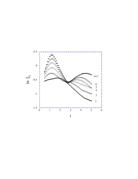
FIG. 1.: The energy correlation length $\xi_{2}$ as a function of $t$ and different layer thicknesses $n$ for $\kappa=4$ et $\gamma=1$. The size of the layers is $n=2\ldots 7$ from bottom to top.

We observe that for a very thin layer ($n=2,3$), there is only a single maximum present while two maxima develop for larger values of $n$. Comparing the location of the maxima for $n$ finite with the known values from (3) for their $n\rightarrow\infty$ limit, we see that the shift in the effective critical temperatures are quite large. Both maxima appear to show a systematic build-up normally considered typical of a thermodynamic singularity rounded by finite-size effects [3]. These observations, of one or two maxima depending on the value of $n$, large finite-size shifts of the pseudo critical temperatures and a rounding of the thermodynamic singularity, are in qualitative agreement with experiment [5, 18].

Before we can make this conclusion however, one should realize that the models usually considered in theoretical calculations and the superlattices studied experimentally are different. We shall refer to these as case A and case B, respectively. These cases differ in the way one goes from the finite system to an infinite one and it is only for the infinite system where a true phase transition can occur. Consequently, the phase diagrams for cases A and B are different. (We reemphasize that in the following discussion we refer to two-dimensional systems while experiments are carried out in three dimensions.)

1. We take a layer of $n$ spins $\frac{1}{2}$ and a layer of $n$ spins $1$. Periodic boundary conditions as explicitly written in (2) are used. The phase diagram which results when $n\rightarrow\infty$ is given in figure 2a.

2. In experiments [5, 2, 6], a procedure analogous to the following is used. One takes $n$ spins $\frac{1}{2}$ and $n$ spins $1$ and repeats this double layer $m$ times. Typically, $n$ is small and fixed but $m$ is large and formally, one should take a limit $m\rightarrow\infty$. This leads to the phase diagram in figure 2b.

FIG. 2.: Phase diagrams for the two thermodynamic limits, for two-dimensional systems. (a) Two layers with $n$ spins each, periodic boundary conditions and $n\rightarrow\infty$. (b) Superlattice of $m$ bilayers of $n$ spins of each kind and $m\rightarrow\infty$.

We first consider case A. Then, each of the two subsystems can develop long-range order by itself. Consequently, the phase diagram (figure 2a) will show four different phases. There is a paramagnetic phase where the whole system is disordered, two distinct phases where either the spin $\frac{1}{2}$ variables ($<\sigma>\neq 0$) or the spin $1$ variables ($<S>\neq 0$) are ordered while the other subsystem is disordered and a ferromagnetic phase where the system is fully ordered. The transition lines are given by eq. (3) (full line for $t_{c,\frac{1}{2}}$ and dashed line for $t_{c,1}$). In this case, the maxima observed in figure 1 should be interpreted as true thermodynamic singularities rounded by finite-size effects. Since we shall below concentrate on the properties of the order parameter close to the subsystem boundaries, we label these transitions by its surface critical properties, following the theory of surface phase transitions [19]. For the transitions from the paramagnetic phase to one of the partially ordered phases, one of the subsystems is still disordered and the order parameter of that subsystem which undergoes ordering will vanish at the boundary between the two subsystems. Along this line we have an ordinary transition. On the other hand, for the transitions from the partially ordered phases to the ferromagnetic phase one subsystem is already ordered which fixes the order parameter of the other subsystem at the subsystem boundary. Here we have an extraordinary transition. At the meeting point of the transition lines there is a special transition [20]. The scaling of the order parameter close to the subsystem boundaries is described by a different exponent than for the bulk, see Ref. [19]. These local critical exponents are in $2D$ readily calculated using conformal invariance techniques, see section 3.

For case B, corresponding to figure 2b however, the situation is different. Since each of the subsystems only contains a finite number of layers, the superlattice can only order as a whole. Thus the phase diagram contains a paramagnetic phase and a single ordered ferromagnetic phase. If $t$ is sufficiently small, a layer of $n$ spins may act as a giant spin and produce a strong thermal signal leading to a finite maximum of the specific heat or of related quantities. Since $n$ is finite, however, there is no long-range order and the magnetic moments of each layer are independent of each other. Then the specific heat as a function of temperature will show two peaks, but only the one at lower temperatures will then correspond to a (shifted and rounded) phase transition and will develop a true singularity as $m\rightarrow\infty$. Working in the framework of case B, it is misleading to call the location of the larger temperature maximum a (pseudo) critical point.

From now on we always consider case A. Then, both maxima in $\xi_{2}$ can be interpreted as signalling a transition. Also, we shall perform the subsequent scaling analyses just for the two-dimensional system, since the changes which might be needed in three dimensions are immediate and discussed in detail in the literature [3, 4].

How can one find the critical points from the finite-lattice data, when the Hamiltonians are more complicated and precise information on their location such as (3) is not available a priori ? Practically, the transition points are located using phenomenological renormalization as derived from finite-size scaling [3, 4]. Consider the quantity $R(t;n)=n/\xi(t;n)$. Then finite-size estimates for the critical point $t_{c}$ can be found by solving for $t$ the equation

$$R(t;n)=R(t;n+1)$$ (8)

if $n$ sufficiently large. A final value for $t_{c}$ is then obtained by extrapolating the resulting sequence for $n\rightarrow\infty$. Carrying out this procedure, a further subtlety is encountered as illustrated in figure 3.

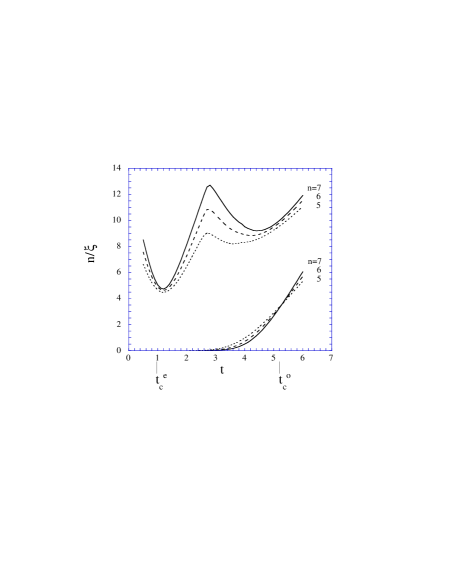
FIG. 3.: Scaled inverse correlation lengths $n/\xi_{1,2}(t)$ as a function of $t$, for $\kappa=4$ and $\gamma=1$ and several layer thicknesses $n$. The critical points are labelled $t_{c}^{o}$ and $t_{c}^{e}$ corresponding to the ordinary and extraordinary transitions. The lower (upper) curves correspond to $\xi_{1}$ ($\xi_{2}$).

Considering the finite-size scaling of the spin correlation length $\xi_{1}$ (lower curve), we see that the curves $R_{1}(t;n)$ intersect close to the critical point $t_{c}^{o}$. This is the conventional behaviour found e.g. in simple Ising models [3, 4]. For smaller values of $t$, $\xi_{1}^{-1}$ vanishes exponentially fast with $n$, which reflects the ordering of the $S=1$ subsystem in this case. Thus in order to find $t_{c}^{e}$, the second gap $\xi_{2}^{-1}$ is the natural quantity to look at and in fact represents in the partially ordered phases the lowest physical excitation, just as $\xi_{1}^{-1}$ does in the paramagnetic phase. Nevertheless, the curves $R_{2}(t;n)$ go through a minimum close to $t_{c}$ and will eventually touch each other in the $n\rightarrow\infty$ limit, but do not intersect. Although this is not in contradiction with the theory of finite-size scaling (at $t=t_{c}$, (8) is strictly valid for $n\rightarrow\infty$ only), it is remarkable that at this point the conventional finite-size techniques are no longer applicable. In order to get an estimate of $t_{c}$, one has to rely on locating a minimum of $R_{2}(t)$ or some other criterion. We stress that at $t=t_{c}^{e}$ is the only phase transition occuring in the model for case B.

This type of behaviour should be generic and although the example given does suggest that finite-size techniques may be fruitfully employed in analysing experimental data, it also shows that some care may be required. We shall see in the next section that in spite of the slightly unusual finite-size scaling, the spectrum of $H$ at all these critical points is in full agreement with the conformal invariance predictions.

To illustrate to what extent quantitative information about the critical behaviour can be extracted from our still relatively small systems ($n\leq 7$), we consider the determination of the correlation length exponent $\nu$. We look at the local maxima $t_{max}(n)$ of $\xi_{2}$ near to the point $t=t_{c}^{o}$. Finite-size scaling predicts [3, 4] that the temperature shift

$$\Delta t(n)=t_{c}^{o}-t_{max}(n)\sim n^{-1/\nu}\;\;,\;\;n\rightarrow\infty$$ (9)

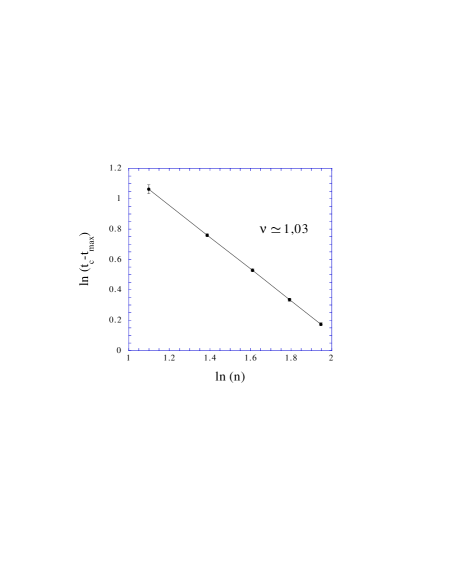
FIG. 4.: Determination of $\nu$ from the finite-size scaling of $t_{c}(n)$ near the ordinary transition for $\kappa=4$.

In figure 4, we show a log-log plot of $\Delta t(n)$ vs. $n$ and find that the asymptotic behaviour (9) is already realised for small $n$ in our toy model, although the $t_{c}(n)$ are not at all close to the $n\rightarrow\infty$ value $t_{c}^{o}$, see figure 3. From the slope in figure 4, we read off $\nu\simeq 1.03$, in good agreement with the exact result $\nu=1$. We point out that also ($3D$) data for the thermal expansion coefficient for FeF₂/ZnF₂ superlattices were successfully analysed this way [2], although also in this case $\Delta t(n)$ is large [18], leading to $\nu=0.64(4)$ in agreement with the theoretical value $\nu\simeq 0.63$ for the $3D$ Ising model.

III Critical exponents and conformal invariance

We now describe the calculation of the critical exponents. Since we work with a two-dimensional classical spin model universality class, we can use conformal invariance techniques [8, 21, 22, 23] for that purpose. Here the use of the quantum Hamiltonian rather than the classical spin model becomes advantageous, since the surface critical exponents which describe the local scaling close to the boundary between the two subsystems and in which we are mainly interested are easily obtained from the low-lying excitation spectrum of $H$. We can thus avoid the cumbersome procedure of calculating first an average $<X>$ and then subtracting from it its bulk contribution $X_{b}$ in order to get the surface term $X_{s}=<X>-X_{b}$ and then analyse its scaling behaviour. In the next two subsections, we shall first briefly collect the necessary background knowledge and shall then apply it to the problem at hand.

A Ordinary and extraordinary transitions

In two dimensions (and consequently also for quantum chains) conformal invariance specifies completely the scaling dimensions of all local observables. For a given model the first few exponents are very easily identified from the spectrum of the Hamiltonian $H$. For free or fixed boundary conditions one has [24]

$$\xi_{i}^{-1}=E_{i}-E_{0}=n^{-1}\pi x_{i}$$ (10)

where the exponents $x_{i}$ are the local critical exponents which describe scaling near the boundary between the two subsystems and the index $i$ labels the various scaling fields which occur in the model (usually, $i=1$ corresponds to the order parameter and $i=2$ to the energy density and higher gaps correspond to the scaling fields which generate correction-to-scaling terms). The scaling of the gaps (10) goes with $n$ and not with $L$ because only half of the system is critical at either the ordinary or extraordinary transitions. However, in order to be able to apply (10) to the spectrum of a quantum chain such as (2), the normalization of $H$ must be chosen such that energies and momenta are measured in the same units. One way of doing this is to recall that the surface scaling dimension of the energy density

$$x_{\epsilon,s}=2$$ (11)

which fixes the normalization $\zeta$. Furthermore, once the normalization is fixed accordingly, the conformal algebra acts as a dynamical symmetry which determines the spectrum of $H$ at criticality, viz.

$$E_{i}-E_{0}=\frac{\pi}{n}L_{0}+o(n^{-1})$$ (12)

with $L_{0}$ being one of the generators of the Virasoro algebra

$$[L_{j},L_{k}]=(j-k)L_{j+k}+\frac{c}{12}(j^{3}-j)\delta_{j+k,0}$$ (13)

The universality class is determined by the value of the central charge $c$, for the $2D$ Ising model [8, 21, 22] $c=\frac{1}{2}$.

Furthermore, the spectrum of $H$ at criticality can be found from the representations of the Virasoro algebra, see Refs. [21, 22, 8] for details. These representations are built from a highest weight state $|\Delta\rangle$ which is defined through

$$L_{0}|\Delta\rangle=\Delta|\Delta\rangle\;\;,\;\;L_{j}|\Delta\rangle=0\;\;\mbox{\rm if $j>0$}$$ (14)

and acts as the ground state for a certain representation. Excited states are generated by acting with the $L_{-j}$ ($j>0$) on $|\Delta\rangle$. Now, the principle of unitarity of the underlying field theory restricts through the Kac formula the possible values of $c$ and for each value of $c$ only permits a finite number of possible values of $\Delta$. For $c=\frac{1}{2}$, the only possible values are $\Delta=0,\frac{1}{16},\frac{1}{2}$. This leads to the three unitary irreducible representations $(0)$, $(1/16)$ and $(1/2)$ of the $c=\frac{1}{2}$ Virasoro algebra. Now, the spectrum of $H$ for the ordinary and the extraordinary transitions is given by [25, 11]

$$H^{(o)} = (0)+(1/2)\qquad\mbox{\rm ordinary}$$ (15)

$$H^{(e)} = 2(0)\qquad\qquad\quad\mbox{\rm extraordinary}$$ (16)

where the trivial prefactor $\pi/n$ is suppressed. The factor 2 for the spectrum at the extraordinary transition means that each level has the double degeneracy of the representation $(0)$. Combining these predictions with the formula (10) for the energy gaps, the critical exponents $x_{i}$ can be read off.

These predictions, which had already been checked for the spin $\frac{1}{2}$ before [25, 11], are fully reproduced in our model, in agreement with the expected universality. As an example, we take $\kappa=4$ and $\gamma=1$, but the results for the exponents do not depend on these parameters. The values for $t$ at the ordinary and extraordinary transition are from eq. (3) $t_{c}^{o}=5.30348(4)$ and $t_{c}^{e}=1$. The energy gap which is related through (10) to the exponent $x_{\epsilon,s}$ is the lowest gap in the even sector. Lattices with up to $n=7$ were used. After extrapolation [8, 26], we find $\zeta^{(o)}=2.319(6)$ and $\zeta^{(e)}=0.996(5)$ for the ordinary and the extraordinary transitions, respectively [27]. In table I, we give the extrapolated estimates for the first four rescaled gaps $x_{i}=(E_{i}-E_{0})n/(\zeta\pi)$ for the ordinary and extraordinary transitions together with the predictions following from conformal invariance. For the extraordinary transition, all levels were found to be doubly degenerate in the $n\rightarrow\infty$ limit but with an exponentially small splitting between pairs of levels for $n$ finite. As should be expected from the algebraic construction of the spectrum of $H$, the differences between values of the $x_{i}$ which belong to the same representation are integers. This reconfirms our determination of $\zeta$. For the ordinary transition, we see that $x_{\epsilon,s}=x_{3}=2$ and $x_{1}=x_{\sigma,s}=\beta_{1}/\nu=1/2$ is the surface magnetization exponent, where $\beta_{1}$ describes the scaling of the order parameter at the surface, $m_{1}\sim(T_{c}-T)^{\beta_{1}}$ and $\nu$ is the bulk correlation length exponent [19].

For the extraordinary transition, a little care is necessary in identifying the surface exponents. The order parameter is odd under spin reversal and the most local of all scaling operators. When this operator acts on the ground state, it creates the state with the lowest gap in the spectrum. Thus in our model $x_{\sigma,s}^{(1)}=x_{0}=0$. On the other hand, in the literature (e.g. Ref. [19] and refs. therein), the extraordinary transition is defined with respect to those degrees of freedom which become critical in the presence of a boundary which is already ordered. To read off the corresponding exponents, one should discard the double degeneracy of the spectrum, which is merely due to the ordering of the other subsystem. We then have $x_{\epsilon,s}=x_{\sigma,s}^{(2)}=x_{1}=2$. This is in agreement with the expected scaling relation [28, 19] $x_{\sigma,s}=\beta_{1}^{ex}/\nu=2-\alpha=2$.

B Special transition

At the special transition, both subsystems become critical simultaneously. In addition, the Ising quantum chain has the peculiarity that the boundary coupling $\gamma$ is marginal. The critical behaviour of the model can be described using previous results for the scaling behaviour of an Ising model with (semi-)infinite defect lines, which has been extensively studied for a long time [10, 11, 12, 29, 30, 31, 32, 33], see Ref. [23] for a review. The local critical exponents depend continuously on the coupling $\gamma$. The mapping of coupled Ising layers to a $2D$ Ising model with a star-like configuration of semi-infinite defect lines was exactly derived for coupled spin $\frac{1}{2}$ Ising models [10, 11, 12]. The surface critical exponents can be read off the energy spectrum [30]

$$\xi_{i}^{-1}=E_{i}-E_{0}=L^{-1}2\pi x_{i}(\gamma)$$ (17)

provided that the normalization $\zeta$ is fixed such that conformal invariance is applicable. We find $\zeta$ from the requirement $x_{\epsilon,s}=1$, which is also a necessary condition for the marginality of the coupling $\gamma$.

The conformal theory is in this case more complicated than for the ordinary or extraordinary transitions. For the spin $\frac{1}{2}$ Ising model, one can construct the Hamiltonian spectrum either through non-unitary Virasoro generators [31], Kac-Moody algebras [34] or alternatively rely on boundary conformal field theory [33]. Here we shall restrict ourselves to a simple way to characterize the spectrum.

Taking the spin $\frac{1}{2}$ case as a guide, we expect that for $n$ large, the low-lying excitation spectrum of $H$ can be recovered from the free fermion Hamiltonian [31, 32]

$$H = \frac{2\pi}{L}\sum_{r=0}^{\infty}\left[\left(r+\frac{1}{2}-\Delta\right)n_{r}^{(-)}+\left(r+\frac{1}{2}+\Delta\right)n_{r}^{(+)}\right]$$ (18)

$$- \frac{\pi}{6L}\left(\frac{1}{2}-6\Delta^{2}\right)$$ (19)

where $n_{r}^{(\pm)}$ are fermionic number operators and $\Delta$ depends on $\gamma$. Non-universal terms which do not enter into the gaps are already subtracted. In general, for states in the even sector (with an even number of occupied fermionic states) and in the odd sector, there will be different values $\Delta_{0}(\gamma)$ and $\Delta_{1}(\gamma)$, respectively. Now the lowest levels of $H$ can be easily written down in terms of $\Delta_{0,1}$. For example, the lowest exponents in the odd sector are

$$x_{\sigma,s} = \frac{1}{2}(\Delta_{1}-1)^{2}-\frac{1}{2}\Delta_{0}^{2}$$ (20)

$$x_{\sigma^{\prime},s} = \frac{1}{2}(\Delta_{1}+1)^{2}-\frac{1}{2}\Delta_{0}^{2}$$ (21)

and the lowest exponents in the even sector are

$$x_{\epsilon,s} = 1$$ (22)

$$x_{\epsilon^{\prime},s} = 2-2\Delta_{0}$$ (23)

$$x_{\epsilon^{\prime\prime},s} = 2+2\Delta_{0}$$ (24)

All these exponents correspond to conformal highest weight states. In addition, conformal invariance implies that if the exponent $x_{i}$ of a highest weight state occurs in the spectrum, also $x_{i}+k$ with $k=1,2,3\ldots$ is present, with a known degeneracy which only depends on $k$ (and which is 1 for the lowest two levels). From equations (21,23), the values of $\Delta_{0,1}$ for a given $\gamma$ are found. While these are known exactly for the spin $\frac{1}{2}$ case [32, 10, 11, 12], these have be determined numerically for the case at hand.

We first fix the normalization constant $\zeta$ from the condition $x_{\epsilon,s}=1$. This condition means that the scaled lowest gap $A_{even}=n\Delta E_{even}=\frac{1}{2}L\Delta E_{even}$ in the even sector should be equal to $\pi\zeta$, see (17). In table II, we give $A_{even}$ for several values of $\gamma$. We find that within our numerical accuracy, its value is independent of $\gamma$ (the apparent deviation seen for $\gamma=0.5$ is an artifact from the extrapolation of our short sequences and should disappear if larger lattices could be taken into account) and conclude that the normalization $\zeta$ is independent of $\gamma$. That is only to be expected from earlier results for spin $\frac{1}{2}$ Ising models with defect lines [32, 10, 11]. The final value of $\zeta$ is taken from the values of $\gamma=0.75\ldots$ and $\gamma=0.87\ldots$ where convergence is best and we obtain $\zeta=0.5964(2)$.

The numerical estimation for the higher gaps is made difficult by (a) the relatively short sequences available ($n\leq 7$) and (b) the fact that for $n$ finite, level crossings between different sequences occur. In table III we give the extrapolated results for the critical exponents $x_{i}=L/(2\pi\zeta)(E_{i}-E_{0})$ for several values of $\gamma$. When no information is given, our sequences did not converge reliably. We now want to compare these with the spectrum following from (19). First, we use (21,23) to determine $\Delta_{0,1}$, which are also given in table III. Depending on the value of $\gamma$, it turned out to be numerically preferable to fix first $\Delta_{0}$ from (23) and than use this value and the estimate of $x_{\sigma}$ to find $\Delta_{1}$ or alternatively determine $\Delta_{1}$ from the difference $x_{\sigma^{\prime},s}-x_{\sigma,s}$, which is independent of $\Delta_{0}$. The values of $\Delta_{0,1}$ were then used to calculate the other exponents which are listed in table III as ‘expected’. When no error is given in these columns, the expected value is exact.

We see that in general the extrapolated estimates for the higher gaps agree with the conformal invariance prediction to within a few per cent. A particular problem arises for $\gamma=0.5$, where the converge for $x_{\epsilon}$ is particularly slow. In that case, we are not able to sensibly to specify accuracies for $\Delta_{0,1}$ and the correspondence between the ‘numerical’ and the ‘expected’ data is more qualitative. The situation here could only be improved by going to larger lattices. On the other hand, for the other values of $\gamma$, we obtain a nice agreement between the ‘numerical’ data and the ‘expected’ free fermion spectrum. We point out that the beginning of several conformal towers (that is, with $x_{i}$ also $x_{i}+1$ and even $x_{i}+2$ are found in the spectrum) is observed. The fact that this level spacing comes out correctly is a further confirmation of our determination of the normalization constant $\zeta$. On the other hand, we have not been able to go sufficiently high in the spectrum to check the degeneracies of the excited states.

We see that the scaling behaviour of our model is described in terms of a free fermion system. This should be expected on the basis of universality, although this free fermion description of a spin $1$ model is not at all obvious from the lattice formulation. Nevertheless, there is an important distinction with respect to the spin $\frac{1}{2}$ case. Recall that the value of $\gamma$ is the same at both subsystem boundaries. Had we coupled two spin $\frac{1}{2}$ systems, we would have found [32, 10, 11] $\Delta_{0}=0$, which is not the case in our model, see table III.

IV Order parameter profiles

So far, we have calculated the critical exponents which describe the scaling of observables close to the subsystem boundary. We now ask for the form of the order parameter profiles close to that interface.

A Generalities

The calculation of the order parameter on a finite lattice poses a conceptual problem. The natural candidate, $<M>=\langle 0|M|0\rangle=0$ on any finite lattice. This difficulty can be overcome by first introducing a small magnetic field $h$, calculating $<M>$ in the presence of $h$, take the infinite system limit $L\rightarrow\infty$ and only then let $h\rightarrow 0$. In practice, rather than performing numerically this double limit, the following trick which goes back to Yang is used. In the ordered phase(s), the ground state is already on a finite lattice almost degenerate, where the energy splitting decreases exponentially with $L$. Introducing an infinitesimal magnetic field $h$ into $H$ and working within degenerate first-order perturbation theory in $h$, the order parameter on the site $i$ is given by [35]

$$m(i)=\langle 1|M(i)|0\rangle$$ (25)

where $|0\rangle$ and $|1\rangle$ are the lowest eigenstates in the even and odd sectors, respectively. For our model (2), the magnetization operator $M(i)$ is

$$M(i)=\left\{\begin{array}[]{cc}\sigma^{z}_{i}&\mbox{\rm; spin $\frac{1}{2}$ region}\\ S^{z}_{i}&\mbox{\rm; spin $1$ region}\end{array}\right.$$ (26)

so that $M(i)$ is normalized such that $|M(i)|\leq 1$ for all sites. It is well known [36] that the finite-lattice order parameter calculated from (25) has the correct scaling behaviour. The dependence of the order parameter profiles on $S$ deep in the ordered phase has also been studied [37].

Practically, for the computation of the eigenvectors $|0\rangle,|1\rangle$, it is not necessary to store all the intermediate Lánczos vectors. This can be avoided by running the Lánczos algorithm twice, where the first pass furnishes the weights by which the intermediate vectors contribute to $|0\rangle,|1\rangle$ and in the second pass the eigenvectors themselves can be accumulated [15].

B Ordinary and extraordinary transitions

Before presenting our results for the order parameter profiles at the various transitions, let us adapt the predictions from finite-size scaling theory [3, 4, 36] to the situation at hand. We are interested in the local order parameter $m(i)$ rather than the full magnetization $m=\sum_{i}m(i)$. One should distinguish whether $m(i)$ is measured far away or close to the subsystem boundary. In the first case, when the site $i$ is well in the bulk, we expect

$$m(i)=n^{-x_{\sigma}}{\cal M}\left(\frac{2i-1}{4n}\right)$$ (27)

In the second case, when $i$ is close to the boundary, we should have[38]

$$m(i)=a^{-x_{\sigma}}\left(\frac{n}{a}\right)^{-x_{\sigma,s}}\widetilde{\cal M}\left(\frac{i-n-1/2}{a}\right)$$ (28)

Here, $x_{\sigma}$ and $x_{\sigma,s}$ are the bulk and surface critical exponents calculated in the previous section, $\cal M$ and $\widetilde{\cal M}$ are scaling functions, $i=1,2,\ldots,2n$ is measured from the left boundary of the $S=1$ subsystem, $n$ is the layer thickness and $a$ the lattice constant. We point out that the arguments of the two scaling functions are different.[38] In the first case, the scaling is such that the total system size is kept fixed and the lattice constant $a\rightarrow 0$, while in the second case, $a$ is kept fixed and the system size $L=2n\rightarrow\infty$.

These predictions are confirmed by our numerical results. Consider first the ordinary transition. Again, we take $\kappa=4$ and $\gamma=1$ as an example. In figure 5, we rescale our magnetization profiles according to (27) with $x_{\sigma}=1/8$ and we see that indeed for the portion of the lattice which is far enough for the subsystem boundaries, a data collapse occurs even for the small lattices considered here. Also, we see that in the immediate vicinity of the subsystem boundaries, the scaling description (27) no longer applies. Similar plots for the bulk scaling can be obtained for the other transitions but will not be presented here, but see figure 9 below.

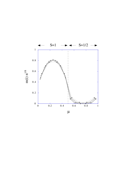
FIG. 5.: Order parameter for the ordinary transition, scaled with the bulk exponent $x_{\sigma}=1/8$ for $\kappa=4$ and $\gamma=1$ as a function of $\mu=(2i-1)/4n$. The regions of spin $S=1$ and $S=\frac{1}{2}$ are indicated and the boundary between them is shown by the dotted line. The symbols correspond to $n=4$ (diamonds), $n=5$ (triangles), $n=6$ (squares) and $n=7$ (circles).

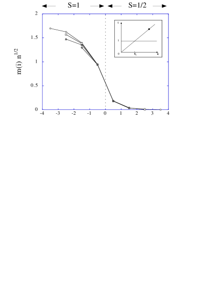
FIG. 6.: Scaled profile of the order parameter for the ordinary transition, for $\kappa=4$ and $\gamma=1$ as a function of $\widetilde{\mu}=i-n-\frac{1}{2}$. The inset shows the location of the transition point in the phase diagram. The correspondence of the symbols to the layer thickness $n$ is the same as in figure 5.

In figure 6, we display the local scaling of the order parameter close to one of the subsystem boundaries according to (28). For the ordinary transition, $x_{\sigma,s}=1/2$ and we set $a=1$. We see that in the first two monolayers around both sides of the interface, the data collapse onto the scaling form (28). However, going beyond the first two monolayers, it is apparent that there is a crossover towards the bulk scaling form (27). It is apparent that the surface scaling only occurs in a very thin layer close to the boundary. We remark that this is consistent with experimental observations that thin magnetic layers on a non-magnetic substrate show two-dimensional critical behaviour for layer thicknesses of less than about two monolayers and cross over to three-dimensional criticality for only slightly thicker layers [39].

A similar behaviour is also found for the extraordinary transition. However, as already mentioned in discussing the spectra, it is sensible to distinguish two ‘order parameters’. These are

$$m^{(1)}(i) = \langle 1|M(i)|0\rangle$$ (29)

$$m^{(2)}(i) = \langle 1|M(i)|0^{\prime}\rangle\simeq\langle 1^{\prime}|M(i)|0\rangle$$ (30)

where $|0^{\prime}\rangle$ and $|1^{\prime}\rangle$ are the first excited states in the even and odd sectors and the approximate equality between the two forms for $m^{(2)}$ holds up to terms exponentially small in $L$. Note that here the ordering at the subsystem boundary is provided through the subsystem already in its ordered phase for $n\rightarrow\infty$ and not through fixing the spins at the boundary. The profile for $m^{(1)}$, where the surface exponent $x_{\sigma,s}^{(1)}=0$, is shown in figure 7. Again, we see that for the $S=\frac{1}{2}$ subsystem, we have a data collapse according to (28) for the first two monolayers next to the boundary and for larger values of $i$, the is a rapid crossover toward the bulk scaling (27). Since the $S=1$ subsystem is ordered, finite-size effects are exponentially small there.

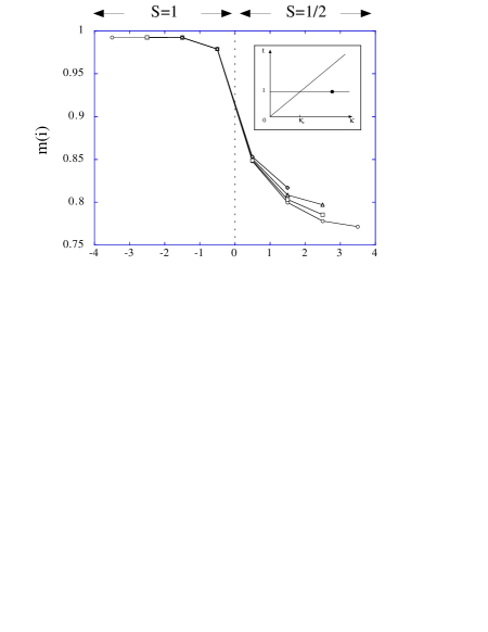
FIG. 7.: Profile for the order parameter $m^{(1)}$ at the extraordinary transition for $\kappa=4$ and $\gamma=1$ as a function of $\widetilde{\mu}$. The inset shows the location of the transition point in the phase diagram. The correspondence of the symbols to the layer thickness $n$ is the same as in figure 5.

C Special transition

This case is of particular interest, since the exponent $x_{\sigma,s}$ does depend on $\gamma$. It is therefore interesting to ask whether the profiles are affected by changing $\gamma$ as well. The bulk scaling behaviour (27) with $x_{\sigma}=1/8$ is recovered as in the other transitions.

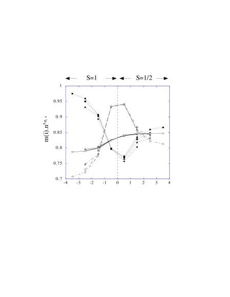
FIG. 8.: Scaled profiles for the order parameter at the special transition for several values of $\gamma$ as a function of $\widetilde{\mu}$. The dotted curves with full symbols correspond to $\gamma=\frac{1}{2}$, the full curves with open symbols to $\gamma=0.877111$ and the dash-dotted curves with open symbols corresponds to $\gamma=2$. The correspondence of the symbols to the layer thickness $n$ is the same as in figure 5.

In figure 8, we show for three values of $\gamma$ the local scaling of the order parameter, where the values of $x_{\sigma,s}$ are taken from table III. On both sides of the boundary, we find a data collapse according to (28) for the first few boundary layers and for larger values of $i$, a crossover towards the bulk scaling (27). In addition, we see that the form of the scaling function $\widetilde{\cal M}$ does depend on $\gamma$. For $\gamma\simeq 0.87$, we have $x_{\sigma,s}\simeq x_{\sigma}=1/8$ (see table III) and the distinction between local and bulk scaling is somewhat washed out.

Concerning the shape of the scaling function $\widetilde{\cal M}(\widetilde{\mu})$, we see that for the special transition, it can be a non-monotonous function of $\widetilde{\mu}$. For the ordinary and the extraordinary transitions, however, it is a monotonous function of $\widetilde{\mu}$ and this holds independently of the value of $\gamma$. For the special transition, $\widetilde{\cal M}(\widetilde{\mu})$ is only monotonous if $\gamma\simeq\kappa_{c}$. Qualitatively, this can be explained as follows.

First, if $\gamma\simeq\kappa_{c}$, the boundary coupling takes the effective mean value which smoothly interpolates between the two different regimes. Since both systems become critical simultaneously at the special transition, the scaling functions simply interpolates smoothly between the values of the magnetization finite-size scaling amplitudes in the two subsystems. Since these amplitudes are different, even for $x_{\sigma,s}(\gamma)=1/8$, the scaling function $\widetilde{\cal M}(\widetilde{\mu})$ will not become a constant. Second, consider $\gamma>\kappa_{c}$. Then the spins on both sides of the boundary are more strongly coupled together than two spins in either subsystem. Since the $S=0$ state in the spin $1$ subsystem does not contribute to the energy, this leads to an enhancement of states where the boundary spins on both sides are up. Indeed, we checked that already for $\gamma=4$, the local order parameter on both sides of the boundary is close to saturation. Thus, we have a large value of $m(i)$ close to the boundary which then falls back to an average value for each of the subsystem, in agreement with figure 8. Finally, for $\gamma<\kappa_{c}$, the spins on both sides of the boundary are more weakly coupled than average spins. This favors states with a smaller value of $m(i)$ close to the subsystem boundary.

On the other hand, for the ordinary or the extraordinary transition, one subsystem is much more ordered than the other one. If $\gamma$ is large, the first spin across the boundary is strongly aligned with the spins of the more ordered subsystem and if $\gamma$ is small, the coupling of the first spin to the more ordered subsystem is reduced. This leads to an effective translation of the order parameter profile without affecting its form.

D Magnetization profiles and conformal invariance

In $2D$, conformal invariance states that the profile of a local scaling operator $\varphi$ with bulk scaling dimension $x_{\varphi}$ is on an infinitely long strip of finite width $L$ and with the same type of boundary conditions on both sides (and in particular for free boundary conditions) given by [40]

$$\langle\varphi(v)\rangle={\cal A}_{\varphi}\left(\frac{L}{\pi}\sin\left(\frac{\pi v}{L}\right)\right)^{-x_{\varphi}}\sim v^{-x_{\varphi}}\;\;,\;\;v\rightarrow 0$$ (31)

where $v$ measures the position across the strip and ${\cal A}_{\varphi}$ is a non-universal constant. The scaling function for mixed boundary conditions is also known for minimal conformal theories [41]. This result only depends on the transformation properties of the scaling operator $\varphi$. Furthermore, this result carries over to the profiles on quantum chains.

When we try to apply this to the order parameter at the ordinary transition, we should find ${\cal A}_{\sigma}=0$ due to symmetry. However, the finite-lattice estimates for $m(i)$ obtained from eq. (25) above involved an infinitesimal magnetic field $h$, which (a) invalidates the above symmetry argument and (b) leads to a new effective exponent $x_{\varphi}=x_{\sigma}-x_{\sigma,s}$. This is seen as follows. From our numerical data, we have found the scaling form (27)

$$m_{L}(z)=L^{-x_{\sigma}}{\cal M}(\mu)\;\;,\;\;\mu=z/L$$ (32)

On the other hand, close to the boundary, the order parameter should show surface finite-size scaling $m_{L}\sim L^{-x_{\sigma,s}}$. This implies for the scaling function, e.g. Ref. [19]

$${\cal M}(\mu)\sim\mu^{x_{\sigma,s}-x_{\sigma}}\;\;,\;\;\mu\rightarrow 0$$ (33)

from which $x_{\varphi}$ can be identified. Eq. (33) was also confirmed within the framework of the $\epsilon$ expansion[42] and for the Ising quantum chain with an aperiodic modulation generated by the Fredholm sequence.[43] For the $2D$ Ising model, we remark that also in the presence of a small surface magnetic field [44] $h_{1}$ the spatial dependence of the magnetization near to the surface scales as $z^{3/8}$, which is the same as obtained from eq. (33).

We now try to extend (33), derived for small values of $\mu$ only, to larger values of $\mu$. If we accept[45] that the estimate eq. 25) for the spontaneous magnetization transforms covariantly under conformal transformations, we can combine eqs. (31,33). Then the exact finite-size scaling function at the ordinary transition would be[45]

$${\cal M}(\mu)=A_{\sigma}\left(\sin 2\pi\mu\right)^{x_{\sigma,s}-x_{\sigma}}$$ (34)

taking into account that for our model, only the section $0\leq\mu\leq\frac{1}{2}$ is actually critical at the ordinary transition for $\kappa>\kappa_{c}$.

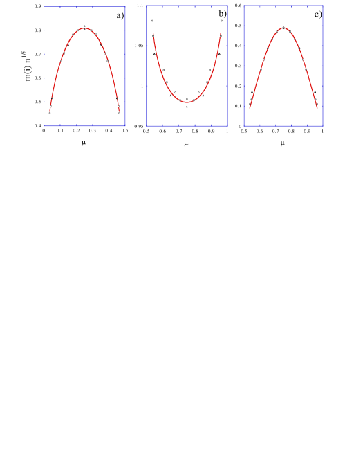
FIG. 9.: Comparison of the conformal invariance prediction for the scaled order parameter profiles $m(i)n^{1/8}$. Only the part of the system which is critical is shown. The graphs give for (a) the ordinary transition, (b) the extraordinary transition with $m^{(1)}$ and (c) for $m^{(2)}$ at $\kappa=4$ and $\gamma=1$. The correspondence of the symbols to the layer thickness $n$ is the same as in figure 5.

In figure 9a, we compare (34) to the numerical data. First, we observe a data collapse from several system sizes onto a single curve. Second, the form of the scaling function agrees nicely with eq. (34). The same result has also been found for the Hilhorst-van Leeuven model [45, 43]. Since for the $2D$ Ising model, (33) remains unchanged even in the presence of a small surface magnetic field,[44] $\cal M$ should be independent of a small $h_{1}$ for the ordinary transition.

Let us compare the finite-size scaling functions for the profiles coming from (31) and (34). The first one is based on a continuum description of the profile in the half-infinite system which is then conformally transformed onto the strip [40]. Very close to the boundary, a continuum description may no longer be applicable. Indeed, for unitary conformal theories such as the Ising model, the critical exponents $x_{\varphi}>0$ and the profile as it stands will diverge at the boundary, in disagreement with existing numerical data. On the other hand, the second form is constructed to be consistent with both bulk finite-size scaling deep inside the system and surface finite-size scaling close to the boundary. In order to match this with the functional form required from conformal invariance, it is necessary to assume that the exponent $x_{\sigma}-x_{\sigma,s}$ governs the scaling of the matrix element (25) (calculated in an infinitesimal magnetic field which breaks global symmetry) used to estimate the finite-size order parameter, rather than the conventional order parameter scaling dimension $x_{\sigma}>0$. While this approach certainly is in agreement with the numerical data for the whole strip, it is not yet understood how the above dimensional transmutation can be explained.

In addition, we find that the same functional form also describes the order parameter profiles for the extraordinary transition, as shown in figure 9. The numerical data are again consistent with scaling (note that the overall scale in figure 9b is abount an order of magnitude larger than in the other two cases). Specifically, we find from a fit

$${\cal M}(\mu)=\left\{\begin{array}[]{lll}A_{\sigma}(\sin 2\pi\mu)^{3/8}&,\;A_{\sigma}\;\;\simeq 0.80&\mbox{\rm ord.}\\ A_{\sigma}^{(1)}(\sin 2\pi\mu)^{-1/16}&,\;A_{\sigma}^{(1)}\simeq 0.98&\mbox{\rm ex., $m^{(1)}$}\\ A_{\sigma}^{(2)}(\sin 2\pi\mu)^{9/8}&,\;A_{\sigma}^{(2)}\simeq 0.49&\mbox{\rm ex., $m^{(2)}$}\end{array}\right.$$ (35)

Tentatively, the profile for $m^{(1)}$ (which is not given by (31) because the ‘ordered’ subsystem is still finite, see eq. (30)) can be explained as follows. This order parameter is sensible to the ordering which occurs at the ordinary transition. At the extraordinary transition, these degrees of freedom have become massive and thus have a short effective correlation length $\xi_{eff}$. Then the fluctuating spins would see a fixed boundary on one side but because $\xi_{eff}\ll L$ the other boundary should appear as open. However, for mixed boundary conditions, it is known that [25, 8] $x_{\sigma,s}=\frac{1}{16}$. Then $-x_{\varphi}=\frac{1}{16}-\frac{1}{8}=-\frac{1}{16}$ in agreement with the numerical data.

Finally, the above argument does not reproduce the profiles for the special transition. This is due to the fact that the two-point correlation functions are more complicated [33] than the simple power-law form which underlies the derivation [40] of (31).

V Summary

We have studied the transitions arising in a pair of magnetic layers, coupled through short-ranged interactions and described by Ising models. This study was motivated by ongoing experiments on similar systems. We have found the variation of the ‘specific heat’ with the temperature and studied the scaling of the order parameter profiles at the phase transition points. Our aim was to check out a scaling analysis which should also be applicable to experimental data in $3D$.

We have reemphasized that the systems usually studied in experiments and the models best suited for theoretical analysis are not completely identical and care is needed in the comparison of the two, as exemplified in the two phase diagrams in figure 2.

To simplify the theoretical analysis, we used a two-dimensional model of layers of spin chains, although the experiments [5, 39, 6] involve two-dimensional layers stacked in the third dimension. This was for us no serious disadvantage, since the scaling arguments used here can be extended to three dimensions in a well-known way [2, 3, 4]. In addition, conformal invariance techniques could be used to simplify the calculation of the surface critical exponents we were interested in. This calculation reconfirmed the expected universality of the surface critical exponents found for the ordinary, extraordinary and special transition (where in the $2D$ Ising model, the surface coupling is marginal).

Our results on how the ‘specific heat’ depends on the layer thickness $n$ are qualitatively the same as seen experimentally [5]. Our results also suggest that if the layer thickness can be precisely controlled, one might get a trade-off in no longer having to achieve a very fine temperature control and still being able to measure fluctuation-dominated critical exponents to good accuracy.

Our study for the order parameter profiles was motivated by the existing experimental techniques to measure the magnetic moments of a single monolayer [6]. While for an infinite system, the critical point magnetization vanishes, for finite lattices a non-trivial finite-size scaling behaviour of the order parameter profiles is obtained. We found two types of finite-size scaling at the transitions. Far away from the subsystem boundaries, we get a bulk finite-size scaling (27) governed by the bulk exponent $x_{\sigma}=\beta/\nu=1/8$. In the immediate vicinity (and on both sides) of the boundary, however, the order parameter finite-size scaling (28) is governed by the surface critical exponent $x_{\sigma,s}=\beta_{1}/\nu$ whose value depends on the type of the surface transition.

For the ordinary and the extraordinary transitions, the data for finite-size scaling of the order parameter profile scaling function $\cal M$ (measured in an infinitesimal magnetic field) suggest in $2D$ an exact scaling function from consistency with bulk and surface finite-size scaling and with conformal invariance. It remains a challenge to derive a similar result for the special transition. It is not yet clear how to address the problem of calculating the surface scaling function $\widetilde{\cal M}$. In any case, a continuum approach, which underlies the conformal invariance arguments used for the determination of $\cal M$, does not seem to be feasible in that case.  
 
It is a pleasure to thank R. Camley, F. Iglói and L. Turban for useful discussions.

	ordinary			extraordinary
$i$	numerical	expected		numerical	expected
0	0	0		0	0
1	0.4994(6)	$1/2$		2	2
2	1.496(7)	$3/2$		3.01(2)	3
3	2	2		3.95(6)	4
4	2.505(9)	$5/2$		4.9(2)	5

TABLE I.: Conformal spectrum of the surface exponents $x_{i}$ for the ordinary and extraordinary transitions at $\kappa=4$ and $\gamma=1$. The numbers in brackets give the estimated uncertainty in the last given digit.

$\gamma$	0.5	0.65	0.754222	0.877111	1
$A_{even}$	1.945(3)	1.889(7)	1.8731(8)	1.8745(5)	1.88(2)

TABLE II.: Scaled and extrapolated lowest gap $A_{even}=\pi\zeta$ in the even sector at the special transition for several values of $\gamma$. The numbers in brackets give the estimated extrapolation error in the last digit.

	$\gamma=0.5$		$\gamma=0.754222$		$\gamma=0.877111$		$\gamma=1$
$i$	numerical	expected	numerical	expected	numerical	expected	numerical	expected
1	0.231(1)	0.20	0.1436(6)	0.144(2)	0.1103(7)	0.1103(5)	0.0841(5)	0.084(5)
2	0.971(3)	0.91	0.999(1)	1	1.000(1)	1	1.00(2)	1
3	1.034(5)	1	1.10(3)	1.072(4)	1.113(6)	1.1103(5)	1.11(2)	1.084(5)
4	1.095(3)	1.20	1.12(2)	1.144(2)	1.168(5)	1.168(2)	1.232(5)	1.232(5)
5	1.72(3)	1.70	1.94(1)	1.94(1)	1.92(1)	1.92(1)	1.9(1)	1.78(4)
6	1.92(3)	1.91	1.995(5)	2	2.00(2)	2	2.0(1)	2
7	1.99(2)	2	2.03(3)	2.06(1)	2.11(1)	2.08(1)	2.1(1)	2.084(5)
8	-	2.20	2.11	2.072(4)	-	2.1103(5)	2.18(3)	2.22(4)
9	-	2.30	2.145(8)	2.144(2)	-	2.168(2)	-	2.232(5)
$\Delta_{0}$	0.15		0.030(5)		0.040(5)		0.11(3)
$\Delta_{1}$	0.36		0.464(2)		0.529(1)		0.574(4)

TABLE III.: Conformal spectrum of the scaling dimensions $x_{i}(\gamma)$ at the special point $t=1,\kappa=0.754222$. The values of $\Delta_{0,1}$ used in comparing with the free fermion Hamiltonian (19) are also given. The numbers in brackets give the estimated uncertainty in the last given digit.

REFERENCES

- [1] Unité de recherche associée au CRNS no. 155
- [2] D. Lederman, C.A. Ramos, V. Jaccarino and J.L. Cardy, Phys. Rev. B48, 8365 (1993).
- [3] M.N. Barber in Domb and Lebowitz (Eds) Phase Transitions and Critical Phenomena, Vol. 8, ch. 2, Academic Press (New York 1983).
- [4] V. Privman (Ed) Finite Size Scaling and Numerical Simulation of Statistical Systems, World Scientific (Singapore 1990).
- [5] D. Lederman, C.A. Ramos and V. Jaccarino, J. Phys. Cond. Matt. 5, A373 (1993).
- [6] Ph. Bauer, S. Andrieu and M. Piecuch, Nouv. Cim. 18D, 299 (1996); Ph. Bauer, S. Andrieu, M. Lemine and M. Piecuch, E-MRS Conference, Straßburg June 1996, to appear in J. Mag. Mag. Mat.
- [7] M. Suzuki, Prog. Theor. Phys. 46, 1337 (1971); E. Fradkin and L. Susskind, Phys. Rev. D17, 2637 (1978).
- [8] P. Christe and M. Henkel, Introduction to Conformal Invariance and its Applications to Critical Phenomena, Springer (Berlin 1993).
- [9] D. Bitko, T.F. Rosenbaum and G. Aeppli, Phys. Rev. Lett. 77, 940 (1996).
- [10] H. Hinrichsen, Nucl. Phys. B336, 377 (1990).
- [11] B. Berche and L. Turban, J. Phys. A24, 245 (1991).
- [12] D-G. Zhang, B.-Z. Li and M.-G. Zhao, Phys. Rev. B53, 8161 (1996).
- [13] P. Pfeuty, Ann. of Phys. 57, 79 (1970).
- [14] W. Hofstetter and M. Henkel, J. Phys. A29, 1359 (1996).
- [15] E. Dagotto, Rev. Mod. Phys. 66, 763 (1994).
- [16] If and has a logarithmic singularity as happens for the Ising model, a similar analysis shows that .
- [17] In the simple spin systems usually considered this distinction is not necessary and and are propotional to each other.
- [18] C.A. Ramos, D. Lederman, A.R. King and V. Jaccarino, Phys. Rev. Lett. 65, 2913 (1990).
- [19] H.W. Diehl in Domb and Lebowitz (Eds) Phase Transitions and Critical Phenomena, Vol. 10, ch. 2, Academic Press (New York 1986).
- [20] Since the model eq. (2) is two-dimensional, the layers cannot order for finite and thus there is no surface transition. This would be different in a three-dimensional model, where surface transitions may occur [19].
- [21] J.L. Cardy, in Domb and Lebowitz (Eds) Phase Transitions and Critical Phenomena, Vol. 11, ch. 2, Academic Press (New York 1987).
- [22] C. Itzykson and J.-M. Drouffe, Statistical Field Theory, Vol. 2, ch. 9, Cambridge University Press (Cambridge 1989).
- [23] F. Iglói, I. Peschel and L. Turban, Adv. Phys. 42, 683 (1993).
- [24] J.L. Cardy, J. Phys. A17, L385 (1984).
- [25] T.W. Burkhardt and I. Guim, Phys. Rev. B35, 1799 (1987); J.L. Cardy, Nucl. Phys. B275, 200 (1986); G.v. Gehlen and V. Rittenberg, J. Phys. A19, L631 (1986).
- [26] M. Henkel and G. Schütz, J. Phys. A21, 2617 (1988).
- [27] These values for are close to the ones found for the spin and spin Ising model separately [14], thereby confirming that only the critical degrees of freedom make a contribution to .
- [28] A.J. Bray and M.A. Moore, J. Phys. A10, 1927 (1977).
- [29] R.V. Bariev, Sov. Phys. JETP 50, 613 (1979); B.M. McCoy and J.H.H. Perk, Phys. Rev. Lett. 44, 840 (1980); L.P. Kadanoff, Phys. Rev. B24, 5382 (1981); D.B. Abraham, L.F. Ko and N.M. Švrakic, J. Stat. Phys. 56, 563 (1989).
- [30] L. Turban, J. Phys. A18, L325 (1985).
- [31] M. Henkel and A. Patkós, Nucl. Phys. B285, 29 (1987).
- [32] M. Henkel, A. Patkós and M. Schlottmann, Nucl. Phys. B314, 609 (1989).
- [33] G. Delfino, G. Mussardo and P. Simonetti, Nucl. Phys. B432, 518 (1994); M. Oshikawa and I. Affleck, Vancouver preprint, hep-th/9606177.
- [34] M. Baake, P.Chaselon and M. Schlottmann, Nucl. Phys. B314, 625 (1989).
- [35] C.N. Yang, Phys. Rev. 85, 808 (1952).
- [36] K. Uzelac and R. Jullien, J. Phys. A14, L151 (1981); C.J. Hamer, J. Phys. A15, L675 (1982).
- [37] H.J. Mikeska, S. Miyashita and G.H. Ristow, J. Phys. Cond. Matt. 3, 2985 (1991); M. Henkel, A.B. Harris and M. Cieplak, Phys. Rev. B52, 4371 (1995).
- [38] These forms can be obtained from where is the distance across the strip. Eq. (27) is recovered in the limit . Eq. (28) is obtained in the limit with fixed and .
- [39] M. Farle and K. Baberschke, Phys. Rev. Lett. 58, 511 (1987); W. Dürr, D. Kerkmann and D. Pescia, Int. J. Mod. Phys. B4, 401 (1990); Z.Q. Qiu, J. Pearson and S.D. Bader, Phys. Rev. Lett. 67, 1646 (1991); C. Rau and C. Jin, J. Physique Colloque C8, 49, C8-1627 (1988).
- [40] T.W. Burkhardt and E. Eisenriegler, J. Phys. A18, L83 (1985).
- [41] T.W. Burkhardt and T. Xue, Nucl. Phys. B354, 653 (1991).
- [42] G. Gompper, Z. Phys. B56, 217 (1984).
- [43] D. Karevski, thèse de doctorat, Nancy 1996.
- [44] U. Ritschel and P. Czerner, Essen preprint, cond-mat/9603011.
- [45] F. Iglói and L. Turban, to be published.