Electron Dynamics in Intentionally Disordered Semiconductor Superlattices

Abstract

We study the dynamical behavior of disordered quantum-well-based semiconductor superlattices where the disorder is intentional and short-range correlated. We show that, whereas the transmission time of a particle grows exponentially with the number of wells in an usual disordered superlattice for any value of the incident particle energy, for specific values of the incident energy this time increases linearly when correlated disorder is included. As expected, those values of the energy coincide with a narrow subband of extended states predicted by the static calculations of Domínguez-Adame et al. [Phys. Rev. B 51, 14 359 (1994)]; such states are seen in our dynamical results to exhibit a ballistic regime, very close to the WKB approximation of a perfect superlattice. Fourier transform of the output signal for an incident Gaussian wave packet reveals a dramatic filtering of the original signal, which makes us confident that devices based on this property may be designed and used for nanotechnological applications. This is more so in view of the possibility of controlling the output band using a dc electric field, which we also discuss. In the conclusion we summarize our results and present an outlook for future developments arising from this work.

I Introduction

In recent years, there has been a growing interest in studies of disordered systems where the disorder presents some kind of correlation (see Ref. [1] and references therein). Aiming to find a physically realizable system of this type, Sánchez and Domínguez-Adame developed a simplified, continuous model in Ref. [2] for studying disordered semiconductor superlattices (SL’s) where the disorder exhibits short-range spatial correlations. In this particular class of disordered SL’s bands of extended states appear, opposite to the conventional view that in one-dimensional (1D) random systems almost all eigenstates are exponentially localized (see, e.g., Ref. [3]). Much more realistic calculations proved that these extended states are relevant to transport properties of actual superlattices, giving rise to large DC conductivities when the Fermi energy lies in one of these bands.[4] However, all those studies were carried out from a purely static viewpoint, and provided no information about the dynamics of electrons in this new type of nanostructures.

In view of the lack of this kind of analysis, we undertook the study of the dynamical properties of electrons in these systems to complete the static picture, already quite thorough. Thus, we compute the behavior of a wave packet incident on an intentionally disordered semiconductor SL by numerically solving the 1D time-dependent Schrödinger equation for the complete Hamiltonian (i.e., without analytical approximations) in the presence of an electric field. We explore several dynamical characteristics of our system, such as the tunneling times and the relation between the dwell time and the density of states.[5, 6, 7] In addition, we estimate the characteristic time over which the resonant quasi-level can be established, showing that it is sufficiently large to allow the wave packet to tunnel close to the ballistic regime. We also consider the competition between quantum coherence, preserved by correlated disorder, and the loss of quantum coherence due to an electric field acting on the SL. It is important to clarify that loss of quantum coherence[8] means in this context any elastic processes causing a complete localization of electronic states since we are not considering dissipative processes. Finally, we study the filter-like properties of these systems using the Fourier transform of the transmitted part of the wave packet and its dependence of the electric field, obtaining that it is possible to control the width and the center of the filtered band. It goes without saying that a correct understanding of these properties is crucial from the perspective of technological applications of intentionally disordered SL’s.

The paper is organized as follows. In Sec. II we present our model and summarize previous work of us,[4, 9] which we find convenient for a better understanding of the present paper, specifically as regards the behavior of the transmission coefficient, with and without electric field, for correlated and uncorrelated disordered SL’s. The body of the paper is Sec. III where we present our dynamical study of the system. We begin by examining the transmission probability and the transmission time for the two different kinds of SL’s. We compute the dependence of the transmission time with the size of the system in the WKB approximation for the ballistic regime and compare it with the numerical results. Most of the section is devoted to the relation between the mean dwell time and the density of states and, in addition, to the physical significance of the dwell time in this class of disordered systems. We complete this characterization with a study of the spreading of the wave packet as a function of time. Following this equilibrium analysis, we devote Sec. IV to the study of the effects produced by the electric field on the quantities presented in the last section, placing particular emphasis on the the filtering properties of the correlated disordered SL’s. Finally, in Sec. V, we discuss our results and how can these be related to actual measurements to infer the main characteristics of the bands of the theoretically predicted extended states from experiments on SL’s. We close the paper with a few prospects on future developments that may be attained starting from the present results.

II Model and Background

We resume in this section previous results of us[4, 9] for correlated disordered SL’s in the stationary case, which will be useful for the discussion of the dynamical properties which we address in the next section. For our present purposes, it is enough to focus on electron states close to the band gap with ${\bf k}_{||}=0$ and use the one-band effective-mass framework to calculate the envelope-functions

$$\left[-\,{\hbar^{2}\over 2m^{*}}\,{d^{2}\phantom{x}\over dx^{2}}+V_{\text{SL}}(x)-eF\,x\right]\psi(x)=E\>\psi(x),$$ (1)

where a explicit dependence of both $E$ and $\psi(x)$ on quantum numbers is understood and they will be omitted in the rest of the paper. We have taken a constant effective-mass $m^{*}$ at the $\Gamma$ valley although this is not a serious limitation as our description can be easily generalized to include two different effective masses. In the simplest picture, the SL potential $V_{\text{SL}}$ derives directly from the different energies of the conduction- and valence-band edges at the interfaces. A single quantum-well (QW) consists of a layer of thickness $d_{A}$ of a semiconductor A embedded in a semiconductor B. In our model of disordered SL, we consider that $d_{A}$ takes at random one of two values, $a$ and $a^{\prime}$. We call this a random SL (RSL). The thickness of layers B separating neighboring QWs is assumed to be the same in the whole SL, $d_{B}=b$. A random dimer SL (DSL) is built[4] by imposing the additional constraint that QWs of thickness $a^{\prime}$ appear only in pairs, called hereafter a dimer QW (DQW), as shown in Fig. 1. As a typical SL we have chosen a GaAs-Ga_0.65Al_0.35As structure. In this case, the conduction-band offset is $\Delta E_{c}=0.25\,$eV, and the effective mass is $m^{*}=0.067\,m$, $m$ being the electron mass. The origin of energies is taken at the GaAs conduction-band edge. In our computations we have taken $a=b=32\,$Å and $a^{\prime}=26\,$Å. The fraction of QWs of thickness $a^{\prime}$ is $40\,\%$ of the total number of QWs of the SL. This is not an essential parameter of the model as similar results are obtained taking other fractions.

We now consider a single DQW as shown in Fig. 1 in an otherwise perfect and periodic SL. We showed analytically in Ref. [4] that there is an specific energy value ($E_{r}$) for which the so built SL is perfectly transparent, i.e. $\tau(E_{r})=1$, where $\tau$ is the transmission coefficient. The value of $E_{r}$ depends only on geometrical parameters (layer thicknesses) and it can be fixed at the fabrication stage. This result concerning resonant tunneling through a single DQW in an otherwise periodic SL does not imply that such a resonant phenomenon will survive in a disordered SL, that is, when more than one DQW’s are randomly placed in th SL. The transfer-matrix formalism allows us to compute exactly, although not in a closed analytical fashion, the transmission coefficient in an arbitrary SL. An example of the behavior of the transmission coefficient $\tau$ around the resonant energy $E_{r}=0.155\ldots$ is shown in Fig. 2(a) for a GaAs-Ga_0.65Al_0.35As with N=200 barriers.

FIG. 1.: Schematic diagram of the conduction-band profile of a SL containing a DQW.

We next elucidated whether the physical mechanisms giving rise to delocalization in unperturbed systems are of relevance in the presence of an electric field, or the presence of the field destroyed the quantum coherence that exists at $F=0$. To obtain the transmission coefficient in the presence of an electric field, we develop a similar approach to that given in Ref. [10]. As usual in scattering problems, we assume an electron incident from the left and define the reflection, $r$, and transmission, $t$, amplitudes by the relationships

$$\psi(x)=\left\{\begin{array}[]{ll}e^{ik_{0}x}+re^{-ik_{0}x},&x<0,\\ te^{ik_{L}x},&x>L,\end{array}\right.$$ (2)

where $k_{0}^{2}=2m^{*}E/\hbar^{2}$, $k_{L}^{2}=(2m^{*}(E+eFL)/\hbar^{2}$, and $L$ is the length of the SL. The transmission coefficient is computed as $\tau=(k_{L}/k_{0})|t|^{2}$. Now we define $\psi(x)=(|\,t\,|\,\sqrt{k_{L}})q(x)\exp[i\zeta(x)]$, where $q(x)$ and $\zeta(x)$ are real functions. Inserting this factorization in Eq. (1) we have $\zeta_{x}(x)=q^{-2}(x)$ and

$$\left[-\,{\hbar^{2}\over 2m^{*}}\,\left({d^{2}\phantom{x}\over dx^{2}}-{1\over q^{4}(x)}\right)+V_{\text{SL}}(x)-eF\,x-E\right]\,q(x)=0.$$ (3)

This nonlinear differential equation must be supplemented by appropriate boundary conditions. However, using Eq. (2) this problem can be converted into a initial conditions equation. In fact, it is straightforward to prove that

$$q(L)=k_{L}^{-1/2},\>q_{x}(L)=0,$$ (4)

and that the transmission coefficient is given by

$$\tau=\,{4k_{0}q^{2}(0)\over 1+2k_{0}q^{2}(0)+k_{0}^{2}q^{4}(0)+q^{2}(0)q_{x}^{2}(0)}.$$ (5)

Hence, we can integrate numerically (3) with initial conditions (4) backwards, from $x=L$ up to $x=0$, to obtain $q(0)$ and $q_{x}(0)$, thus computing the transmission coefficient for given incoming energy $E$ and applied voltage $V=FL$. Figure 2(b) shows the transmission coefficient as a function of the incoming energy for a moderate value of the applied voltage $F=10\,$kV/cm. We can see how the field shifts the mini-band to lower energies and destroy some of the quasi-bound states, but an important number of them survive. Then we have achieved the first goal of this paper: to show that the extended states that appear in DSL’s survive in the presence of an electric field. Remembering that we proved previously[4] that this states also survive when interface roughness is taken into account, we can conclude that the delocalization due to structural correlations in the disorder is a very robust phenomena. In the next section we tackle the principal objective of this paper, namely to present a complete dynamical study of the exciting properties of electrons in disordered DSL.

FIG. 2.: Transmission coefficient $\tau$ versus energy E for a DSL at (a) F = 0 and (b) $10\,$kV/cm. The GaAs-Ga_0.65Al_0.35As SL consists of $N=200$ barriers of $b=32$ Å, whereas the thicknesses of QW are $a=32$ Å  and $a^{\prime}=26$ Å.

III Dynamical results

A Numerical Method

As we mentioned in the introduction, we are interested in quantum diffusion of wave packets under an applied electric field in semiconductor SL’s. The equation which rules the evolution of the wave packet is the time-dependent Schrödinger equation,

$$i\hbar\frac{\partial\Psi(x,t)}{\partial t}={\cal H}(x)\Psi(x,t),$$ (6)

where ${\cal H}(x)$ is the single-electron Hamiltonian given in (1). This equation has an elegant formal solution, given by

$$\Psi(x,t)=e^{-\frac{i}{\hbar}{\cal H}(x)t}\Psi(x,0).$$ (7)

Using Cayley’s form for the finite difference representation of the exponential[11]

$$e^{-\frac{i}{\hbar}{\cal H}(x)\delta t}\simeq\frac{1-\frac{i}{2\hbar}\,{\cal H}(x)\delta t}{1+\frac{i}{2\hbar}\,{\cal H}(x)\delta t},$$

we obtain the finite-difference equation

$$\left(1+\frac{i}{2\hbar}{\cal H}\delta t\right)\Psi_{j}^{k+1}=\left(1-\frac{i}{2\hbar}{\cal H}\delta t\right)\Psi_{j}^{k},$$ (8)

where we have replaced the wave function by its finite-difference approximation, in time (index $k=0,1,\dots$, with $t_{k}=k\delta t$) and in space (index $j=0,1,\dots,\cal{N})$ with $x_{j}=j\delta x$ and $\cal N$ the number of grid points). We will use a centered finite-difference approximation in $x$ for ${\cal H}(x)$ and hence we have just a complex tridiagonal system. This method is commonly used in the solution of the time-dependent Schrödinger equation[12] because it ensures strict norm conservation of the wave function at all times, and the error is only of the order ($\delta t^{3}$). Norm conservation has been used at every time step as a first test of the accuracy of results. We use a uniformly spaced set of spatial mesh points much larger than the SL’s under consideration, and we transform the continuous boundary conditions, which read $\Psi(\infty,t)=\Psi(-\infty,t)=0$, to the corresponding discrete ones $\Psi_{-1}^{k}=\Psi_{{\cal N}+1}^{k}=0$. Of course this approximation is valid only if we choose $\cal N$ sufficiently large to make sure than the wave function never comes close to the boundaries. We finally note that our initial wave function will be a superposition of plane waves of the form

$$\Psi(x,0)=\left[2\pi(\Delta x)^{2}\right]^{-\frac{1}{4}}\;\exp{\left[\frac{ik_{0}x-(x-x_{0})^{2}}{4(\Delta x)^{2}}\right]},$$ (9)

where the average kinetic energy is $E=\hbar^{2}k_{0}^{2}/2m^{*}$.

B Tunneling times and other dynamical tools

The subject of tunneling times is rich in contradictory definitions and results.[5, 7, 13] When we measure the transmission time $t_{T}$, we are trying to measure the time that a transmitted particle spent in the SL. The transmission time is straightforwardly obtained in the WKB limit for a ballistic electron,

$$t_{T}^{\text{WKB}}(E)=\int_{0}^{L}\sqrt{\frac{m^{*}}{2\left(\Delta E_{c}-E\right)}}\;\chi_{w}(x)\; dx$$ (10)

$$+\int_{0}^{L}\sqrt{\frac{m^{*}}{2E}}\; \chi_{b}(x)\;dx,$$ (11)

where $\chi_{b}(z)$ and $\chi_{w}(z)$ are the characteristic functions of the barriers and the wells, respectively. The mean dwell time $t_{dw}$ is

$$t_{dw}(E)=\int_{0}^{\infty}\,dt\int_{0}^{L}\>|\psi(x,t)|^{2}\,dx,$$ (12)

and measures the average time spent by a wave packet in a given region of space. This time does not distinguish between particles transmitted or reflected, and hence the mean dwell time becomes the transmission time of a transmitted particle when most of the wave packet is transmitted, as was pointed out by Büttiker and Landauer. [5]

Numerically, it is simple to measure $t_{dw}$, and physically is a powerful tool to measure the density of states, as can be shown that [7]

$$\rho(E)=\frac{1}{\pi\hbar}\,t_{dw}(E).$$ (13)

According to Ref. [7], this relationship is only valid for symmetrical one-dimensional structures. For non-symmetrical structures it should be replaced by $\rho(E)=\frac{1}{2\pi\hbar}\left[t_{dw}^{r}(E)+t_{dw}^{l}(E)\right]$, where the superscript refers to electrons coming from the right (r) or from the left (l). However we have found no differences between $t_{dw}^{r}(E)$ and $t_{dw}^{l}(E)$ with the parameters we are using.

Nevertheless, as Eq.(10) is only valid in a perfect ballistic regime and the mean dwell time is only the transmission time in a idealized limit, we need to develop a method to measure $t_{T}$. This method is based on the probability $P_{T}$ that at time $t$ the particle is found to have crossed the SL,

$$P_{T}(t)=\int_{L}^{\infty}|\psi(x,t)|^{2}\,dx,$$ (14)

or the probability $P_{R}$ that the particle is found to have been reflected back by the SL

$$P_{R}(t)=\int_{-\infty}^{0}|\psi(x,t)|^{2}\,dx,$$ (15)

and will be explained in the next section.

To get an estimation of the spreading of the wave packet as a function of time we will use the time-dependent inverse participation ratio (IPR) and the mean-square displacement ($\sigma$), defined respectively as,

$$\mbox{IPR}(t) = \int_{-\infty}^{\infty}\,|\psi(x,t)|^{4}\,dx,$$ (17)

$$\sigma(t) = \int_{-\infty}^{\infty}\>\left(x-\overline{x}\right)^{2}\,|\psi(x,t)|^{2}\,dx.$$ (18)

with

$$\overline{x}=\int_{-\infty}^{\infty}\>x\,|\psi(x,t)|^{2}\,dx.$$ (19)

Usually the IPR is a good estimation of the spatial extent of electronic states. Delocalized states are expected to present small IPR (for long times IPR $\sim 1/L$), while localized states have larger IPR. The mean-square displacement is frequently also used to describe wave packet dynamics. In the asymptotic regime ($t\to\infty$) one expects a behavior of the form $\sigma(t)\sim t^{\gamma}$. Here $0<\gamma<1$ for localization, $\gamma=1$ for ordinary diffusion, $1<\gamma<2$ for super-diffusion, and $\gamma=2$ for ballistic regime. The later is found in homogeneous systems[14].

C Quasi-ballistic scattering

In this section we study the interaction of a Gaussian wave packet with average kinetic energy $E$, with the two different classes of disordered SL’s, RSL and DSL, which we introduced in Sec. II. For a RSL, we of course expect that the wave packet will be essentially reflected for any selected energy. However, in the case of a DSL we have two possible scenarios. On the one hand, if the dwell time is sufficiently large to allow a quasi-bound state of characteristic width $\Gamma$ to be established, namely $t_{dw}\simeq\hbar/\Gamma$ (see for example Ref. [6]), we expect that particles with energy close to the resonant one will be transmitted. If, on the contrary, the dwell time is not sufficiently large we never have a quasi-bound state and the behavior of the DSL will be the same that a RSL. A priori, we have no means to decide between these two possibilities, hence the necessity of the dynamical study we are summarizing here to clarify whether extended states do play a role in transport properties of DSL or not.

Figure 3 collects the results of a typical simulation of a wave packet for a DSL. In Fig. 3(a) we have a wave packet with a central energy of $E=0.155\,$eV, very close to the resonant one obtained in Sec.II, traveling to impinge on a DSL. Some time afterwards, we can see in Fig. 3(b) that a small packet has emerged in the right part of the SL. We realize that the structure has filtered the initial wave packet, allowing only to pass the energies laying in the subband of extended states. We can confirm this interpretation by performing the Fourier transform of the emergent wave packet and comparing it with the initial one as shown in Fig. 3(c). We can see the emergent wave packet has an energy spectrum much narrower than the initial one, peaked around the resonance; this effect turns out to be much more dramatic the larger the SL is, but we preferred to keep within the limits of available superlattices (note that $N=50$ in Fig. 3) instead of increasing the number of wells to get more spectacular results.

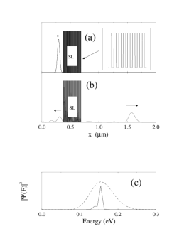
FIG. 3.: The initial probability density $|\psi(z,0)|^{2}$, corresponding to a Gaussian function with $\Delta x=200\,$Å and energy $E=E_{r}=0.155\,$eV, is shown in (a). The potential energy $V_{\text{SL}}(x)$ is plotted as a function of $x$, for a DSL of $N=50$ barriers of $b=32$ Å, whereas the thicknesses of QW are $a=32$ Å  and $a^{\prime}=26$ Å. The inset in (a) is an enlarged view of a portion of the SL potential. The probability density $|\psi(z,t)|^{2}$ at time $t=2\,$ps is shown in (b). The Fourier transform for the initial wave packet (see (a)), $|\psi(E,0)|^{2}$, (dashed line) and for the transmitted packet through the DSL (see (b)) at time $t=2\,$ps, $|\psi(E,t)|^{2}$, (solid line) are shown in (c) as a function of the energy.

We can understand better what is happening by looking at the dynamical evolution of the probability of transmission (reflection) $P_{T}(E,t)$ [$P_{R}(E,t)$], i. e., the probability of finding the particle in the right (left) side of the SL with energy $E$ at time $t$. We notice that the stationary transmission probability $\tau(E)$ which we commented upon in Sec. II is just the limit of $P_{T}(E,t)$,

$$\tau(E)=\,C\,\lim_{t\rightarrow\infty}P_{T}(E,t)$$ (20)

where $C$ is a suitable normalization constant which depends on $\Delta x$ and tends to unity as $\Delta x\rightarrow\infty$. In Figure 4, we plot $P_{T}(E,t)$ and $P_{R}(E,t)$ as a function of time for the resonant energy $E=0.155\,$eV (solid line) and for $E=0.180\,$eV (dotted line) for a DSL, and for $E=0.155\,$eV (dashed line) for a RSL. For a RSL the results are similar for any energy; we have just selected $E_{r}$ as a typical behavior. For the DSL there is a great dependence of the energy. When we select an energy far from the resonant one we have a behavior similar to that the RSL. However, when we choose the resonant one, in a short interval of time $P_{T}$ reaches practically its maximum value. In Fig. 3(b) we can see that this fast enhancement is due to the arrival of a compact packet corresponding to the components of the initial wave with energies closer to $E_{r}$. Again, we have selected a small number of wells to allow an experimental verification of this results, and we have checked that the larger the number of wells is, the larger the differences between RSL and DSL.

FIG. 4.: Dynamical transmission $P_{T}$ (lower curves) and reflection $P_{R}$ (upper curves) probabilities are shown as a function of time for a DSL with the same parameter as in Fig. 3, at energy $E=E_{r}=0.155\,$eV (solid line) and $0.180\,$eV (dotted line) and for a RSL (with the same parameters that de DSL) at energy $E=0.155\,$eV (dashed line). The inset is an enlargement of the transmission probability for a RSL, the lowest curve in the plot.

We are now going to use $P_{T}$ and $P_{R}$ to find approximately the transmission time ($t_{T}$). We will choose the following convention: We obtain the time when the wave packet entries in the SL by finding the maximum value of $\partial P_{R}(t,E)/\partial t$, which indicates the time when the probability of finding the particle inside the SL is maximum, and we will fix our time origin $t_{in}$ at that instant (see Fig. 5). This will be our time origin $t_{in}$. As for the time when the wave packet exits the SL, we can think of it as the time when most of the particles transmitted are on the right part of the SL, i. e., the time $t_{out}$ when $P_{T}$ is arriving to the final plateau (cf. Fig. 5). We obtain $t_{out}$ by finding the maximum value of $\partial P_{T}(t,E)/\partial t$.

If the particle transmitted through the DSL is tunneling through a ballistic channel induced by spatial correlations in the disorder, the packet will pass the same amount of time in each well. Therefore, the time spent by the packet in passing through the whole SL would scale linearly with the number of wells, i. e., the length of the SL. One of the goals of this paper is to show not only that there is a significant enhancement of the transmission probability for particular values of the energy in DSL, but also that we are in the presence of a ballistic transmission phenomenon in a disordered system, very close to the ideal WKB case for periodic SLs. This conclusion can be drawn from Fig. 6. There we have plotted the transmission time as a function of the number of wells, for both types of SL’s, namely RSL and DSL, selecting an energy laying in the DSL mini-band. For comparison, we also show the results predicted by the WKB expression Eq.(10). Remarkably enough, the DSL the behavior is purely linear and very close to that predicted by the WKB expression. On the contrary, for the RSL we have an exponential behavior characteristic of Anderson localized states. It thus becomes well established, from the dynamical view point, the nature of the DSL as a disordered system with good transport properties.

FIG. 5.: We show the typical behavior of the (a) reflection $P_{R}$ and (b) transmission $P_{T}$ probabilities versus time for the resonant energy in a DSL with the same parameters as in Fig. 3. The dashed line represents the derivatives (a) $\partial P_{R}(t,E_{r})/\partial t$ and (b) $\partial P_{R}(t,E_{r})/\partial t$. The arrows mark the maximum values of the derivatives of $P_{R}$ and $P_{T}$, which we take respectively as the initial time $t_{in}$ (i.e. when the wave packet goes inside the SL) and the outside time $t_{out}$ (i.e. when the the wave packet goes out of the SL). The transmission time is defined simply as $t_{T}=t_{out}-t_{in}$.

We now turn our attention to the mean dwell time. When we have a particle situated in an eigenstate, the mean dwell time in the DSL is exactly the transmission time and has a clear relationship with the density of states.[7] On the other hand, if we have a Gaussian wave packet the relation with the density of states is not at all evident. However, if we consider wave packets with small spread in energies we can expect that Eq. 13 continue to hold. In Fig. 7 we have plotted the $t_{dw}$ of an initial Gaussian wave packet of energy $E=E_{r}$ as a function of the number of wells. We can see that for the DSL the behavior is close to the linearity exhibited by the transmission time in Fig. 6 (solid line represents a linear fit). On the contrary, for the RSL the $t_{dw}$ exhibits a plateau because for this kind of SL’s the dwell time is dominated by $t_{R}$. In Fig. 2 we saw that for a RSL most part of the wave packet just penetrates in the SL a small number of wells; therefore $t_{dw}$ does not depend on the SL’s size as soon as the SL is larger than those few wells. This result agrees with the typical consistency check for any definition of tunneling time,[13] where $t_{dw}$ is related to $t_{T}$ and $t_{R}$ by the expression,

$$t_{dw}=(1-\tau)\,t_{R}+\tau\,t_{T}.$$ (21)

For a RSL when the number of wells grows, $\tau$ goes to zero. In this case $t_{dw}$ is equal to $t_{R}$, and hence the plateau observed in Fig. 7.

FIG. 6.: The transmission time $t_{T}$ at the resonant energy as a function of the number of wells $N$ for a DSL (squares) with a linear fit (dashed line) and a RSL (filled circles) with an exponential fit (solid line). Also depicted is the WKB approximation for the DSL case (dot-dashed line), showing a good qualitative agreement (same linear behavior) with the numerical results for the DSL. Parameters for both SL’s are the same as in Fig. 3.

From the preceding considerations and results, we can be confident that in the DSL, when the transmission and dwell times behave similarly and the propagation is quasi-ballistic, the aforementioned relationship between peaks in the density of states corresponding to peaks in the dwell time still holds, the only discrepancy being just a normalization constant, related to the amount of reflected final states. Following this idea, we have plotted in Fig. 8 the density of states, obtained by using Eq. (13). We can see how we have a peak in $t_{dw}$ (and correspondingly in the density of states) for the resonant energy, as was expected for a packet that transmits through the whole SL by using the ballistic channel originated by the spatial correlation in a otherwise disordered SL. We note that this coincides with the predictions from the stationary analysis in Ref. [9], thereby confirming again the results in that paper. In particular, the shape of the density of states curve in Fig. 8 is very similar to that obtained in our previous works.

FIG. 7.: Mean dwell time $t_{dw}$ at the resonant energy as a function of the number of wells $N$, for a DSL (circles) and a RSL (squares). A linear fit for the DSL (solid line) is also shown. Parameters for both SL’s are the same as in Fig. 3.

To conclude this zero field study of the dynamics of DSL’s, we close the section by studying the spreading of the initial wave packet versus time for both kinds of SL’s. In Fig. 9 we have plotted on a log-log scale the mean-square displacement $\sigma$ as a function of time for a wave packet of energy $E=E_{r}$ incident in a DSL (solid line) and in a RSL (dot-dashed line), and for energy $E=0.180\,$eV impinging on a DSL (dashed line). At short times we can see a practically constant behavior of $\sigma$ which can be associated to the period while the wave packet is traveling towards the SL’s. When the packet hits the SL, we see during a short time a decrease of $\sigma$, followed immediately by a rapid increasing of this magnitude. The decreasing is a consequence of the tails of the wave packet reaching the leading part, which is being retained by its collision with the SL; once the whole packet is interacting with the SL, the behavior is close to power-like. We have fitted the results showed in Fig. 9 for times larger than $1$ ps to a function of the form $\sigma(t)\sim t^{\gamma}$. We have obtained for the DSL at the resonant energy $\gamma=1.120$, i.e., we are in a super-diffusive regime, whereas for the DSL away from the resonant energy $\gamma=1.000$, right at the limit between a localized regime and a ordinary diffusive one. Finally, for the RSL $\gamma=0.837$, indicating that we are clearly in a localized regime. The $\sigma$ for the RSL is always much lower than for the DSL and increases with a larger approximate exponent, i. e., after some time ($\sim 1\,$ps) the packet is much more localized for the RSL than for the DSL (even out of the resonance). This is evidently a consequence of localization effects coming from the uncorrelated disorder of the RSL, and whose influence is much less in the DSL case given the availability of extended states. Such a phenomenon further confirms the conclusions we have been drawing all along this section. We will come back to these results in the next section, when dealing with electric field effects.

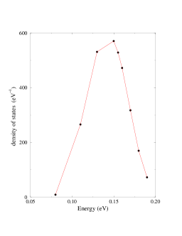
FIG. 8.: Density of states $\rho$ as a function of the incident energy $E$ obtained measuring $t_{dw}$ of a Gaussian wave packet of energy $E$ in a DSL with the same parameters as in Fig. 3. Line is only a guide to the eye.

FIG. 9.: Mean-square displacement $\sigma$ of an initial Gaussian wave packet incident in a DSL at the resonance energy $E_{r}=0.155\,$eV (solid line), and at energy $E=0.180\,$eV (dashed line) and for a RSL at energy $E=0.155\,$eV (dot-dashed line). Parameters for both SL’s are the same as in Fig. 3. Note the log-log scale.

IV Electric field effects

The zero field simulations we have been presenting provide an incomplete picture of electron dynamics in DSL’s, as in this case it is obvious that technologically applicable phenomena would involve electric fields. Therefore, in this section we study the dependence of the dynamical characteristics discussed in the previous paragraphs on an electric field. In Sec. II we explained that the subband of extended states appearing in DSL’s is shifted to lower energies and reduces its width in the presence of moderate electric fields. We want to confirm that the correspondingly shifted quasi-bound states will have time enough to be established in the dynamical interaction of a Gaussian wave packet with a DSL potential when there is an applied field. To this end, in Fig. 10 we have plotted $P_{T}$ for a Gaussian wave packet incident on a DSL with $E=0.155\,$eV, for different values of the electric field $F$.

FIG. 10.: Transmission probability $P_{T}$ as a function of time for a DSL with the same parameters as in Fig. 3, at energy $E=E_{r}=0.155\,$eV, for different values of the electric field $F=1\,$kV/cm (dashed line) and $5\,$kV/cm (dot-dashed line). For comparison we also show the result for $F=0$ (solid line).

We can see that, at least for moderate fields, the dwell time is large enough ($t_{dw}\simeq\hbar/\Gamma$) to allow the quasi-bound states to be established thus permitting the transmission of the resonant components of the packet. The maximum value of $P_{T}$ decreases with the field due to the shift of the mini-band and because the miniband becomes much narrower the larger the electric field applied is. Interestingly, we can still find a dynamical resonant energy looking at the Fourier transform of the transmitted wave packet, as shown in Fig. 11. We want to stress that these results can be of interest for applications, because a DSL turns out to be a structure that works like an adaptive electronic filter, namely, by tuning properly the SL parameters we can filter the energies contained in a narrow band. Moreover, this band can be displaced to the desired values by selecting a particular value of the applied electric field.

FIG. 11.: The Fourier transform for the transmitted packet versus energy in the presence of an electric field $F=10\,$kV/cm (dashed line); solid line shows the result at zero field. The insets show the transmission coefficient $\tau$ as a function of energy for the two values of the electric field $F$ for reference. The SL parameters are the same as in Fig. 3

There is another aspect of the influences of electric fields on electron dynamics which is worth considering, namely the following: It is well known that, when an electric field is applied to a periodic SL, the localization of the initially extended states produces an oscillatory behavior of the wave packet, the so-called Bloch oscillations. Of course, Bloch oscillations require a quasi-perfect quantum coherence and a perfectly defined phase to be self-sustained in time. This is not the case in a DSL where electronic states increment their phase by a factor $\pi$ whenever they pass over a DQW. [2] The question then arises as to what will the corresponding phenomenology in this case be. In order to answer this question, in Fig. 12 we plot the IPR, defined in Eq. (III B), as a function of time for (a) a perfect SL, (b) a DSL and (c) a RSL, in the presence of an electric field. The initial condition of these simulations was that, at $t=0$, we placed a Gaussian wave packet with an energy of $E=0.155\,$eV and $\Delta x=20\,$Å in the center of each one of those SL’s with $50$ wells. In our case $F=10\,$kV/cm, $d=a+b=64\,$Å. In an ordered SL, the Bloch period will then be $T_{\text{Bloch}}=h/eFd\sim 0.646\,$ps, in perfect agreement with obtained from Fig. 12(a). For the disordered superlattices there is an oscillatory behavior at the beginning but in a short time the IPR achieves a randomly fluctuating, but stationary in mean, value. This indicates the existence of decoherence effects in both disordered lattices, the difference between the RSL and the DSL being that the latter shows a smaller mean value of the IPR, in agreement with the less localized character of its states. The remnants of oscillatory behavior for the disordered SL’s are more clearly characterized by looking at the mean square displacement $\sigma$ as a function of the time, which is shown in Fig. 13. Again, we can see how in the DSL the wave packet is much more delocalized that in the RSL as a consequence of the presence of a narrow band of extended states.

FIG. 12.: IPR of an initial Gaussian wave packet placed in a (a) perfect SL, (b) DSL, and (c) RSL as a function of time. For the three kind of SL’s, the number of wells is $N=200$ and the rest of parameters are the same as in Fig.3.

FIG. 13.: Mean-square displacement $\sigma$ of an initial Gaussian wave packet placed in a DSL (solid line) and RSL (dashed line), in the presence, of an electric field $F=10\,$kV/cm, as a function of time. SL parameters are the same as in Fig. 12

V Discussion and Conclusions

In this work we have successfully shown that the good transport properties predicted by previous static studies of SL’s with correlated disorder give rise to corresponding dynamical phenomena of interest. To this end, we have reported on dynamical properties of electrons in intentionally disordered SL’s, computed by using high-accuracy numerical methods to solve the time dependent Schrödinger equation for the complete Hamiltonian. In this respect, as the two main global conclusions of the present paper, we want to stress, first, that the dynamical results we show prove independently the existence of extended states with physical consequences in disordered systems, and second, that the validity of our previous static calculations in Refs. [4] and [9] to characterize electron transmission through nanostructures has been set on firm grounds due to its perfect agreement with the dynamical analysis.

Aside from the above general conclusion, which we draw from the consideration of a number of dynamical tools, we would like to summarize a few aspects more that we have learned from our simulation program. In particular, we have proposed a method to find the transmission time by using the temporal transmission probability, provided that such probability presents abrupt changes as a function of time. By means of this procedure to compute the transmission time, we have been able to show that the propagation of electrons with energies in the subband of extended states of a DSL is ballistic, very similar to that of ordered SL’s. This is a dramatic manifestation of delocalization by correlations, more so when compared to the exponential growth of the transmission time we have obtained for usual RSL’s. In that regime, we have shown that the relationship between dwell times and density of states, holds for Gaussian wave packets, by computing the density of states and finding the same result as in our stationary calculations. Interestingly, the fact that correlations do not impede the phase decoherence of the wavepacket, the properties depending on symmetries of the system (translational invariance) are not recovered. This is the case, e. g., of Bloch oscillations. In any event, measurements of the IPR point out once more the differences between DSL’s and RSL’s. All this characterization is confirmed by measuring the mean square displacement of electrons, which are seen to evolve faster in DSL’s. Finally, we have also confirmed that low to moderate electric fields do not destroy the transport properties of DSL’s, which is very important if DSL’s are to be built and used for any practical purpose.

To conclude, a few words are in order regarding possible applications of the present work. It seems quite clear to us that several of our results can be useful for nanotechnological devices with specific, special features. To begin with, the great difference of transmission times between extended states and localized ones may provide a powerful tool for measure the extended character of the states in open systems. Besides, it can also be used to measure the amount and character of the disorder inherently present in any periodic SL, by obtaining the width of the band of extended states in the actual SL and comparing it to the theoretically predicted one. However, what we think by far is the most promising application of DSL in nanotechnology has to do with their filter-like behavior. We have seen that it is possible, by means of an applied electric field, to control the center and width of the band of extended states, therefore allowing for a tunable filtering of wavepackets, i. e., of electrons. This capability, present already in practically achievable DSL’s of some 50 wells, can be used to design a new family of electronic devices. In this respect, it is quite clear that a natural extension of this work would be to study the interaction of RSL and correlated disordered SL’s, with an AC-electric field, using the complete Hamiltonian. Preliminary tight-binding results [15] appears to show exciting new phenomena in these structures. We envisage that appropriate choices of the frequency and/or intensity of the field can give rise to crucial changes in the filtering properties of DSL’s. Further work along these lines is currently in progress. [16]

- [1] A. Sánchez, F. Domínguez-Adame, G. Berman, and F. Izrailev, Phys. Rev. B 51, 6769 (1995).
- [2] A. Sánchez and F. Domínguez-Adame, J. Phys. A 27, 3725–3730 (1994).
- [3] J. M. Ziman, Models of Disorder (Cambridge University Press, London, 1979).
- [4] E. Diez, A. Sánchez and F. Domínguez-Adame, IEEE J. Quantum Electron. 31, 1919 (1995).
- [5] M. Büttiker and R. Landauer, Phys. Rev. Lett. 49, 1739 (1982).
- [6] G. P. Berman, E. N. Bulgakov, D. K. Campbell and A. F. Sadreev, Phyisica B in press (1996).
- [7] G. Iannaccone, Phys. Rev. B 51, 4727 (1995).
- [8] E. E. Mendez and G. Bastard, Physics Today, June, 34 (1993).
- [9] F. Domínguez-Adame, A. Sánchez and E. Diez, Phys. Rev. B 50, 17 736 (1994).
- [10] R. Knapp, G. Papanicolaou, and B. White, J. Stat. Phys. 63, 567 (1991).
- [11] See W. H. Press, B. P. Flannery, S. A. Teukolsky, and W. T. Wetterling, Numerical Recipes: The Art of Scientific Computing (Cambridge University Press, New York, 1986) pp. 656-663
- [12] A. M. Bouchard and M. Luban, Phys. Rev. B 52, 5105 (1995).
- [13] G. Iannaccone and B. Pellegrini, Phys. Rev. B 49, 16 548 (1994).
- [14] S. N. Evangelou and D. E. Katsanos, Phys. Lett. A 164, 456 (1992).
- [15] M. Holthaus, G. H. Ristow, and D. W. Hone, Phys. Rev. Lett. 75, 3914 (1995).
- [16] E. Diez, A. Sánchez, F. Domínguez-Adame, and G. P. Berman (unpublished).