Universal Cubic Eigenvalue Repulsion for Random Normal Matrices

Abstract

Random matrix models consisting of normal matrices, defined by the sole constraint $[{\bf N}^{{\dagger}},{\bf N}]=0$, will be explored. It is shown that cubic eigenvalue repulsion in the complex plane is universal with respect to the probability distribution of matrices. The density of eigenvalues, all correlation functions, and level spacing statistics are calculated. Normal matrix models offer more probability distributions amenable to analytical analysis than complex matrix models where only a model with a Gaussian distribution are solvable. The statistics of numerically generated eigenvalues from gaussian distributed normal matrices are compared to the analytic results obtained and agreement is seen.

I Introduction

Random matrix theory (RMT), [2], [3] has found much success as phenomenological models describing a wide variety of physical systems, from discretization of moduli space [4], to the statistics of the cells in the skin of a cucumber [5]. RMT is the study of eigenvalues derived from random ensembles of matrices with stochastic elements specified by a probability density, $P({\bf M})d{\bf M}$, in the space of matrices. Most interest is in examining the properties of the eigenvalues induced from the transformation to the eigenvalue basis. Early work consisted of using real symmetric, hermitian, unitary, and real quarternion matrices [6]. The eigenvalues of which are either real or unimodular, (and termed one dimensional eigenvalues here).

Recently several groups have begun to consider physical applications of matrix models composed of complex matrices. Introduced in the early sixties by Ginibre [7] it took decades for others to consider applications. As the probability distribution is not invariant under similarity transformations the diagonalizing parameters must be integrated out by brute force. It was found that only a distribution with a gaussian weight (Ginibre Ensemble) could be solved. The Ginibre ensemble was later found to exhibit cubic eigenvalue repulsion in the complex plane, [8] [3]. Such models are of interest in characterizations of quantum chaos. Cubic quasi-energy level repulsion is a key signature of classical chaos within a quantum dissipative system, as defined by Haake [8].

Normal matrices are discussed in most matrix theory texts, (see [9], [10]). Defined by the sole constraint that they commute with their adjoint, they have the property of being the most general matrix that can be diagonalized by a unitary transformation. The normal matrix model was first introduced in showing how the Laughlin wavefunction could be modeled by it and offered some generalizations to inhomogeneous fields [11]. In [12] the statistics of eigenvalues of random normal matrices were first explored.

In this paper the universality of cubic eigenvalue repulsion in the complex plane for ensembles of random normal matrices will be shown. In section II the probability distribution in the space of matrices, all correlation functions, and the eigenvalue densities will be obtained. In section III the level spacing statistics of the eigenvalues obtained will be derived. The term level spacing is borrowed from the Wigner-Dyson ensembles and will represent here the spacing in the complex plane. In section IV eigenvalues of numerical generated normal matrices will be studied and compared to the analytical results.

II Probability Distributions, N-pt. Correlation Functions

We begin by defining the joint probability distribution (jpd) within the space of normal matrices,

$$P_{N}({\bf M}) = C\exp[-Tr(V({\bf M},{\bf M}^{{\dagger}}))].$$ (1)

Only potentials which are hermitian will be considered, $V({\bf M},{\bf M}^{{\dagger}})=V({\bf M},{\bf M}^{{\dagger}})^{{\dagger}}$. As a result the joint probability distribution for the eigenvalues will be rotationally symmetric in the complex plane. Normal matrices are the most general matrices which can be diagonalized by a unitary transformation, $\bf{M}=\bf{UZU^{{\dagger}}}$, so that the measure and the weight are invariant. Thus it is simple to derive the jacobian for the transformation to the eigenvalues.

Proceeding analogously to the hermitian matrix case [13], the metric in the space of normal matrices is defined as,

$$(ds)^{2} = Tr[\bf{dM^{{\dagger}}dM}]$$ (2)

$$= Tr(\bf{Ud(U^{{\dagger}}ZU)U^{{\dagger}}Ud(U^{{\dagger}}Z^{\ast}U)U^{{\dagger}}})$$ (3)

$$= Tr(\bf{[dS,Z][dS,Z^{\ast}]}+(\bf{[dS,Z]dZ^{\ast}}+\bf{dZ[dS,Z^{\ast}]})+|\bf{dZ}|^{2})$$ (4)

$$= c\sum_{i<k}|dS_{ik}(z_{k}-z_{i})|^{2}+\sum_{i}|dz_{i}|^{2},$$ (5)

where $\bf{dS}=\bf{UdU^{{\dagger}}}=-\bf{dUU^{{\dagger}}}$ is antihermitian and $c$ is an overall constant.

Using the standard Riemannian volume form with this metric we get,

$$d\mu({\bf M})\longrightarrow d\mu(z)=(d\Omega)|\Delta(z)|^{2}dz^{(0)}_{1}\wedge dz^{(0)}_{2}\wedge...\wedge dz^{(0)}_{N}\wedge dz^{(1)}_{1}\wedge...\wedge dz^{(1)}_{N}.$$ (6)

where $d\Omega$ is the volume of the unitary group $U(N)$, and $\Delta(z)$ is the well known Van der Monde determinant,

$$|\Delta(z)|^{2} = \prod_{i<j}^{N}|z_{j}-z_{i}|^{2}$$ (7)

If we consider weights which are invariant under unitary transformations we can factor $d\Omega$ out,

$$P_{N}(z) = C^{\prime}|\Delta(z)|^{2}\exp[-\sum_{i=1}^{N}V(z_{i},z_{i}^{\ast})],$$ (8)

where $C^{\prime}$ is a normalization constant.

Considering a gaussian weight, $V=|z|^{2}$, we notice that the jpd is identical to Ginibre’s ensemble of complex matrices[7]. The model with this weight function is termed the Normal Gaussian Ensemble (NGE). It is clear that gaussian ensembles of complex matrices and the NGE are identical. Any result derived here for the NGE will also be valid for Ginibre’s ensemble of matrices. This is of little surprise since $Tr[{\bf M}^{{\dagger}}{\bf M}]=Tr[{\bf M}{\bf M}^{{\dagger}}]$.

The difference occurs when considering other ensembles. For complex matrices the parameter $\beta$, (defined as the power of the Van der Monde determinant appearing in the jpd), is a function of the weight. In fact, only models involving gaussian weights have ever been studied as this is the only nontrivial model which allows a separation of radial and angular parameters. For normal matrices $\beta=2$ regardless of the weight and it is possible to study a wide variety of ensembles.

For matrix models with one dimensional eigenvalues the traditional method of analysis employs a basis of orthogonal polynomials. These allow the reduction of the determinant upon integration of a number of eigenvalues [3]. For complex eigenvalues we can also introduce an orthogonal basis. If a polar basis is chosen, (and $P_{N}(z)$ is rotationally symmetric), it is simple to verify that the $z$’s themselves form an orthogonal basis. A basis of orthogonal monomials, $\{\phi\}$, is defined,

$$\phi_{l}(z_{i}) \equiv {z_{i}^{l}\over N_{l}^{1\over 2}},$$ (9)

where $N_{l}=\int_{0}^{\infty}dr^{2}r^{2l}\exp[-V(r)]$, is a normalization constant.

The jpd can then be expressed as,

$$P_{N}(z) = C^{\prime}e^{-\sum_{i=1}^{N}V(z_{i},z_{i}^{\ast})}detK_{N}(z_{i},z_{j})|_{i,j=1,N},$$ (10)

where the “kernel” is,

$$K_{N}(z_{i},z_{j}) = \sum_{l=0}^{N-1}\phi_{l}(z_{i})\phi_{l}^{\ast}(z_{j}).$$ (11)

The weight function is deliberately factored out of the kernel since all of the angular dependence is contained within $K$.

Similarly to hermitian matrix models, when $N-n$ eigenvalues are integrated out of the jpd, the determinant shrinks by $N-n$ columns and rows, [12]. This property allows the $n$-point correlation function to be derived easily,

$$R_{n}(z_{1},\cdots,z_{n}) \equiv {N!\over(N-n)!}\int\prod_{i=n+1}^{N}{1\over 2}d\theta_{i}dr_{i}^{2}P_{N}(z),$$ (12)

$$= e^{-\sum_{i=1}^{n}V(r_{i})}detK_{N}(z_{i},z_{j})|_{i,j=1,n}.$$ (13)

The prefactor ${N!\over(N-n)!}$ is due to the ordering of eigenvalues. The 2 point correlation function and eigenvalue density are,

$$R_{2}(z,w) = {e^{-V(z)-V(w)}\over\pi^{2}}[\rho(z)\rho(w)-K(z,w)K(w,z)],$$ (14)

$$\rho(z) = e^{-V(z)}\sum_{l=0}^{N-1}{|z|^{2}\over N_{l}},$$ (15)

In deriving expressions for the correlation functions orthogonal monomials provide a more economical method. However, there are no simple recursion relations among the monomials as there are for the orthogonal polynomials. No recursion relation implies no Christoffel-Darboux formula and no asymptotic analysis. However, we can find analytical results for finite $N$. It is not necessary to examine the asymptotic form of the monomials to get large $N$ forms.

In table I various ensembles are defined and their corresponding eigenvalue density and two point correlation function are given. It should be noticed that several of these ensembles allow global closed forms in the limit $N\rightarrow\infty$.

III Level Spacing Statistics

In order to study the properties of random matrices the statistical properties of the spacings between eigenvalues, (or level spacings), are examined. These statistics can be used as a definition of quantum chaos. The distinction of classically integrable and chaotic systems can be seen in a semiclassically quantized system as the transition from Poisson to Wigner-Dyson statistics of the nearest neighbor distribution of the energy levels [14]. It has been shown [8] that if there is dissipation in the system the level spacings undergo a similar transition from a Plane Poisson distribution, (random points in a plane), to Ginibre’s distribution [7] generated by an ensemble of random complex matrices.

The distributions for eigenvalues in the complex plane will require the definition of statistical quantities analagous to those defined for Hermitian matrix models [3].

• The probability that no eigenvalue lies within a circle of radius $s$ centered upon the point $w$, the gap distribution, is denoted as $E(s,w)$. A related quantity $E(s,w,\epsilon)$ is defined as the probability that no eigenvalues lie within an annulus of outer radius $s$, inner radius $\epsilon$, and centered on the point $w$.

• The probability that no eigenvalues lie within this same circle but one or more eigenvalues lying on the perimeter is denoted as $F(s,w)$.

• For an eigenvalue lying at the center of the circle and no eigenvalues within the circle nor on the edge, this probability is denoted by $H(s,w)$.

• The level spacing probability, $p(s,w)$, is the most quoted quantity and is defined as the probability that one eigenvalue lies at the center and one ormore on the perimeter.

By taking differential areas at the center and at the perimeter of this circle, we can obtain all of the probabilities from the gap distribution. The argument is analagous to Mehta’s for one dimensional eigenvalues and can be found in [12].

$$E(s,w) = \int\{dz\}P_{N}(\{z\})\prod_{i=1}^{N}[1-\chi(z_{i},s,w)],$$ (16)

$$F(s,w) = -{d\over ds}E(s,w)$$ (17)

$$H(s,w) = -{d\over d\epsilon^{2}}E(s,w,\epsilon)|_{\epsilon=0}$$ (18)

$$p(s,w) = -{d\over ds}H(s,w)=$$ (20)

$$-{d\over d\epsilon^{2}}F(s,w,\epsilon)|_{\epsilon=0}={d\over ds}{d\over d\epsilon}E(s,w,\epsilon)|_{\epsilon=0}.$$

Where, $\chi$ is the characteristic function and $\epsilon$ is taken as the radius of an infinitesmal area centered at the center of the circle. These relations allow an elegant derivation of the level spacing distribution.

All of the probability distributions considered here are symmetric in the $z_{i}$, hence the derivation of the gap distribution will be the same as in [3], (see also [12]). For the circle centered at the origin we have the following,

$$E(s,0) = \prod_{i=0}^{N-1}\left[{\int_{s^{2}}^{\infty}dx\exp(-V(x))x^{j}\over\int_{0}^{\infty}dx\exp(-V(x))x^{j}}\right],$$ (21)

where $x=|z|^{2}$.

As a check on our results, we find the spacing distribution for the NGE and compare with previously known results. In this case the probability distribution is translationally invariant, hence the result (21) is valid for all $w$. The result for small $s$ is,

$$p(s)\approx 2s^{3}-s^{5}+{1\over 7}s^{7}-{11\over 12}s^{9}\cdots$$ (22)

This result is the same as for complex matrices derived by Haake[8]. The level spacing statistics at the origin for other ensembles of normal matrices can be found in [12]. Here we are concerned with obtaining a universal result for the spacing distribution.

For ensembles other than Gaussian, the distributions are not translationally invariant and hence it will be necessary to resort to asymptotic approximations. Shifting the eigenvalue coordinate, $z=z-w$, does not affect the measure or Van der Monde determinant. The gap distribution can then be expressed as,

$$E(s,w) = \prod_{i=1}^{N}\int_{0}^{\infty}dr_{i}^{2}d\theta_{i}[1-\chi_{i}(s^{2})]{\tilde{P}}_{N}(z),$$ (23)

$$= \int_{0}^{\infty}\{d^{2}z\}\{1-\sum_{i=1}^{N}\chi_{i}(s^{2})+\sum_{i\neq j=1}^{N}\chi_{i}(s^{2})\chi_{j}(s^{2})-\cdots\}{\tilde{P}}_{N}(z),$$ (24)

$$= 1-\sum_{i}^{N}\int d^{2}z_{i}\chi_{i}\tilde{\rho}(z_{i})+\sum_{i\leq j}^{N}\int d^{2}z_{i}d^{2}z_{j}\chi_{i}\chi_{j}{\tilde{R}}_{2}(z_{i},z_{j})-\cdots,$$ (25)

where $\tilde{f}(z)=f(z-w)$ and $\chi_{i}$ is the characteristic function for the $i^{th}$ eigenvalue. In the limit $s\rightarrow 0$, and keeping only the first two terms we obtain,

$$\lim_{s\rightarrow 0}E(s,w) \approx 1-N\pi s^{2}\rho(w).$$ (26)

The level spacing distribution, $p(s,w)$, can be found via equation (20). First the gap distribution $E(s,w,\epsilon)$ needs to be derived. The derivation is the same as before except for a modification to the characteristic function. Starting from (25) we have,

$$E(s,w,\epsilon) = 1-\sum_{i}^{N}\int d^{2}z_{i}\chi_{i}\tilde{\rho}(z_{i})+\sum_{i\leq j}^{N}\int d^{2}z_{i}d^{2}z_{j}\chi_{i}\chi_{j}{\tilde{R}}_{2}(z_{i},z_{j})-\cdots,$$ (27)

where now $\chi_{i}=\theta(s^{2}-r_{i}^{2})\theta(r_{i}^{2}-\epsilon^{2})$. As an intermediate step we find,

$$H(s,w) = -{d\over d\epsilon^{2}}E(s,w,\epsilon)|_{\epsilon=0},$$ (28)

$$= N{d\over d\epsilon^{2}}\int_{\epsilon^{2}}^{s^{2}}dr^{2}\int d\theta\rho(z+w)$$ (30)

$$\qquad-{N^{2}+N\over 2}{d\over d\epsilon^{2}}\int_{\epsilon^{2}}^{s^{2}}\int_{\epsilon^{2}}^{s^{2}}{dr_{1}^{2}dr_{2}^{2}\over 4}\int\int d\theta_{1}d\theta_{2}R_{2}(z_{1}+w,z_{2}+w)+\cdots|_{\epsilon=0},$$

$$= -N\pi\rho(w)+\pi(N^{2}+N)\int_{0}^{s^{2}}{dr_{2}^{2}\over 2}\int d\theta_{2}R_{2}(w,z_{2}+w)-\cdots.$$ (31)

The last term exploits the symmetry in $R_{2}$. For the level spacing we have,

$$p(s,w) = -\pi(N^{2}+N)s\int d\theta_{2}R_{2}(w,se^{i\theta_{2}}+w)\cdots$$ (32)

In order to find the lowest order contribution to $p(s,w)$ the lowest order of $R_{2}$ will need to be found. For a model with weight $e^{-V(z)}$ we have,

$$R_{2}(w,z+w) = e^{-V(w)}e^{-V(z+w)}\sum_{l=1}^{N}\sum_{m=0}^{N}[{r_{w}^{2l}(r^{2}+zw^{\ast}+wz^{\ast}+r_{w}^{2})^{m}\over N_{l}N_{m}}-{(zw^{\ast}+r_{w}^{2})^{l}(wz^{\ast}+r_{w}^{2})^{m}\over N_{l}N_{m}}].$$ (33)

The normalization factor, $N_{l}$ is model dependent. It is easily verified that terms with $l=0$ and $l=m$ vanish. All higher order functions will have the same property.

The remaining angular integral over $d\theta_{2}$ in (32) insures that no terms linear in $z$ or $z^{\ast}$ appear. It is also apparent that the leading term in $r_{w}$ cancels, (terms to order $z^{0}$). This yields the lowest order of $R_{2}$ to be $s^{2}$. Combined with equation (20), it is found that the nearest level spacing is cubic in $s$ as $s\rightarrow 0$. A few exceptions occur when the weight function vanishes as $z$ vanishes. Specifically the Jacobi, Laguerre, ($a>1$) and generalized Gaussian ($a>1$) will have a higher order repulsion. Our final result is thus:

Normal matrix models with normalizable hermitian weight functions have eigenvalues experiencing a minimum of cubic repulsion in the complex plane.

It is also worthwhile to examine the case of real normal matrices. Here the constraint being that the matrix commutes with its transpose. Such a matrix is diagonalizable by a unitary transformation and will in general have complex eigenvalues. Retracing the steps above it is easy to see that the eigenvalues will also exhibit a minimum of cubic repulsion in the complex plane.

IV Numerical Results

Whenever discussing random matrix theory it is always of interest to include numerical simulation of large random matrices. These are used to verify the analytical properties and supply support for asymptotic forms, conjectures, etc. When dealing with normal matrices however, we are in a predicament. Consider the following problem:

• Write down an arbitrary $2\times 2$ normal matrix that is not Hermitian, Unitary, nor Real.

It is not so simple. If one was asked to write down a hermitian matrix, it could be done without thinking twice. For a normal matrix there is no simple parameterization. It would most likely require the commutator to be calculated and a solution found by trial and error. Likewise, if you want a computer to generate normal matrices you must give it a parameterization. For a $2\times 2$ you can parameterize it as follows, given that ${n_{11}}^{\ast}\neq{n_{22}}^{\ast}$, (remember there are $N^{2}+N=6$ independent real elements within a normal matrix),

$${\bf N} = \left(\matrix{n_{11}&n_{12}\cr n_{12}^{\ast}({n_{11}-n_{22}\over n_{11}^{\ast}-n_{22}^{\ast}})&n_{22}\cr}\right).$$ (34)

For arbitrary $N$ the constraint equations become nonlinear and highly coupled. We will choose the following parameterization of normal matrices, define the independent elements as $n_{ij}$, (those along the diagonal and above the diagonal). Define the elements that are constrained as $f_{ji}$, (those which lie below the diagonal). For the $ji^{th}$ element the constraint equation is,

$$f_{ji} = {1\over(n_{jj}^{\ast}-n_{ii}^{\ast})}\left[n_{ij}^{\ast}(n_{jj}-n_{ii})+\sum_{k=1}^{i-1}n_{kj}^{\ast}n_{ki}-\sum_{m=j+1}^{N}n_{im}^{\ast}n_{jm}\right]$$ (36)

$$-{1\over(n_{jj}^{\ast}-n_{ii}^{\ast})}\left[\sum_{k=1}^{i-1}f_{jk}f_{ik}^{\ast}-\sum_{m=j+1}^{N}f_{mi}f_{mj}^{\ast}-\sum_{l=i+1}^{j-1}(n_{lj}^{\ast}f_{li}-n_{il}^{\ast}f_{jl})\right].$$

Notice that the term in the first bracket contains only independent elements. With this parameterization the probability of obtaining normal matrices which are hermitian, unitary, orthogonal, or real symmetric matrices becomes infinitesimal for large $N$. The subspaces for these types of matrices within the space of normal matrices are of much lower dimensionality. There are many solutions to this nonlinear equation. Another method must be devised to obtain a normal matrix. It is also found that due to the nonlinearity, only normal gaussian matrices can be generated. (Others not respecting the hermiticity and normalizibility could be analyzed but is not of interest here).

Instead of directly attempting to produce random normal matrices we begin with a random complex matrix and use an optimization algorithm to obtain a normal matrix. The following algorithm is the simplest to implement but by no means the most efficient.

1. Parameterize the normal matrix as before:
   Elements along the diagonal and above the diagonal are independent parameters. Elements below the diagonal will be optimized.

2. Using the Box-Muller technique, generate random gaussian variables and construct a $200\times 200$ complex gaussian matrix. This is the initial condition.

3. Calculate the commutator and define the following error function, $tr[{\bf N,N^{\dagger}}]^{2}=E$. The error function will be minimized below a choosen threshold, (a value of 0.2 is used).

4. Use gradient descent to adjust the constrained elements. If the value of $E$ is below the choosen threshold then pass the matrix to the diagonalization routine. If $E$ hasn’t converged after 500 iterations, then reset the matrix and go to step 2.

The results of a preliminary numerical study based on this algorithm are now presented. A full discussion of the algorithm used is to be found elsewhere, [12]. Due to limited computational resources and time, only 50 matrices of size 200 $\times$ 200 have been analyzed. The level spacing statistics for the generated matrices is compared to the analytical result.

Before attempting to generate large normal matrices the algorithm was checked with $2\times 2$ matrices. As these were easily produced, 11,000 were generated and compared to the exact analytical result,

$$p_{2\times 2}(s) = {{\pi^{2}s^{3}}\over 10.4683}e^{-{1\over 4}s^{2}}I_{0}({s^{2}\over 4}).$$ (37)

The eigenvalues are unfolded so that the mean spacing is unity, this is achieved by rescaling the spacing and renormalizing the spacing distribution so that the mean spacing between eigenvalues is unity,

$$S \equiv 1.6622s,$$ (38)

$$p(S) \equiv p(s)/10.4883.$$ (39)

Plots of the analytical form and the unfolded eigenvalues are displayed in figure 1.

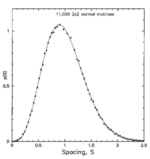
FIG. 1.: The level spacing distributions, p(S), for $N=2$, analytical form and 11,000 numerically generated normal matrices.

For normal matrices of size $200\times 200$ the exact analytical form for the spacing distribution can easily be found from equations (16)-(20),

$$p_{200}(s) = (199-\sum_{q=1}^{199}{e_{q-1}(s^{2})\over e_{q}(s)})2s\prod_{i=1}^{199}\left[e^{-s^{2}}e_{i}(s^{2})\right],$$ (40)

where $e_{q}(s^{2})=\sum_{l=0}^{q}{s^{2l}\over l!}$. Under the optimization algorithm it is found that many eigenvalues “leak” out into the complex plane. Adding a further constraint to keep the eigenvalues within a radius of $\sqrt{2\sigma N-1}\approx 20$ lengthens the generation time dramatically. Therefore, for this preliminary study the eigenvalues were “pruned”, those falling outside $r=18.1$ were neglected, (the number was choosen so that edge effects would be eliminated as well). Overall, about one third of the eigenvalues were pruned. The results are displayed in figure 2.

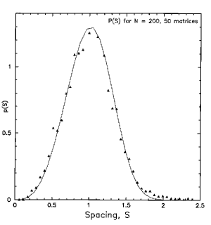
FIG. 2.: The level spacing distributions, p(S), for $N=200$, analytical result (with eigenvalues unfolded), and 50 numerically generated $200\times 200$ normal matrices.

The slight deviation of the numerical and analytical results for large $S$ is due to the leakage of eigenvalues. The small $S$ behavior is not affected by the leakage. It is found that changing the initial conditions has little effect on $p(S)$. It is also observed that lowering the the threshold for the error function by a factor of ten has a negligible effect.

V Conclusion

It has been shown that cubic repulsion of eigenvalues obtained from random normal matrices experience a minimum of cubic repulsion in the complex plane. Even though normal matrices are subsets of complex matrices we have demonstrated that Gaussian normal matrix models yield the same results as the Ginibre ensemble of complex matrices. One can define ensembles of complex matrices with weights invariant under similiarity transformations, (see appendix B of [12]). These ensembles will fall under the $\beta=4$ and experience a minimum of quartic repulsion. (Getting analytical results for the statistics of the eigenvalues is difficult however). Ensembles of complex matrices with weight functions invariant under unitary transformations other than the Gaussian are not factorable and are not amenable to analytical analysis. For normal matrices we can define identical ensembles to complex models invariant under similiarity transformations and as well define a wide range of ensembles invariant under unitary transformations, (as demonstrated in this paper). The special case of real normal matrices was also shown to experience cubic repulsion in the complex plane. As well, there are even more significant differences between random normal matrices and, more traditional, random matrix models composed of hermitian, unitary, and real symmetric matrices, themselves being subsets of normal matrices. Although numerical generation of normal matrices is not as straightforward as for other types of matrices we have shown that analytical results are often much easier to obtain. What numerical information we could obtain does agree with the theoretical result.

It is a little disappointing that universality, in the sense of Brezin and Zee [15], is not found for normal matrix models. The simple scaling arguments that lead to universal kernels for other types of matrices do not work here. It may be possible to rescale $S$ to obtain a universal spacing distribution $P(S)$. This allows the potential of analytically exploring the statistics of complex eigenvalues which was not possible before. Another interesting feature is the closed form expressions for the two point correlation functions in NGE, Laguerre ($a=0$), and Legendre ensembles in the infinite matrix limit, (see Table I).

In terms of physical applications it should be noted that results using the Ginibre ensemble of complex matrices can be duplicated with the normal Gaussian ensemble. Such work includes, modeling cellular structures by Le Caer and Ho [5], two dimensional quantum gravity by Morris [16], and Haake’s work on generators of quantum dynamics for systems with dissipation [8]. It has recently been shown, [17], that Haake’s generator of dissipation, $D$, in [18] [8], is properly represented by a normal matrix rather than a complex one. This result strengthens the idea that the eigenvalues of these generators universally exhibit cubic repulsion when dissipative dynamics is present.

The results obtained in this work give a more complete picture of the statistics of eigenvalues from random matrices. The normal matrix model, a link between the Dyson ensembles and the Ginibre ensemble, has a rich structure where interesting results can still be found.

TABLE I.: Ensembles of random normal matrices defined by their probability distribution. Also shown are the corresponding eigenvalue density and two point function. For the NGE, Laguerre $a=0$, and Legendre ensembles the closed form large $N$ result has been shown.

Ensemble	Probability Distribution	Density, $\rho$	$\rho(r_{1})\rho(r_{2})-R_{2}$
NGE	$e^{-Tr{\bf M^{{\dagger}}M}}$	${1\over\pi}$	${1\over\pi^{2}}\exp[-|z-w|^{2}]$
NQE	$e^{-Tr({\bf M^{{\dagger}}M}-g{\bf M^{{\dagger}}M^{{\dagger}}MM})}$	${e^{-r^{2}-gr^{4}}\over\pi}\sum_{l=0}^{N-1}{r^{2l}\over N_{l}(g)}$	${e^{-r_{1}^{2}-r_{2}^{2}-gr_{1}^{4}r_{2}^{4}}\over\pi^{2}}K_{N}(z_{1},z_{2})K_{N}(z_{2},z_{1})$
Laguerre	$e^{-Tr(({\bf M^{{\dagger}}M})^{1\over 2}+{a\over 2}\ln({\bf M^{{\dagger}}M}))}$	${e^{-r}r^{a+1}\over 2\pi}\sum_{l=0}^{N-1}{r^{2l}\over\Gamma[2l+a+2]}$	$\sum_{l=0}^{N-1}{(r_{1}r_{2})^{a+1}e^{-r_{1}-r_{2}}z_{1}^{l}{z_{2}^{\ast}}^{l}{z^{\ast}}_{1}^{m}z_{2}^{m}\over 4\pi^{2}\Gamma[2l+a+2]\Gamma[2l+a+2]}$
Laguerre, $a=0$	$e^{-Tr({\bf M^{{\dagger}}M})^{1\over 2})}$	${e^{-r}\over 2\pi r}\sinh(r)$	${e^{-r_{1}-r_{2}}\over 4\pi^{2}r_{1}r_{2}}\sinh(\sqrt{z_{1}z_{2}^{\ast}})\sinh(\sqrt{z_{1}^{\ast}z_{2}})$
Legendre	1, (evals $\in$ unit circle)	${1\over\pi(1-r^{2})^{2}}$	${1\over\pi^{2}}\left[{1\over(1-z_{1}z_{2}^{\ast})}^{2}{(1-z_{1}^{\ast}z_{2})}^{2}\right]$
Jacobi	$det[1-{({\bf M^{{\dagger}}M})}^{1\over 2}]^{a}$	${(1-r)^{a}\over 2\pi}\sum_{l=0}^{N-1}{r^{2l}\over B[a+1,2l+2]}$	${1\over 4\pi^{2}}\sum_{l=0}^{N-1}{{z_{1}}^{l}{z_{2}^{\ast}}^{l}{z^{\ast}_{1}}^{m}z_{2}^{m}\over B[a+1,2l+2]B[a+1,2m+2]}$
Gen. Gaussian	$e^{-Tr({\bf M^{{\dagger}}M}-{a\over 2}\ln({\bf M^{{\dagger}}M}))}$	${e^{-r^{2}}r^{a}\over\pi}\sum_{l=0}^{N-1}{r^{2l}\over\Gamma[l+{a\over 2}+1]}$	$\sum_{l=0}^{N-1}{(r_{1}r_{2})^{a}e^{-r_{1}^{2}r_{2}^{2}}{z_{1}}^{l}{z_{2}^{\ast}}^{l}{z^{\ast}_{1}}^{m}z_{2}^{m}\over\pi^{2}\Gamma[l+{a\over 2}+1]\Gamma[m+{a\over 2}+1]}$

REFERENCES

- [1] Email address: oas@ockham.stanford.edu
-
[2]
Wigner, E.P. Ann.Math 53, p36;
Wigner, E.P. Ann.Math. 62, p.548. - [3] Mehta, M.L., Random Matrices, 2nd Edition, (Academic Press, 1991).
- [4] M. Kontsevich, Funk.Anal. i Ego Pril., 25, (1991), p50.
- [5] G. Le Caer, J.S. Ho, J.Phys.A: Math.Gen, 23, 3279 (1990).
- [6] Dyson, F, Jnl. Math. Phys. 3, 140, (1962).
- [7] J. Ginibre, Jnl. Math. Phys. 6, (1965), p440.
- [8] F. Haake, Quantum Signatures of Chaos, (Springer Verlag, Berlin 1991).
-
[9]
Mehta, M.L., Matrix Theory; selected topics and useful
results, (Editions de Physique, Les Ulis, (1989));
Deif, A.S., Advanced Matrix Theory for Scientists and Engineers, Abaccus Press, Turnbridge Wells, (1982). - [10] P.A. Macklin, Am.J.Phys., 52, 513 (1984).
- [11] L.L. Chau, Y. Yue, Phys. Lett. A 167, 452 (1992).
- [12] G. Oas, PhD. thesis, UC Davis, March 1995.
- [13] Tracy, C., Widom, H. Introduction to Random Matrices, in “Geometrical and Quantum Aspects of Integrable Systems”, Helminick, G.F., Lecture Notes in Physics, 424, Springer-Verlag (Berlin), 1993, p103-130.
-
[14]
M.V. Berry, Proc. R. Soc, A 356, p375, (1977);
M.V. Berry, Proc. R. Soc, A 349, p101, (1976);
O. Bohigas, M. Giannoni, C. Schmit, Phys. Rev. Lett. 52, 1 (1985). - [15] Brezin, Zee, A.,
- [16] T. Morris, Nucl.Phys. B356 (1991), p703.
- [17] G. Oas, Signatures of Quantum Chaos for Dissipative Systems, submitted to PRL.
- [18] Grobe, R., Haake, F., PRL 62, 2893, (1989).