Dynamically-Stabilized Pores in Bilayer Membranes

Abstract

Zhelev and Needham have recently created large, quasi-stable pores in artificial lipid bilayer vesicles (Biochim. Biophys. Acta 1147 (1993) 89). Initially created by electroporation, the pores remain open for up to several seconds before quickly snapping shut. This result is surprising in light of the large line tension for holes in bilayer membranes and the rapid time scale for closure of large pores. We show how pores can be dynamically stabilized via a new feedback mechanism. We also explain quantitatively the observed sudden pore closure as a tangent bifurcation. Finally we show how Zhelev and Needham’s experiment can be used to measure accurately the pore line tension, an important material parameter. For their SOPC/CHOL mixture we obtain a line tension of $2.6\times 10^{\rm-6}$ dyn.

Running title: Dynamically-Stabilized Pores
Keywords: vesicles, electroporation, lipid, micropipette, line tension

]

I Introduction

Lipid bilayer membranes have remarkable physical properties. One of the most important among these properties is a membrane’s resistance to rupture. In the body, this resistance is critical to the maintenance of well defined and properly functioning cells. Indeed, when a cell needs to undergo a topological change (as it does during cell division, cell fusion, endocytosis, and exocytosis) it usually has to make use of specialized machinery which carries out the change at the cost of chemical energy. This cost is largely determined by the material properties of the lipid membranes in question.

We can quantify a membrane’s resistance to rupture in terms of a line tension ($\gamma$), the free energy cost per unit length of exposed edge. Edges are disfavored due to the high cost of either exposing the hydrophobic lipid chains to water, or creating a highly-curved rolled edge to hide them. Many authors have devised ingenious indirect measurements of $\gamma$ in various lipid systems [1, 2, 3], but direct measurement has proven difficult. Among the biologically-relevant questions which require such measurements is the variation of $\gamma$ with lipid shape [4].

Recently Zhelev and Needham have found a new technique allowing direct mechanical measurement of the line energy [5, 6]. In this paper we will present a new analysis of their experimental data. The experiment revealed some surprising qualitative phenomena involving pores, which we will explain. Briefly (see below), they created long-lived quasistable pores about a micron in radius. After persisting for up to several seconds, the pores snapped shut in just one video frame. We will quantitatively explain the longevity of the pores and their sudden demise, fitting several quite different events with a common value of $\gamma$ and two auxiliary parameters.

To see why long-lived pores are surprising, consider the usual energy of a circular hole in a flat bilayer membrane [1]. This energy can be written as a line tension term which is linear in the pore radius minus a surface tension term which is quadratic. The energy thus has the form

$$E(r)=2\pi r\gamma-\Sigma\pi r^{\rm 2}$$ (1)

which has only one stable minimum (at $r=0$). There is a critical radius ($r=\gamma/\Sigma$) above which the pore is unstable to rupture. To cross this critical point, the system must surmount a significant energy barrier ($\Delta E=\pi\gamma^{\rm 2}/\Sigma$). For typical estimates of the line tension ($10^{\rm-6}$ dyn) thermally-driven rupture thus requires a surface tension on the order of one  dyn/cm, as observed [7]. For lower tensions, any transient pore will reclose rapidly, while for larger tensions it will grow rapidly and lyse the vesicle; in either case, one does not expect large stable pores to exist.

Nevertheless, Zhelev and Needham found that pores with a radius of approximately one micron can remain stably open for several seconds. In these experiments, giant vesicles are aspirated into the mouth of a micropipette where they are held in place by suction. A brief electrical field impulse is applied across the vesicle by a pair of capacitor plates. As a result of this impulse, lipid molecules in the membrane rearrange around a newly formed pore through a process known as electroporation [8].

As noted above, the appearance of large stable pores is surprising, and yet Zhelev and Needham documented over a dozen such events. They proposed that somehow these events managed to sit on the unstable equilibrium point of Eq. 1 for a long time before suddenly falling off. Inferring $\Sigma$ and $r$ from the data then let them find the line tension from $\gamma=\Sigma r$. It seems unlikely, however, that the membrane would remain in unstable equilibrium for so long.

In this paper we will find a feedback mechanism that dynamically stabilizes pores. The key to the feedback is the relationship between the outflow of solution through the pore and the velocity of the vesicle’s leading edge as it is aspirated into the pipette. The result is a reduced surface tension which is a function of both the projected length of membrane in the pipette and the pore radius. This reduced surface tension yields a new effective energy which exhibits a thermodynamically stable pore at finite radius. The pore exists for some time before suddenly disappearing. From the critical conditions leading to the loss of stability, we will be able to produce estimates of various parameters in the theory; in particular, we will accurately determine the line tension of the bilayer membrane.

II The Experiment

Figure 1 defines our notation. In the experiment lipid bilayer vesicles are prepared from stearoyloleoylphosphatidylcohline (SOPC) with 50 mol% cholesterol (CHOL) at $24^{\circ}$C. The surrounding solvent is about 0.5M glucose solution, which effectively prohibits permeation of water through the membrane by the osmotic clamp effect. A micropipette is used to immobilize a chosen vesicle using a suction ($-p$). The suction pressure is held constant throughout the experiment at a distant manometer. Initially a small amount of membrane is pulled into the micropipette, leaving a tense spherical outer bulb of radius $R_{\rm init}$. A square-wave electric field pulse is then applied across the vesicle: typical pulses produce a field on the order of $100\,$kV/m for a duration of about $150\,\mu$s. The effect of this field is to rearrange lipid molecules at one of the vesicle’s poles so as to open a pore in the membrane. Sometimes no large pore opens; in these cases the suction is stepped up and a second pulse is applied. Other times, the electropore is so large that the whole vesicle gets sucked rapidly through the micropipette and disappears. But occasionally the pore stabilizes and the vesicle moves slowly down the pipette in a controlled fashion.

What is measured is then the constant applied suction ($-p$) at the manometer, the initial bulb size ($R_{\rm init}$), the micropipette diameter ($d_{\rm p}$), and the location ($L(t)$) of the leading edge of the membrane as it advances down the micropipette. Figure 2 shows a typical time course. Other quantities in figure 1, such as the bulb radius ($R$), the pore radius ($r$), the lubrication layer thickness ($h$), the surface tensions ($\Sigma,\ \Sigma_{0}$), and the pressures ($-p_{1},\ p_{2}$) are all time dependent and must be inferred from the directly measured data.

FIG. 1.: Geometry of the stabilized pore experiment of Needham and Zhelev.

As the vesicle moves into the pipette the suction immediately in front of it is reduced due to Poiseuille loss along the micropipette. The corrected pressure is given by $-p_{\rm 1}$:

$$-p_{\rm 1}=-p+{{32\eta}\over{d_{\rm p}^{\rm 2}}}(L_{\rm eff}-L)v\ .$$ (2)

Here $\eta$ is the viscosity of the sugar solution, $L$ is the projected length of membrane in the micropipette (figure 1), and $v\equiv\dot{L}$ is the velocity of the vesicle’s leading edge. Eq. 2 should really be regarded as a definition of the effective length ($L_{\rm eff}$) since the micropipette is not really a perfect cylinder of constant diameter. Zhelev and Needham estimated this parameter as $922\,\mu$m by noting the velocity at which small beads moved down the tube under similar applied pressures. Given the significant difference between this experiment and the one in question, we will treat $L_{\rm eff}$ as an undetermined experimental parameter of fixed value. As we shall see later, $L_{\rm eff}$ can be determined from the data of figure 2 using our theoretical approach.

There is a second velocity-dependent friction term that enters into the equation of motion for the vesicle’s leading edge. This term is due to shear in the lubricating layer sandwiched between the membrane and the micropipette wall. This frictional force creates a difference between the surface tension ($\Sigma_{0}$) at the leading edge and ($\Sigma$) on the exterior bulb:

$$\Sigma=\Sigma_{\rm 0}-{{\eta L}\over{h}}v\ .$$ (3)

Here $h$ defines the thickness of the lubrication layer. An experimental determination of this parameter is somewhat difficult; Zhelev and Needham estimate it to be on the order of $0.2-0.3\,\mu$m. As with $L_{\rm eff}$, we will determine this difficult to measure parameter directly from the data in figure 2; our value agrees well with the experimental estimate.

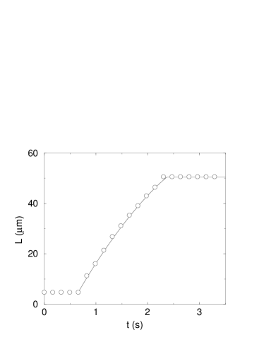
FIG. 2.: Progress of the leading edge of a SOPC/CHOL mixed lipid vesicle down the pipette (reproduced from figure 3 of [5]). For this event $R_{\rm init}=17.6\,\mu$m and $p=353$ dyn/cm². The initial velocity ($v_{\rm init}$) is approximately $35\,\mu$m/s. The solid line depicts the theoretical $L(t)$ curve for our stabilized pore model.

These two sources of friction control the speed of the vesicle front. As we will show in the following sections, they also determine the stable pore size and when and if the pore recloses so as to stop the inhalation process. As the projected length of membrane inside the micropipette grows, so does the amount of friction. We will identify a feedback mechanism through which the velocity, and hence the surface tension, becomes a function of the pore size. This modifies the effective energy function (Eq. 1) and in doing so, generates a second stable minimum at a finite pore radius ($r_{\rm stable}$). At $L_{\rm crit}$ the stable minimum disappears and the pore snaps shut.

III Stabilization Mechanism

The feedback mechanism mentioned above requires the surface tension on the exterior bulb to be a function of the projected length of membrane in the pipette and the pore size. The first step is to write this tension in terms of the pressure inside the bulb ($p_{\rm 2}$) using the Laplace formula:

$$p_{\rm 2}={{2\Sigma}\over{R}}\ .$$ (4)

Here $R$ is the radius of the bulb. This formula really only applies at equilibrium; fortunately the membrane’s fast relaxation and the fact that $R$ and $p_{\rm 2}$ change rather slowly imply that the surface is never far from this ideal.

The radius of the bulb $R$ is already a simple function of $L$. The necessary relation is obtained from the constraint of fixed vesicle area. We thus have an equation that determines the bulb radius as a function of projected length ($L$):

$$4\pi R^{\rm 2}+\pi d_{\rm v}L=4\pi R_{\rm init}^{\rm 2}\ .$$ (5)

Here $R_{\rm init}$ is the radius of the bulb at the time the pore is created while $d_{\rm v}\equiv d_{\rm p}-h$ gives the diameter of the cylindrical portion of the vesicle inside pipette. Eq. 5 assumes the bulb region remains spherical and that the area of the leading edge does not change significantly as $L$ increases.

The pressure inside the bulb must still be found in terms of $L$. This is achieved by considering the interface at the leading edge of the vesicle. Here we can apply Laplace’s formula again:

$$p_{\rm 1}+p_{\rm 2}={{4\Sigma_{\rm 0}}\over{d_{\rm v}}}\ .$$ (6)

Implicit in this equation is the assumption that the pressure is uniform everywhere inside the vesicle. There will in fact be a small pressure gradient near the pipette mouth due to convergent flow. This pressure change is on the order of $\eta v/d_{\rm v}$ and turns out to be negligible. Eqs. 4 and 6 can now be used to eliminate $p_{\rm 2}$. In addition, we can use Eq. 3 to remove $\Sigma_{\rm 0}$ and Eq. 2 to get rid of $p_{\rm 1}$. This gives us a new form for the surface tension:

$$\Sigma={{2R}\over{2R-d_{\rm v}}}\left({{{pd_{\rm v}}\over{4}}-\eta v\left({{{8(L_{\rm eff}-L)d_{\rm v}}\over{d_{\rm p}^{2}}}+{L\over h}}\right)}\right)\ .$$ (7)

This equation for the surface tension now has explicit dependence on the projected membrane length (both through $L$ itself and through the function $R(L)$). The dependence on the pore size enters only implicitly through the velocity.

The goal is now to find a suitable expression for the velocity to substitute into Eq. 7. Following [5], this can be achieved by considering the flow through the pore. As the vesicle moves into the pipette, its volume changes: solvent must exit through the open pore. We compute the rate of outflow ($Q$) in two different ways and compare to get $v$. The first way is to write $Q$ as the derivative of the total vesicle volume (Figure 1):

$$Q=-{\mskip 1.3mu{\rm d}\mskip 0.7mu\over{\mskip 1.3mu{\rm d}\mskip 0.7mut}}\left({{4\pi}\over 3}R^{\rm 3}+{{\pi d_{\rm v}^{\rm 2}L}\over 4}\right)={{\pi d_{\rm v}v}\over 4}(2R-d_{\rm v})\ .$$ (8)

Note that we have re-expressed all the time derivatives in terms of the velocity. The $R$ time derivative was obtained by differentiating the area constraint (Eq. 5):

$${{\mskip 1.3mu{\rm d}\mskip 0.7muR}\over{\mskip 1.3mu{\rm d}\mskip 0.7mut}}=-{{vd_{\rm v}}\over{8R}}\ .$$ (9)

The other expression for the outflow can be found from the pressure forcing the flow. Since the flow is at low Reynolds number, $Q$ is just proportional to the pressure drop across the pore [9]:

$$Q={{p_{\rm 2}r^{\rm 3}}\over{3\eta}}\ .$$ (10)

Eqs. 8 and 10 can now be combined with Eq. 4 to yield the desired expression for the velocity of the leading edge of the vesicle:

$$v={8\over{3\pi\eta d_{\rm v}}}{{\Sigma r^{\rm 3}}\over{R(2R-d_{\rm v})}}\ .$$ (11)

This equation can now be substituted back into Eq. 7 to yield the promised form of the surface tension. This form has the surface tension as a function of the projected length (L) and the pore size (r):

$$\Sigma(r,L)={{\alpha_{\rm 1}}\over{1+\alpha_{\rm 2}r^{\rm 3}}}\ ,$$ (12)

where

$$\alpha_{\rm 1} \equiv {{pd_{\rm v}}\over 4}{{2R}\over{2R-d_{\rm v}}}\ ,\quad\rm{and}$$ (13)

$$\alpha_{\rm 2} \equiv {{16}\over{3\pi(2R-{d_{\rm v})^{\rm 2}d_{\rm v}}}}\left({{{8(L_{\rm eff}-L)d_{\rm v}}\over{d_{\rm p}^{2}}}+{L\over h}}\right)\ .$$ (14)

These equations define the feedback mechanism through which the effective surface tension is modified by the friction terms outlined in the previous section. The next step is to see how this feedback mechanism accounts for the experimentally observed behavior — that is, to see how it stabilizes pores.

Our main physical hypothesis is now that at each moment the pore adjusts quickly to minimize an effective energy similar to Eq. 1, but with the tension replaced by the varying quantity just found (Eq. 12). As long as this effective energy has a nontrivial minimum, the pore size will track it. This gives the pore size, and hence $v\equiv\dot{L}$ via Eq. 11 in terms of $L$. We can then solve this ordinary differential equation to obtain the time course $L(t)$ and compare to the data in Figure 2. This program relies on the presence of two different time scales: a slow scale for changes of $L$ and $R$, and a much faster time scale on which the pore size $r$ adjusts and the membrane tension equilibrates. We are adiabatically eliminating the fast variable to obtain a simple dynamics for the slow one. Thus our effective pore energy depends on $L$:

$$E_{\rm eff}(r,L)=2\pi r\gamma-{{\pi\alpha_{\rm 1}r^{\rm 2}}\over{1+\alpha_{\rm 2}r^{\rm 3}}}\ .$$ (15)

This new form of the energy can indeed have two minima: the trivial one ($r=0$) that appeared before and a new one at a finite pore size, depending on $L$:

$$\left.{{\mskip 1.3mu{\rm d}\mskip 0.7muE_{\rm eff}}\over{\mskip 1.3mu{\rm d}\mskip 0.7mur}}\right|_{r_{\rm stable}} = 0$$ (16)

$$\rightarrow\gamma = {{\alpha_{\rm 1}r_{\rm stable}}\over{2}}{{2-\alpha_{\rm 2}r_{\rm stable}^{\rm 3}}\over{(1+\alpha_{\rm 2}r_{\rm stable}^{\rm 3})^{\rm 2}}}\ .$$ (17)

As long as $L$ does not exceed some critical value ($L_{\rm crit}$), there will be a pore size ($r_{\rm stable}(L)$) that satisfies this equation. When the projected length reaches this critical value, the second stable minimum disappears and the pore collapses (figure 3). At this point the second derivative of the energy must also vanish:

$$\left.{{\mskip 1.3mu{\rm d}\mskip 0.7mu^{\rm 2}E_{\rm eff}}\over{\mskip 1.3mu{\rm d}\mskip 0.7mur^{\rm 2}}}\right|_{r_{\rm stable,crit}} = 0$$ (18)

$$\rightarrow 0 = {{1-7(\alpha_{\rm 2}r_{\rm stable}^{\rm 3})_{\rm crit}+(\alpha_{\rm 2}r_{\rm stable}^{\rm 3})_{\rm crit}^{\rm 2}}\over{(1+(\alpha_{\rm 2}r_{\rm stable}^{\rm 3})_{\rm crit})^{\rm 3}}}\ .$$ (19)

The resulting equation is not an equation for the pore size, but rather for the product $\alpha_{\rm 2}r_{\rm stable}^{\rm 3}$, a pure number. The relevant root of equation (19) yields $(\alpha_{\rm 2}r_{\rm stable}^{\rm 3})_{\rm crit}\approx 0.146$. This number will be useful in the following section where we will use the critical condition to determine the three undetermined parameters in the problem: the effective pipette length ($L_{\rm eff}$), the thickness of the lubrication layer ($h$), and the line tension ($\gamma$) of the membrane.

FIG. 3.: Energy as a function of pore size for supercritical, critical, and subcritical lengths of aspirated membrane: $L=0,45.8,90\,\mu$m. ($L_{crit}=45.8\,\mu$m.)

As promised, we have succeeded in reducing the full dynamics of the problem to only one variable, the projected length ($L$). This can be seen by substituting the surface tension formulae (Eqs. 12 and 14) along with $R(L)$ (Eq. 5) and the newly determined pore size ($r_{\rm stable}(L)$) into the velocity (Eq. 11):

$$\dot{L}\equiv v(L) = {{8}\over{3\pi\eta}}\left({{\alpha_{\rm 1}(L)r_{\rm stable}(L)^{\rm 3}}\over{1+\alpha_{\rm 2}(L)r_{\rm stable}(L)^{\rm 3}}}\right)$$ (21)

$$\times{{1}\over{R(L)d_{\rm v}(2R(L)-d_{\rm v})}}\ .$$

This equation for $\dot{L}$ as a function of $L$ can now be integrated to obtain $L(t)$, then compared directly to the experimental results (figure 2).

IV Extraction of Parameters

In the last section we were able to find a stable pore size for each value of the projected length of membrane in the pipette. From this pore size we were then able to determine the velocity, Eq. 21. This equation is a first order nonlinear ordinary differential equation for $L$. The goal of this section is to fit the unknown parameters $\gamma$, $L_{\rm eff}$, and $h$ so that the solution $L(t)$ fits the event shown in figure 2. We will then use these values to explain the other SOPC/CHOL events documented in [5].

The model that we propose has seven parameters in all (table I). Of these, two are measured directly from microscope images, namely the initial bulb radius ($R_{\rm init}$) and the pipette diameter ($d_{\rm p}$). The pressure ($p$) at the manometer and the viscosity ($\eta$) of the solvent are also determined experimentally.

TABLE I.: Parameters in the Model Name Value $R_{\rm init}$, $p$ see table II $d_{p}$ $7.5\,\mu$m $\eta$ $0.014\,$erg s/cm³ $L_{\rm eff}$, $h$, $\gamma$ fixed by model

Of the remaining three parameters, Zhelev and Needham estimated $L_{\rm eff}$ and $h$ via auxiliary experiments, then deduced $\gamma$. As discussed in the second section, the effective pipette length was found using a rather different experiment and so in our analysis, it will be determined from the data. Our analysis will also yield a value for the lubrication thickness ($h$) that will be in good agreement with the experimental estimate of [5]. Finally we will deduce the last remaining parameter in the model: the line tension ($\gamma$).

[5] give the full time course for one event, which we will use to find the three undetermined parameters listed above. This event is reproduced in Figure 2 and appears as the fourth entry in table II below. From the experimental $L(t)$ curve we first extract the projected length $L_{\rm crit}={\df 45.8}\,\mu$m at pore closure, the initial velocity $v_{\rm init}={\df 35.5}\,\mu$m/s, and the final velocity $v_{\rm crit}={\df 15.7}\,\mu$m/s. We will now use these numbers to determine the three unknown parameters: the effective pipette length ($L_{\rm eff}$), the lubrication layer thickness ($h$), and the line tension ($\gamma$).

The first step is to require that the pore lose its stability at the observed critical point; the second stable minimum in the energy must therefore disappear at $L_{\rm crit}$. As noted in the last section, the minimum vanishes when Eqs. 17 and 19 are satisfied. To get the pore size just before closure ($r_{\rm stable,crit}$) we use Eq. 21 at the critical point and require that it reproduce the observed final velocity. Recalling Eqs. 14 we then obtain:

$$v_{\rm crit}={\left({{(\alpha_{\rm 2}r_{\rm stable}^{\rm 3})_{\rm crit}}\over{1+(\alpha_{\rm 2}r_{\rm stable}^{\rm 3})_{\rm crit}}}\right)}{{pd_{\rm p}^{2}}\over{4\eta L_{\rm tot}}}\ ,$$ (22)

where we have defined

$$L_{\rm tot}\equiv 8(L_{\rm eff}-L_{\rm crit})+{{d_{\rm p}^{2}L_{\rm crit}}\over{d_{\rm v}h}}\ .$$ (23)

Eq. 22 can be solved for $L_{\rm tot}$. Then from Eq. 14 and the value of $(\alpha_{\rm 2}r_{\rm stable}^{3})_{\rm crit}$, one obtains the critical pore size:

$$r_{\rm stable,crit}={\left({(\alpha_{\rm 2}r_{\rm stable}^{\rm 3})_{\rm crit}{{3\pi(2R-d_{\rm v})^{\rm 2}d_{\rm p}^{2}}\over{16L_{\rm tot}}}}\right)}^{1/3}$$ (24)

In Eqs. 14 and 24 the value of $R$ is to be taken from Eq. 5 with $L=L_{\rm crit}$. Using the critical pore size obtained above, we can now go back to Eq. 17 to obtain a numerical estimate for the product of the line tension and a yet to be determined multiplier:

$$\gamma{{d_{\rm p}}\over{d_{\rm v}}} = {{pd_{\rm p}R}\over{4}}{\left({{3\pi d_{\rm p}^{2}(\alpha_{\rm 2}r_{\rm stable}^{\rm 3})_{\rm crit}}\over{16(2R-d_{\rm p})L_{\rm tot}}}\right)}^{{1}\over{3}}$$ (26)

$$\times{{2-(\alpha_{\rm 2}r_{\rm stable}^{\rm 3})_{\rm crit}}\over{(1+(\alpha_{\rm 2}r_{\rm stable}^{\rm 3})_{\rm crit})^{2}}}.$$

On the right hand side we have made the approximation $(2R-d_{\rm v})^{1/3}\approx(2R-d_{\rm p})^{1/3}$ which is accurate to within a couple of percent.

The next step is to determine the parameters $L_{\rm eff}$ and $h$. So far we have found only one combination of these, namely the quantity $L_{\rm tot}$ introduced in Eq. 23. To separate out the two contributions to $L_{\rm tot}$ we now require that the initial velocity ($v_{\rm init}$) come out as observed. From the velocity formula (Eq. 11) evaluated at $L=0$, we can find the effective pipette length in terms of the initial pore size ($r_{\rm stable,init}$) and the initial velocity:

$$L_{\rm eff}(v_{\rm init},r_{\rm stable,init}) = {{pd_{\rm p}^{\rm 2}}\over{32\eta v_{\rm init}}}-{{3\pi(2R_{\rm init}-d_{\rm v})^{\rm 2}d_{\rm p}^{\rm 2}}\over{128r_{\rm stable,init}^{\rm 3}}}$$ (27)

$$\approx {{pd_{\rm p}^{\rm 2}}\over{32\eta v_{\rm init}}}-{{3\pi(2R_{\rm init}-d_{\rm p})^{\rm 2}d_{\rm p}^{\rm 2}}\over{128r_{\rm stable,init}^{\rm 3}}}.$$ (28)

This form for $L_{\rm eff}$ can then be substituted back into Eq. 17 to obtain a sextic equation for $r_{\rm stable,init}$ that can be solved numerically. The solution so obtained can be substituted back into Eq. LABEL:Leff to yield a numerical estimate of $L_{\rm eff}$. Finally the lubrication layer thickness ($h$) can be recovered using Eq. 23. The approximations considered in Eqs. 26 and LABEL:Leff can now be refined using this new value of $h$ through a bootstrapping method.

To finish, we recover the line tension from Eq. 26 by multiplying through by the factor $(1-h/d_{\rm p})$. Thus all three of the required parameters can be determined from the single aspiration event depicted in Figure 2: $\gamma=2.6\times 10^{\rm-6}\,$erg/cm, $L_{\rm eff}=313\,\mu$m, and $h=0.48\,\mu$m. This value of $h$ agrees with Zhelev and Needham’s estimate, while our $L_{\rm eff}$ differs considerably from theirs.

TABLE II.: Comparison of experimental [5] and theoretical (this paper) closure times for SOPC/CHOL vesicles. $R_{\rm init}(\mu{\rm m})$ $p$ ( dyn/cm²) $t_{\rm exp}({\rm s})$ $t_{\rm th}({\rm s})$ $Bilayers$ $18.3$ $399$ $-^{*}$ $2.9$ $1$ $28.1$ $310$ $2.6$ $3.3$ $1$ $14.3$ $331$ $-^{*}$ $-^{*}$ $1$ $17.6^{\ddagger}$ $353$ $1.7$ $1.7$ $2$ $17.0$ $324$ $0.33$ $0.31$ $2$ $16.3$ $337$ $0.33$ $0.47$ $2$ $16.0$ $355$ $2.0$ $1.0$ $2$ $25.6$ $168$ $11.0$ $11.0$ $1$ $22.5$ $240$ $5.5$ $5.5$ $1$ $16.2$ $320$ $2.5$ $4.6$ $1$ ^∗ Did not reseal ^‡ Event used to determine $L_{\rm eff}$, $h$, and $\gamma$

With the parameters so determined, it is now possible to determine the time evolution of the other events in [5] from the initial conditions. For each of the other nine SOPC/CHOL events reproduced in table II, we integrated Eq. 21 for the given initial bulb radius ($R_{\rm init}$) and pressure ($p$) to obtain the critical time at which the pore closed. In some cases a double-bilayer with twice the nominal line tension was needed to fit the data [5]. The table compares the experimental time to closure found by Zhelev and Needham to the theoretical time determined using the model. The same effective pipette length, lubrication thickness and line tension were used for all ten events. An effort to optimize the values of the three parameters ($L_{\rm eff}$, $\gamma$, and $h$) based on a least squares fit to the critical time data did not produce results significantly different from those presented above.

Although the parameters were fixed by data from a single event, they produce reasonable critical times for the entire data set. The first event in table II is clearly an exception which we have no explanation for. Perhaps there was a large fluctuation in the manometer pressure or perhaps the electric field generated a pore so large that relaxation to the stable pore size was impossible. Despite this anomaly we are confident that we have faithfully determined the line tension of the SOPC/CHOL membrane making up the vesicles in question.

V Conclusion

In this paper we have explained the existence of the large dynamically-stabilized pores observed by [5]. By separating the fast timescale on which the membrane relaxation occurs from the slow one associated with the motion of the aspirated vesicle down the pipette, we have been able to establish a modified pore energy function with a stable minimum in the one micron range. In addition, we have described a new mechanism by which this minimum disappears destabilizing the pore.

The theory that we have developed permits an accurate determination of an important membrane parameter: the line tension. From a single event in Zhelev and Needham’s work, we were able to determine this parameter and two auxiliary parameters. The values so determined were then used to reconstruct all ten of the published SOPC/CHOL mixed lipid events: our theoretical post-prediction for the critical time at which pore stability is lost agreed well with the experimental result for all but one event. The agreement supports the value of our theory as a method for experimentally determining the line tension of bilayer membranes.

Acknowledgements: We would like to thank R. Kamien, U. Seifert, and D. Zhelev for helpful discussions, and the referee for suggesting an improvement to our calculation. This work was supported in part by the US/Israeli Binational Foundation grant 94–00190 and NSF grant DMR95–07366. JDM was supported in part by an FCAR Graduate Fellowship from the government of Quebec.

REFERENCES

- [1] C. Taupin, M. Dvolaitzky, and C. Sauterey, Biochemistry 14, 4771 (1975).
- [2] W. Harbich and W. Helfrich, Z. Naturforsch. 34a, 1063 (1979).
- [3] L. Chernomordik et al., Biochim. Bioph. Acta 812, 643 (1985).
- [4] S. Leikin et al., J. Theor. Biol. 129, 411 (1987).
- [5] D. Zhelev and D. Needham, Biochimica et Biophysica Acta 1147, 89 (1993).
- [6] D. Zhelev and D. Needham, in Biological effects of electric and magnetic fields, edited by D. Carpenter and S. Ayrapetyan (Academic Press, San Diego, 1994), pp. 105–142.
- [7] E. Evans and W. Rawicz, Phys. Rev. Lett. 64, 2094 (1990).
- [8] D. Chang, B. Chassy, J. Saunders, and A. Sowers, Guide to electroporation and electrofusion (Academic Press, San Diego, 1992).
- [9] J. Happel and H. Brenner, Low Reynolds number hydrodynamics (Prentice-Hall, Englewood Cliffs, NJ, 1965).