Summing graphs for random band matrices

Abstract

A method of resummation of infinite series of perturbation theory diagrams is applied for studying the properties of random band matrices. The topological classification of Feynman diagrams, which was actively used in last years for matrix model regularization of $2d$-gravity, turns out to be very useful for band matrices. The critical behavior at the edge of spectrum and the asymptotics of energy level correlation function are considered. This correlation function together with the hypothesis about universality of spectral correlations allows to estimate easily the localization length for eigen-vectors. A smoothed two-point correlation function of local density of states $\overline{\rho(E_{1},i)\rho(E_{2},j)_{c}}$ as well as the energy level correlation for finite size band matrices are also found. As $d$-dimensional generalization of band matrices lattice Hamiltonians with long-range random hopping are considered as well.

I Introduction

Random band matrices were introduced many years ago by E.Wigner [1] as a model Hamiltonian for complicated quantum systems. In the last few years statistical properties of random band matrices have become again the subject of intensive analytical and numerical investigation [2, 3, 4] due to their application to condensed matter physics and statistics of spectrum of chaotic systems.

Up to now all the analytical results for this quasi-$1d$ systems (for review see [2]) were obtained by mapping them onto a super-symmetric $\sigma$-model [5]. However, in this paper we would like to develop another method for calculations with random banded matrix ensembles. Roughly speaking our method consists of summation of infinite series of perturbation theory diagrams. Diagrammatic methods were used many years ago [7, 6] for investigation of Gaussian ensembles of $N\times N$ matrices but later this approach was almost forgotten for years. Our aim in this paper will be to show how this “ancient” method may lead rather easily to new results for band matrices.

Let us consider a Gaussian ensemble of random band matrices. Due to the Wick theorem such ensembles may be completely defined by the second moment:

$$\overline{H_{ij}H_{kn}}=F(i-j)(\delta_{jk}\delta_{in}+\Theta\delta_{jn}\delta_{ik})\,\,.$$ (1)

The function $F(i-j)=F(|i-j|)$ vanishes very rapidly outside the band (at $|i-j|>b\gg 1$). Parameter $\Theta$ takes values $0$ or $1$. If $\Theta=0$, one is dealing with Hermitian matrices of general form (Gaussian unitary ensemble - GUE), while $\Theta=1$ corresponds to the real symmetric matrices (Gaussian orthogonal ensemble - GOE). It is convenient to define the width of the band $b$ and the typical strength of the interaction $V$ through moments of the function $F$:

$$b^{2}=\frac{F_{2}}{F_{0}}=\frac{\sum n^{2}F(n)}{\sum F(n)}$$ (2)

$$V^{2}=F_{0}=\sum F(n)\ \ \ .$$ (3)

For practical computations we will sometimes use $F$ of the form

$$F(i-j)=\frac{V^{2}}{b\sqrt{2\pi}}\exp\left(-\frac{(i-j)^{2}}{2b^{2}}\right)\,\,.$$ (4)

As will be shown below the results essentially do not depend on the details of the shape of function $F(i-j)$. We need only $F(i-j)$ to be sufficiently smooth so that after averaging (1) all discrete sums may be replaced by integrals up to negligible corrections $\sim\exp(-b)$. In doing so we still are able to consider the corrections of any finite order in $1/b$. Moreover, we argue below that even smoothness of $F$ does not seem to be necessary for most interesting applications (see (19,20) and discussion below, it will be shown also why (4) is the most natural choice of $F$).

By simple $d$-dimensional extension of band matrices one obtains the Hamiltonian for particle hopping on a $d$-dimensional lattice with random nonlocal interaction. This lattice model may be described by the same formulas (1-4) with simple replacement of all integer indices by the integer $d$-vectors and trivial redefinition of $F$

$$i\rightarrow\vec{i}\,\,\,,\,\,\,F(\vec{i}-\vec{j})=\frac{V^{2}}{b(2\pi)^{d/2}}\exp\left(-\frac{(\vec{i}-\vec{j})^{2}}{2b^{2/d}}\right)\,\,.$$ (5)

Contrary to band matrices, properties of this model seem to be completely unknown. The $b\gg 1$ in (5) is effectively the number of “neighbors”, connected to each lattice site. The band matrices (1) may be associated now with the random Hamiltonian for one dimensional lattice.

The “physical quantities” which we would like to consider are connected with the Green’s function and the local density of states

$$G_{{i},{j}}(E)=\left(\frac{1}{E-H}\right)_{{i},{j}}\,\,\,,\,\,\,\rho(E,{i})=\frac{1}{\pi}ImG_{{i},{i}}(E-i0)\,\,\,.$$ (6)

There is no summation over $i$ in $G_{i,i}$ in the last formula. More specifically we would like to consider the averaged density of states $\overline{\rho(E)}$ and the correlation of densities for different but very close energies (and even for different positions $i$ and $j$).

It is also constructive to compare our results with those for the ensembles of usual $N\times N$ random matrices, which are defined by the second moment

$$F(i-j)\equiv\frac{V^{2}}{N}\,\,\,;\,\,\,\overline{H_{ij}H_{mn}}=\frac{V^{2}}{N}(\delta_{jm}\delta_{in}+\Theta\delta_{jn}\delta_{im})\,\,.$$ (7)

This Hamiltonian may be considered as the $d=0$ reduction of the lattice model (5) . Historically three main approaches were applied for studying the statistics of the full $N\times N$ matrices. The description of this approaches may be found e.g. in papers [7, 8, 9]. The first one is summation of infinite power series in $V/E$ [7]. Another two methods are the replica trick [8] and the super-symmetry method [9].

The success of both replicas and super-symmetry is essentially based on the use of Hubbard–Stratonovich transformation. For $N\times N$ matrices this transformation reduces the problem to an almost trivial calculation of a few dimensional integral. On the other hand for band matrices even after Hubbard–Stratonovich one still is faced with a $\sigma$-model on one-dimensional lattice. Thus it seems quite probable that neither replicas, nor super-symmetry will lead to considerable progress in the lattice model (5).

The exact solution of $2d$ quantum gravity [10] stimulated the explosion of interest in matrix models. In this application of random matrices the discretized random surfaces appear as Feynman graphs in the perturbative expansion of the matrix integral. However, technically the famous double scaling solution of $2d$-gravity has nothing to do with summation of graphs. For ensembles invariant under orthogonal transformations it is useful to work with $N$ eigenvalues instead of all $N^{2}$ matrix elements. Unfortunately, for band matrices, or lattice hopping Hamiltonian we could not find such a simple solution, which is not based on the diagrammatic expansion. Nevertheless for models (1, 5) the topological classification of diagrams, which arose in $2d$-gravity (and originally in QCD [11]), simplifies drastically the summation of the series.

This experience of dealing with the matrix integrals for $2d$-gravity was later used for solving the problems typical for quantum chaos. In [12] a method of calculation of correlators of Green functions for ensembles of large $N\times N$ matrices was developed. An approach based on summation of perturbation theory series for various ensembles of random matrices was also used in the series of papers of Brezin and Zee (see e.g. [13] and the later papers of the same authors), though their diagrammatic technique differs from used in the present paper.

The statistics of band matrices with parameters of the band slowly varying along the diagonal was considered in [14]. The behavior of the edge of spectrum for this extensions of the model (1) showed some surprising similarities with the edge properties of matrix ensembles considered for the $2d$-gravity. The topological classification of the diagrams which we will explore below was also briefly discussed in [14].

The organization of this article is as follows. The general description of the diagrammatic technique is given in Section 2. By comparison with $N\times N$ case a diagrammatic proof of semicircle density of states is found. We also develop partial summation of infinite subseries of topologically trivial tree-type diagrams. In Section 3 the ideology of double scaling limit is used to study the edge of spectrum for random band matrices. The edge of spectrum for lattice model (5) is considered in Section 4. Surprisingly the critical behavior at the edge for lattices with random hopping coincides with the critical behavior of the string-theory inspired model considered in [16]. In Section 5 the two-point correlation function $\overline{\rho(E_{1})\rho(E_{2})_{c}}$ is calculated. More precisely we found the so called smoothed correlation function in the large $b$ limit and the first $\sim 1/b$ correction to it. Moreover together with the hypothesis about the universality of spectrum fluctuations [19] this correlation function allows to find the correct estimate of the localization length for the eigenfunctions of band matrix. This universality holds also for the $\sim 1/b$ correction to the correlation function, even though the $\sim 1/b$ correction itself turns out to be a subject of strong cancellations. Finally in the Section 6 some quantities which have no analog for usual $N\times N$ matrices are considered. These are the correlation function of local density states $\overline{\rho(E_{1},i)\rho(E_{2},j)}_{c}$ and the usual density-density correlation function for the banded matrices of finite size $N$.

II Diagrammatic technique

It follows immediately from (1), that only diagonal terms survive in the averaged Green function

$$\overline{G_{i,j}}=G(E)\delta_{i,j}\,\,\,.$$ (8)

Let us expand $G(E)$ in a formal series

$$G=\frac{1}{N}\overline{tr\frac{1}{E-H}}=\frac{1}{NE}\sum_{n=0}^{\infty}\overline{tr\left(\frac{H}{E}\right)^{n}}\,\,\,.$$ (9)

Now all we need is using the Wick theorem and the second moment (1) to calculate all the average values of the trace of product of $H$ - matrices. In the standard Feynman diagram technique each $H^{n}$ corresponds to $n$-legs vertex and the averaging in (9) reduces to counting of the number of possible ways of contracting these legs to each other. However, like in $2d$-gravity it is more convenient to draw the dual Feynman graphs. For dual diagrams each $H_{ij}$ corresponds to a segment with numbers $i$ and $j$ at the ends, while $H^{n}$ corresponds to $n$-vertex polygon with matrix indices $i_{1},i_{2},\dots i_{n}$ assigned to the vertices (see fig. 1a). It is also useful to draw the arrow on each segment showing the direction from first to second index. Within this language the Wick contractions in (9) correspond to the glueing of pairs of segments. Our aim now is to calculate the number of ways in which the edges of the polygon may be glued into some closed surface.

For Hermitian matrices ($\Theta=0$ in (1)) the segments should be glued in the opposite direction thus forming the oriented surface. For symmetric matrices ($\Theta=1$) the nonoriented surfaces are also allowed (e.g. the Möbius band).

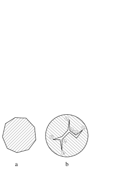
FIG. 1.: One plaquette a. and sphere b. glued from such plaquette

The example of simplest surface of spherical topology is shown in fig. 1.b. It is easy to verify that just the spherical surfaces dominate in $G$ at large $b$. Only in this case the sum over $n$ matrix indices for $H^{n}$ gives the factor $Nb^{0}$ and thus (see (1),(2))

$$G_{spherical}\sim b^{0}\,\,\,.$$ (10)

Moreover, as may be seen from fig. 1b, the summation over each index in spherical diagrams is completely independent and results in a fixed factor $V^{2}$ for any choice of the function $F(i-j)$ (4) and for each of ensembles (1),(5),(7). In particular this means (analogous observation was also done in [13]) that the Green function in the leading approximation coincides for all ensembles (1),(5),(7)

$$G_{0}=\frac{1}{2V^{2}}\bigl{(}E-\sqrt{E^{2}-4V^{2}}\bigr{)}$$ (11)

(a very clear proof of this formula for full $N\times N$ matrices see in [7, 6]).

Before considering the $\sim 1/b$ corrections let us carefully examine equation (11). As we have said above, $G_{0}$ may be thought as the exact sum of the part of the series (9) corresponding to diagrams of spherical topology. It is seen from (11) that this series is convergent only outside the circle on the complex $E$ plane with a radius $|E|=2V$. The values of $G_{0}$ inside the circle ($|E|<2V$) may be found via analytic continuation. This feature of the series has two important physical consequences. Firstly, if one is approaching the singular points $E=\pm 2V$ starting from large $E$ the more and more complicated diagrams became important thus approaching some kind of continuum limit. It may be not so obvious from the equation (11) because for $G_{0}$ the series converges even at $E\equiv\pm 2V$ but as we will see below the $\sim 1/b$ corrections to $G$ are more singular and the summation of $(V/E)^{n}$ do is saturated by the terms with very large $n$.

Even more troublesome turns out to be the calculation of correlation functions. In this case one has to consider the Green functions close to the borders of the cut ($E=E_{0}\pm i0\ ,\ |E|<2V$) and very far from the domain of convergency of the series(9). The price for such unreliable procedure will be the severe cancellations of different contributions to the $\sim 1/b$ corrections to correlation function (see Section 5).

As we have taken into account exactly in (11) all spherical contributions, the $\sim 1/b$ corrections naturally turn out to be determined by the diagrams of the more complicated topology. As we have seen before (10),(11) the sum over spherical graphs for full $N\times N$ matrices and for band matrices coincides up to trivial replacement $N\rightarrow b$ because the summation over each matrix index in the tree diagram of the kind of fig. 1b is independent and results exactly in the trivial factor $V^{2}$. This direct correspondence does not holds for the diagrams of the more complicated topology. However, each sum over matrix index contains effectively $\sim b$ items and their magnitude corresponds to that for $N\times N$ matrices up to substitution $b\rightarrow N$. Thus all the business with classification of the diagrams in the powers of the parameter $1/b\ (1/N)$ , which was so productive for the full matrices, still holds for the band matrices as well. In particular for the Hermitian band matrices ($\Theta=0$ in (1)) one may use the well known Eulers theorem to show that the corrections to (11) may be only of the kind $\sim(1/b^{2})^{n}$ with $n$ being the number of handles.

Up to now we have associated each Feynman diagram with some surface. However, as it may be seen e.g. from the fig. 1 because in our problem we have in fact one large plaquette (or two for the correlation functions) it is natural to consider only the border of this plaquette which should be glued to some kind of branched polymer. It is seen from the fig. 1b that the spherical surfaces are associated with the tree–type polymers. On the other hand the $\sim 1/b$ corrections to $G$ will be associated with selfintersections (the closed loops) of the polymer. It seems very attractive to divide the calculation of the $\sim 1/b$ corrections into two stages. The first stage will consists in summation over the trees and at the second stage one will take into account only the dressed selfintersected diagrams. To this end it turns out to be useful to consider instead of the Green function the logarithm

$$L(E)=\frac{1}{N}\overline{tr\ln\left(1-\frac{H}{E}\right)}\ \ ,\ \ G(E)=\frac{1}{E}+\frac{dL}{dE}\ .$$ (12)

The simple combinatorial calculation allows to replace the perturbative series for $L(E)$ by the sum over skeleton graphs, as it is demonstrated in the fig. 2

$$L(E)=-\frac{1}{N}\overline{\sum_{n=1}\frac{1}{n}tr\left(\frac{H}{E}\right)^{n}}=-\frac{1}{N}\overline{\sum_{\begin{array}[]{c}{\scriptstyle no\ contractions}\\ {\scriptstyle of\ neighbours}\end{array}}\frac{1}{p}tr\left(G_{0}H\right)^{p}}$$ (15)

Here the contractions between the nearest neighbours in the last sum are forbidden because they have been taken into account exactly in $G_{0}$-s. More precisely for the real symmetric matrices ($\Theta=1$ in (1)) the contractions between neighbours still are allowed but only due to the second term ($\sim\Theta$) in the r.h.s. of (1).

FIG. 2.: Reduction of $\overline{\ln(1-E/H)}$ to skeleton diagram.

III The edge of spectrum

Now at last we are able to consider the edge behavior of the $\sim 1/b$ corrections to the Green function $G_{0}$ (11). To this end in particular we have to take into account the long chains of glued dressed links of the kind of (15) (or fig. 2). Consider the simplest two-link chain which is shown in the fig. 3:

$$\Psi_{n}(i_{n}-i_{0}) = \sum_{i_{1}i_{2}\dots i_{n-1}}(\overline{H_{i_{0}i_{1}}H_{i_{1}i_{0}}})(\overline{H_{i_{1}i_{2}}H_{i_{2}i_{1}}})\dots(\overline{H_{i_{n-1}i_{n}}H_{i_{n}i_{n-1}}})$$ (16)

$$= V^{2n}\frac{1}{b\sqrt{2\pi n}}\exp\left\{-\frac{1}{2nb^{2}}(i_{0}-i_{n})^{2}\right\}\ \ .$$ (17)

Here in order to calculate $\Psi_{n}$ we have used the specific form of the function $F(i-j)$ (4). The various methods may be used in order to prove (16). For example one may use the mathematical induction method. While deriving the equation (16) we have replaced all the summations over the intermediate indices $i_{1},i_{2},\,...\,,i_{n-1}$ by the integrations. The accuracy of such procedure $\delta\Psi\sim e^{-b}$ for any smooth function $F(i-j)$ still allows one to consider the $\sim(1/b)^{n}$ corrections for any $n<b$ .

FIG. 3.: Double-line chain calculated in (13).

The $\Psi_{n}$ evidently satisfies the sum rule

$$\sum_{i_{n}}\Psi_{n}(i_{n}-i_{0})\equiv V^{2n}\ \ ,$$ (18)

which also may be used in order to find the normalization of (16).

The sum rule (18) holds exactly for any choice of the function $F(|i-j|)$ while the equation (16) is model dependent. However, as it will be shown now, for large $n$ the equation (16) is also universal. Consider the recursion formula for large $n$ (and arbitrary $F$)

$$\Psi_{n+1}(i)=\sum_{j}F(|i-j|)\Psi_{n}(j)=V^{2}\Psi_{n}(i)+\frac{V^{2}b^{2}}{2}\frac{d^{2}}{di^{2}}\Psi_{n}(i)+\,...\ \ \ .$$ (19)

This equation is the discrete (in time) analog of the heat conductivity equation. Together with the initial condition

$$\Psi_{0}(i)\sim\delta(i)\ \ ,$$ (20)

and the sum rule (18) equation (19) allows to reproduce the formula (16) for the chain. In fact this is the reason for considering the function $F(|i-j|)$ of the form (4) as the most universal one. Moreover, even if one starts with some irregular function $F$ (which may seem to be crucial because only for smooth $F(x)$ the summation may be replaced by integration with the accuracy $\sim e^{-b}$), taking into account of a long chains ($n\gg 1$) effectively smooth it out.

Up to now we have considered only the band matrices. However the formula (16) may be easily generalized for the random-bond lattice case (5)

$$\Psi_{n}(\vec{i}\,)=\frac{V^{2n}}{b(2\pi n)^{d/2}}\exp\left\{-\frac{1}{2nb^{2/d}}\vec{i}^{\,2}\right\}\ \ .$$ (21)

FIG. 4.: The Möbius band corresponding to the $\sim 1/b$ correction to Green function for real symmetric matrices.

At this point we have completed all the preliminary formalities and are able to calculate the $\sim 1/b$ correction to the Green function. Let us consider the ensemble of real symmetric matrices(GOE) for which the correction of the first order $\sim 1/b$ exists. The corresponding skeleton Feynman graph is shown in the fig. 4. It is seen from the figure that the collinear links should be glued in the $(1/b)^{1}$ order and thus this diagram is forbidden for the Hermitian(GUE) matrices. In terms of surfaces fig. 4 corresponds to the Möbius band. Combining together (12), (15) and (16) one finds the correction

$$L_{1}=\frac{1}{N}\overline{\delta\ln\left(1-\frac{H}{E}\right)}=-\frac{1}{N}\sum_{p=1}^{\infty}\frac{1}{2p}G_{0}^{2p}\,\overline{trH^{2p}}_{skeleton}=-\frac{1}{b}\sum_{p=1}^{\infty}\frac{1}{2p}(G_{0}V)^{2p}\frac{1}{(2\pi p)^{d/2}}\ ,$$ (22)

or for the Green function

$$G_{1}=\delta G=-\frac{1}{b(2\pi)^{d/2}}\frac{G_{0}^{\prime}}{G_{0}}\sum_{p=1}^{\infty}\frac{(G_{0}V)^{2p}}{p^{d/2}}\ \ .$$ (23)

We give the result at once for arbitrary dimensionality $0\leq d<\infty$. For band matrices one has to choose $d=1$.

The only important factor which is responsible for the difference between usual $N\times N$ matrices ($d=0$), band matrices and, random hopping Hamiltonians in (23) is the $1/p^{d/2}$ in the sum. Technically this factor comes from the double chain of matrix elements (16,21). One may consider the length of the Möbius band (fig. 4) $p$ as the discrete time in the diffusion equation (19). Then the $1/p^{d/2}$ will simply correspond to the time dependance of the return probability for classical diffusive particle at the time $p$ for different dimensions.

We are mostly interested in the singularities of $G$ at $G_{0}V\rightarrow 1$ (or $E\rightarrow\pm 2V$, see (11)). It is seen from (22) that $L_{1}$ has a finite limit at $G_{0}V=1$ for any $d>0$. On the other hand the $G_{1}$ (23) is convergent and the diagram of fig. 4 approaches the continuum limit, at least for $d=1$ and $d=2$ (for $d>2$ the $G_{1}$ is also singular, but mostly due to $G_{0}^{\prime}$ without any continuum limit).

For the random band matrix case ($d=1$) it is easy to found from (23), (11) that close to singular point

$$G(E\rightarrow 2V)=\frac{1}{V}-\frac{1}{V}\sqrt{\frac{E-2V}{V}}+\frac{1}{b}\,\frac{1}{4V}\left(\frac{V}{E-2V}\right)^{3/4}+\frac{1}{b^{2}}\frac{const}{V}\left(\frac{V}{E-2V}\right)^{2}+\,...\ \ .$$ (24)

Here the last term is the order of magnitude estimate of the $\sim 1/b^{2}$ contribution. The Feynman diagrams corresponding to this contribution are shown in the fig. 5 (the explicit calculation of one of them will be presented below).

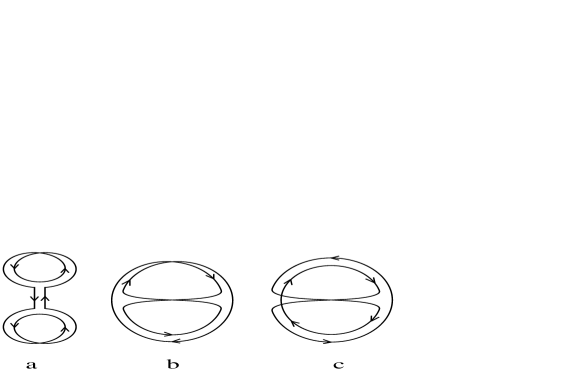
FIG. 5.: The three possible second order $\sim 1/b^{2}$ diagrams for ensemble of real symmetric (GOE) matrices, a. – dumb-bell shaped diagram, c. – torus

The simple counting of the power of convergency for the higher order diagrams shows that close to singularity the Green function should be described by some scaling function

$$G=\frac{1}{V}+\frac{1}{V}\frac{1}{b^{2/5}}\,\Phi\left(b^{4/5}\bigg{(}\frac{E-2V}{V}\bigg{)}\right)\ \ .$$ (25)

So, one may conclude that the singularity at the edge $E=\pm 2V$ of the perturbative Green function (11) should be smoothed out at the distances $\Delta E\sim Vb^{-4/5}$ from the singular points. For example it is easy to estimate the number of energy levels falling into this region. The same estimate evidently holds for the number of the levels outside the circle $|E|>2V$

$$\Delta N\sim N\Delta E^{3/2}\sim\frac{N}{b^{6/5}}\ \ .$$ (26)

This estimate is of particular interest because the density of eigenvalues outside of the circle is purely nonperturbative and could not be found in any finite order over $1/b$. It is to be noted that for usual $N\times N$ matrices (both GOE and GUE) $\Delta E\sim N^{-2/3}$ and $\Delta N\sim 1$.

As we have told in the introduction, random band matrix may be considered as a Hamiltonian for particle on $1d$ lattice with random hopping. Eigenvectors for such Hamiltonian should naturally have some finite localization length. This localization length for the band matrix ensembles (1) was found in the papers of Fyodorov and Mirlin [2] within the super-symmetry method (the calculation of $l_{loc}$ in our approach will be given in Section 5)

$$l_{loc}\sim b^{2}\left(1-\frac{E^{2}}{4V^{2}}\right)\ \ ,\ \ |E|<2V\ \ .$$ (27)

This result in fact was found only in the leading order in $1/b$ and should be changed at the edge of spectrum. One may combine our result (25) with (27) in order to estimate the localization length for nonperturbative states living outside of the main band (circle)

$$l_{loc}^{np}\sim b^{2}\Delta E\sim b^{6/5}\ \ .$$ (28)

In particular $l_{loc}^{np}\Delta N\sim N$ which may mean that nonperturbative states spatially do not overlap.

In the recent paper [15] the distribution of Lyapunov exponents for random band matrices was studied numerically at the very edge of perturbative part of spectrum $|E|=2V$. The authors of ref. [15] have considered the band matrices with step form of the band $F(|i-j|>b)\equiv 0$ for which there exist exactly $2b+1$ Lyapunov exponents. Their result reads

$$\lambda_{i}\sim b^{-4/3}i^{1/3}\ \ \ .$$ (29)

Here $i=1,2,3...$ , and $\lambda_{1}$ is the smallest decrement of the Lyapunov exponent. The corresponding solution grows like $\psi_{n}^{(i)}\sim\exp(n\lambda_{i})$. Naively one may expect that the smallest Lyapunov exponent directly gives the localization length

$$\lambda_{1}^{-1}\approx l_{loc}\ \ \ .$$ (30)

However, this simple guess puts in conflict the two results (28) and (29). On the other hand, the numerical accuracy of [15] allows one to be sure in (29) for sufficiently large $i$, namely $1\ll i\ll b$. The accurate result for smallest Lyapunov exponent still may differ from (29).

Moreover, the direct correspondence between the localization length and first Lyapunov exponent naturally take place in the central part of spectrum $|E|<2V$ but at the edge $|E|=2V$ formula (30) is not necessary correct. It seems rather probable that the eigenstates outside the circle $|E|\geq 2V$ appears due to some very rare fluctuations of our random banded Hamiltonian $H_{ij}$. Furthermore, we have no idea how even to estimate the density of such rare fluctuations. If the number of this fluctuations is small compared to $N/b^{6/5}$ the eigenstates with $|E|>2V$ will not be distributed homogeneously, but will be concentrated in rather rare and dense bunches. On the other hand, the first Lyapunov exponent $\lambda_{1}$ evidently comes from the whole range of variation of vector index. Thus the localization length at $|E|=2V$ should not be necessary of the same order of magnitude with the first Lyapunov exponent. Unfortunately, if the states with $|E|>2V$ do are concentrated together one should most naturally expect that $\lambda_{1}^{-1}\gg l_{loc}^{np}$. Thus, the discrepancy between (28) and (29) turns out to be even severe in this case.

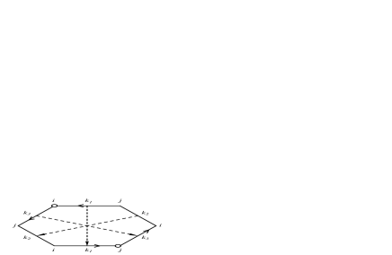
FIG. 6.: Gluening of dressed hexagon for $\sim 1/b^{2}$ correction for Hermitian matrices (torus).

In fact in (24), (25) the estimate for higher order corrections was declared without any proof. However, both for the more rigorous proof of (25) and for future calculations it is useful to calculate explicitly at least one nontrivial (beyond the one loop) diagram. Therefore we would like to found now the leading $\sim 1/b^{2}$ correction for the GUE band matrices. In this case the only diagram of fig. 5c survive which corresponds to torus in the surface language. The fig. 6 shows how one have to glue the dressed hexagon (see (15)) in order to built this diagram. Indices $k_{1},k_{2},k_{3}$ on the figure are the lengths of the double-link chains (16), while $i$ and $j$ stands for the matrix indices corresponding to the ends of these segments. It is to be noted that both indices $i$ and $j$ appear three times in the diagram, which in particular leads to loss of two powers of large $b$ for this diagram compared to the tree one (fig. 1b). More precisely, as it may be seen also from the diagram fig. 1b not the multiple indices but the closed loops are the direct source of the $1/b$ . One of the simplest ways to find the order of the diagram in the $(1/b)^{n}$ classification is to look for the number of links which are enough to break in order to get the tree-kind simply connected diagram. Now one may combine (15) and (16) in order to found the contribution of the fig. 5c

$$L_{2}^{H} = -\frac{1}{N}\sum_{k_{1},k_{2},k_{3}>0}\frac{1}{2(k_{1}+k_{2}+k_{3})}(k_{1}+k_{2}+k_{3})\frac{1}{3}(G_{0})^{2k_{1}+2k_{2}+2k_{3}}$$ (31)

$$\times \sum_{i,j}\Psi_{k_{1}}(i-j)\Psi_{k_{2}}(i-j)\Psi_{k_{3}}(i-j)\ \ .$$ (32)

Here $(k_{1}+k_{2}+k_{3})^{-1}$ comes from $1/p$ in (15) and the combinatorial factor $(k_{1}+k_{2}+k_{3})^{+1}$ takes into account the number of positions available, say, for the left end $i$ of the upper segment $k_{1}$ on the fig. 6 and the right end $j$ of the same down segment (these points are shown by the two small circles on the figure). Because these two circles $i$ and $j$ are equivalent the combinatorial factor is only $\sum k_{i}$ , not the $2\sum k_{i}$ . Finally, after one has taken into account by this $\sum k_{i}$ the freedom in definition of the starting point on the circle the sets $(k_{1},k_{2},k_{3})$, $(k_{2},k_{3},k_{1})$ and $(k_{3},k_{1},k_{2})$ became indistinguishable which is taken into account by the factor $1/3$ in (31). The simple substitution of (16) into (31) leads to

$$L_{2}^{H}=$$ (33)

$$-\frac{1}{6b^{2}}\sum_{k_{1},k_{2},k_{3}>0}\frac{(G_{0}V)^{2k_{1}+2k_{2}+2k_{3}}}{2\pi\sqrt{k_{1}k_{2}k_{3}}}\sum_{i}\frac{1}{b\sqrt{2\pi}}\exp\left\{-\frac{1}{2b^{2}}\bigg{(}\frac{1}{k_{1}}+\frac{1}{k_{2}}+\frac{1}{k_{3}}\bigg{)}(i-j)^{2}\right\}$$ (34)

$$\ \ \ =-\frac{1}{12\pi b^{2}}\sum_{k_{1},k_{2},k_{3}>0}\frac{(G_{0}V)^{2k_{1}+2k_{2}+2k_{3}}}{\sqrt{k_{1}k_{2}+k_{1}k_{3}+k_{2}k_{3}}}\ \ .$$ (35)

Thus the Green function close to the edge of spectrum for the GUE band matrices reads

$$G^{H} = \frac{1}{V}-\frac{1}{V}\sqrt{\frac{E-2V}{V}}+\frac{1}{b^{2}}\frac{I}{V}\left(\frac{V}{E-2V}\right)^{2}+\,...\,=$$ (36)

$$= \frac{1}{V}+\frac{1}{V}\frac{1}{b^{2/5}}\,\tilde{\Phi}\left(b^{4/5}\bigg{(}\frac{E-2V}{V}\bigg{)}\right)\ \ ,$$ (37)

where

$$I=\int_{x,y,z>0}\frac{\delta(1-x-y-z)}{48\pi}\frac{dxdydz}{\sqrt{xy+xz+yz}}\ \ .$$ (38)

In order to be sure that we have done nothing wrong with the combinatorics one may easily repeats the calculation (31-36) for usual $N\times N$ matrices. Some new (unknown) scaling function $\tilde{\Phi}$ appeared in (36). We have used the same argument for $\tilde{\Phi}$ as for $\Phi$ (25) but the asymptotic series for $\Phi(x)$ is in powers of $x^{-5/4}$ , while for $\tilde{\Phi}(x)$ in powers of $x^{-5/2}$ .

IV The edge of spectrum for lattices

Even more puzzling turns out to be the edge of spectrum behavior for the lattice ensembles (5). On the one hand, the naive power counting for diagrams like, e.g., the diagram of fig. 5c which we have calculated in (36) gives

$$G=\frac{1}{V}+\frac{1}{V}\frac{1}{b^{\frac{2}{6-d}}}\,\Psi\left(b^{\frac{4}{6-d}}\bigg{(}\frac{E-2V}{V}\bigg{)}\right)\ \ .$$ (39)

On the other hand, it is easy to find the first order ($\sim 1/b$) correction to the Green function at the edge from (23)

$$G_{1}=\frac{1}{8\pi bV}\sqrt{\frac{V}{E-2V}}\ln\left(\frac{V}{E-2V}\right)\ \ \ \ d=2\ \ \ ,$$ , (40)

$$G_{1}=\frac{1}{2bV}\sqrt{\frac{V}{E-2V}}\sum_{p=1}^{\infty}\frac{1}{(2\pi p)^{d/2}}\ \ \ \ d>2\ \ \ .$$ , (41)

It is seen immediately that at least for $d>2$ equations (40) and (39) disagree. In fact the solution to this paradox was found a few years ago in a paper of Ambjørn et al. [16] there the toy model for string in $d$-dimensions has been considered. The authors of ref. [16] have restricted the class of triangulations for string embedded in $d$-dimensions to those having minimal cross-section. While doing so they have obtained effectively the theory of $d$-dimensional branched polymer. As we have mentioned above, the summation over dual Feynman diagrams for our band matrices–lattices also reduces to summation over some branched polymers. In the lattice case indices assigned to the ends of each link expands over $d$-dimensional (although discretized) Euclidean space while the factor $F(\vec{i}-\vec{j})$ (5) regulates the spatial size of the link just like in the model of [16]. The branched polymers were also considered many times within the random vector–matrix models approach (see e.g. [17]). However, only the critical exponents for our model of branched polymers (or it is better to say “branched tapes” as it is seen from the figs. 4,5,7) should coincide with those for another models. The scaling function itself may be different.

FIG. 7.: Tadpoles or new trees for lattice models.

In order to solve the contradiction between (39) and (40) it is enough to observe that for $d\geq 2$ some of the diagrams for the branched polymer are much more singular than others with the same topology. These are the so called tadpole diagrams shown in fig. 7. Moreover, each of the diagrams of fig. 7 behaves effectively like some tree diagram (see fig. 1b) up to some trivial factor associated with the ends of the tree. Therefore, while the true complicated diagrams (say of fig. 5b,c) became less and less singular in higher dimensions in accordance with (39) the tadpole diagrams for $d>2$ have all the same singularity. On the other hand, one may try to sum up exactly this subseries of rather simple diagrams, as it was done in [16].

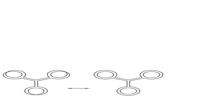
FIG. 8.: The reduction of tadpole diagram to corresponding correlation function.

The procedure of calculation of the tadpole contribution is illustrated by the fig. 8. Let us replace each $n$-tadpole diagram by some correlation function of our Green function and $(trH)^{n}$ calculated in the spherical approximation. Explicit formula corresponding to such procedure is as follows

$$G_{tadpole}=\frac{1}{N}\overline{\sum_{n}\left(tr\frac{1}{E-H}\frac{(\kappa\,trH)^{n}}{n!}\right)_{c}}\ \ \ ,$$ (42)

where subscript $c$ stands for connected diagrams. The coefficient $\kappa$ may be found for example from (40). The factor $1/n!$ in (42) accounts for the permutations of various $trH$. Due to this $1/n!$ the sum over $n$ results in the trivial exponentiation of $\kappa\,trH$. In order to find $G_{tadpole}$ it is useful to write explicitly the integration over $H$

$$G_{tadpole}=\frac{1}{Z}\int DH\frac{1}{N}tr\frac{1}{E-H}\exp\big{\{}-\sum_{i,j}H_{ij}H_{ji}M(i-j)+\kappa\,trH\big{\}}\ \ \ .$$ (43)

Here $M(i-j)\sim F(i-j)^{-1}$ and $Z$ is the same integral without $\frac{1}{N}tr\frac{1}{E-H}$ but with $\kappa\,trH$ included in the argument of the exponent. By such choice of $Z$ one gets rid of disconnected diagrams.

At least in the leading (spherical) approximation formulas (42) and (43) give the same Green function at the edge. On the other hand, the Green function (43) reduces to the zero order one (11) by trivial substitution

$$H_{ij} \rightarrow H_{ij}+const\,\delta_{ij}\ \ \ \ ,$$ (44)

$$E \rightarrow E+const\ \ \ \ .$$ (45)

After comparison with (40) one finds

$$G=\frac{1}{V}-\frac{1}{V}\sqrt{\frac{E-2V}{V}-\frac{1}{4\pi b}\ln\left(\frac{V}{E-2V}\right)}\ \ \ \ d=2\ \ \ ,$$ , (46)

$$G=\frac{1}{V}-\frac{1}{V}\sqrt{\frac{E-2V}{V}-\frac{1}{b}\sum_{p=1}^{\infty}\frac{1}{(2\pi p)^{d/2}}}\ \ \ \ d>2\ \ \ .$$ , (47)

For $d>2$ this result is almost trivial. Taking into account of the most singular series of corrections result in a simple shift of the edge of the cut. For $d=2$ taking into account of the tadpoles results not only in the shift of the edge by $\Delta E\sim\ln(b)/b$ but also in some nontrivial change of Green function. The singularity in (46) for $d=2$ will be smoothed out at $|E-2V-\frac{V}{2b}\ln(b)|\sim\frac{V}{b}$ by some unknown scaling function.

For GUE matrices(lattices) the simple tadpoles consisting of small Möbius band are forbidden. However one may arrange slightly more complicated $\sim 1/b^{2}$ tadpole shown on the fig. 9 which is allowed also for oriented surfaces. As a result for the GUE lattices with random bonds the critical dimension is $d=4$ instead of $d=2$.

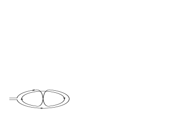
FIG. 9.: The $\sim 1/b^{2}$ tadpole for Hermitian(GUE) matrices.

V Correlation function

Physically may be the most interesting quantity which would be calculated with the random matrix ensembles is the two point correlation function of density of states at very close energies. It is generally believed that just such local quantities most adequately reproduce the measurable features of complicated quantum systems.

Unfortunately the perturbative procedure, which we are only able to perform, has a serious drawback in the case of correlation functions. As it was said in the Section 2, the perturbative series in $1/E$ are convergent only outside the circle $|E|>2V$ while the series in $1/b$ turns out to be the asymptotic series. Besides the perturbation theory there may exist some nonperturbative contributions say of the form $\sim\exp(-b(E-2V)^{\gamma})$ with some $\gamma\sim 1$ . However, after analytic continuation to the border of the cut, which goes from $E=-2V$ to $E=2V$ , these corrections may be (and do are at least for the usual $N\times N$ matrix ensembles) converted into some oscillating functions like $\sim\sin(b^{2}\Delta E)$ . Certainly in our perturbative result all these oscillating terms (if they are) will be smoothed out. For example for the usual GUE ensemble one gets instead of the exact result $K(\Delta E)=\sin^{2}(N\Delta E)/\Delta E^{2}$ only $K=0.5/\Delta E^{2}$ . Due to this principal limitation the quantities which we would calculate are called the smoothed correlators.

The intriguing feature of our diagrammatic series which was considered in the previous sections is that the dressed Feynman diagrams at the edge of spectrum approach some kind of continuum limit. Technically it happens because the value of $(VG_{0}(E))^{2}$ (11) which was our actual expansion parameter became equal to $(VG_{0}(2V))^{2}=1$ at the border. Now, because we are going to work with the energies inside the band $|E_{1,2}|<2V$ there seems to be no room for the continuum limit. However, let $E_{1}$ approach the upper border and $E_{2}$ approach the lower border of the cut . Then it follows immediately from (11) that

$$VG_{0}(E_{1}) = e^{i\phi-\lambda/2}\ \ \ ,$$ (48)

$$VG_{0}(E_{2}) = e^{-i\phi-\lambda/2}\ \ \ ,$$ (49)

where small $\lambda$ is given by

$$\lambda=\frac{E_{1}-E_{2}}{i\sqrt{4V^{2}-E^{2}}}\ \ \ ,\ \ \ Re\lambda > 0\ \ \ \ .$$ (50)

Thus again at least those subseries of diagrams which will have as the expansion parameter the combination $V^{2}G_{0}(E_{1})G_{0}(E_{2})=e^{-\lambda}$ may approach the continuum limit (another less direct example of the “effective” continuum limit will be considered in the following subsection).

In order to find the correlation function of two Green functions it is natural again to consider the logarithms

$$\overline{Tr\ln\left(1-\frac{H}{E_{1}}\right)Tr\ln\left(1-\frac{H}{E_{2}}\right)}_{c}\equiv$$ (51)

$$\equiv \sum_{p,p^{\prime}}\overline{\frac{1}{p^{\prime}}Tr\bigg{\{}(G_{0}(E_{1})H)^{p^{\prime}}\bigg{\}}_{skelet}\frac{1}{p}Tr\bigg{\{}(G_{0}(E_{2})H)^{p}\bigg{\}}_{skelet}}=$$ (52)

$$= 2\frac{N}{b(2\pi)^{d/2}}\sum_{p}\frac{p}{p^{2}}\frac{1}{p^{d/2}}\big{(}V^{2}G_{0}(E_{1})G_{0}(E_{2})\big{)}^{p}\ \ \ .$$ (53)

Here we have expanded each logarithm in the sum of closed skeleton chains like in eq. (15). Also here and below subscript $c$ means “connected”. A factor $2$ in front of the last sum accounts for two allowed directions of glued chains (Cooperon and diffuson in solid state physics). Finally, one combinatorial factor $p$ in the last sum accounts for the number of different ways to contract two skeleton rings of the length $p$. We see that just the $e^{-\lambda}$ (50) turns out to be the expansion parameter in (51).

By simple differentiation of (51) one finds the correlation function at very close energies $E_{1}-E_{2}\rightarrow 0$

$$\overline{Tr\frac{1}{E_{1}-H}Tr\frac{1}{E_{2}-H}}_{c} = \frac{2N}{b(4V^{2}-E^{2})}\sum_{p=1}^{\infty}\frac{p^{1-d/2}}{(2\pi)^{d/2}}e^{-\lambda p}\sim$$ (54)

$$\sim \left\{\begin{array}[]{ll}\left(\frac{i}{E_{1}-E_{2}}\right)^{2-d/2}\ \ ;\ \ d<4\\ \\ \ln\left(\frac{iV}{E_{1}-E_{2}}\right)\ \ ;\ \ d=4\end{array}\right.\ \ .$$ (58)

This equation reproduces the known result of Al’tshuler and Shklovskii [18] for correlation of energy levels in small disordered metallic samples.

The factor $1/p^{d/2}$ in (51,54) appears after glueing of two $H^{p}$ into closed two-link chain (16,21). As it was said also after eq. (23) this factor $1/p^{d/2}$ works effectively as the probability for diffusive particle to return to origin after time $p$. In principle one may go even further in this analogy with classical diffusion. By making the Fourier transform of the function $\Psi_{n}(\vec{i}-\vec{j})$ (16,21) the equation (54) may be written in the form of the integral of squared Green function of the diffusion equation (again in agreement with corresponding formulas from [18]).

Now let us consider in more details the correlation function for band matrices $(d=1)$. We would like to show how the information contained in the smoothed correlation function (54) combined with the simple hypothesis of universality of spectral correlations allows to find the correct estimate of the localization length for eigen-vectors of random band matrices. Consider instead of Green function $G$ the density of eigen-values $\rho(E)$ , which is simply the imaginary part of $G$ (6). It is generally recognized, that the fluctuations of $\rho(E)$ for all ensembles of full random $N\times N$ matrices are universal. This means that, being properly normalized, the density of states – density of states correlation function has the form:

$$\frac{\overline{\rho(E_{1})\rho(E_{2})_{c}}}{\overline{\rho(E_{1})}\ \overline{\rho(E_{2})}}=K\left(\frac{dn}{dE}(E_{1}-E_{2})\right)\ \ \ \ .$$ (59)

Here the function $K(x)\sim 1$ at $x\sim 1$ and $dn/dE$ is the averaged density of eigenstates. Of course, both $E_{1}$ and $E_{2}$ in (59) are real (have reached the border of the cut). The detailed form of $K(x)$ is specific for the ensemble under consideration (e.g. GUE or GOE), but for given ensemble $K$ is the universal function of energy interval $\Delta E=E_{1}-E_{2}$ measured in units of mean inter-level spacing $dE/dN$ .

For the random band matrices one may expect the same universal behavior of the correlation of density of state fluctuations as (59) only if all eigen-vectors are delocalized. On the other hand it is easy to write down the natural extension of the formula (59) for systems with finite localization length $l$ :

$$\frac{\overline{\rho(E_{1})\rho(E_{2})_{c}}}{\overline{\rho(E_{1})}\ \overline{\rho(E_{2})}}=\frac{l}{N}K\left(\frac{l}{N}\frac{dn}{dE}(E_{1}-E_{2})\right)\ \ \ \ .$$ (60)

By writing this formula we suppose that the fluctuations of density of energy levels for random band matrices still are universal if the energy difference $\Delta E=E_{1}-E_{2}$ is measured in the units of effective mean inter-level spacing

$$\Delta E_{eff}\sim\frac{N}{l}\frac{dE}{dn}\ \ \ \ .$$ (61)

Roughly speaking $\Delta E_{eff}$ is the mean inter-level spacing for a band matrix of a finite size $N\sim l$ (of course in (59,60) we suppose that at least $l\gg b$ ). Moreover, if the modified universality do takes place and $l\gg b$ the formulas (60,61) will also account for the energy dependence of the localization length. Of course the two universal functions $K(x)$ in (59) and (60) are completely different.

Our line of reasoning in fact follows the consideration of [19] (see also [20]) for density-density correlator in disordered metal. Now we would like simply to convert the arguments of authors of ref. [19] in order to estimate the localization length. The averaged density of states for large $b$ may be easily found from (11)

$$\overline{\rho(E)}=\frac{dN}{dE}=\frac{1}{\pi}Im\,\overline{trG(E-i0)}=\frac{N}{2\pi V^{2}}\sqrt{4V^{2}-E^{2}}\ \ .$$ (62)

Now from (54) one finds the asymptotics

$$\frac{\overline{\rho(E_{1})\rho(E_{2})_{c}}}{\overline{\rho(E_{1})}\ \overline{\rho(E_{2})}}=\frac{-1}{Nb}\ \frac{V^{4}}{(4V^{2}-E^{2})^{5/4}}\ \frac{1}{|E_{1}-E_{2}|^{3/2}}\ \ \ .$$ (63)

Together with (59) and (60) this correlation function allows to find:

$$l=\ b^{2}\left(1-\frac{E^{2}}{4V^{2}}\right)$$ (64)

in accordance with the result of Fyodorov and Mirlin [2]. We have defined here the localization length (or effective localization length) by choosing the overall normalization constant in (64) to be equal to one. Formally, universality–based arguments allows to find $l$ only up to some normalization constant $\sim 1$ , which on the other hand, depends on the explicit definition one uses for the localization length. For example, $l$ defined via the inverse participation ratio [2] or by the first Lyapunov exponent may differ by some trivial factor. Anyway, our estimate $l(E)$ seems to be much less complicated than those of the supersymmetric approach of [2].

A Corrections to the correlator

In this subsection we would like to consider the $\sim 1/b$ corrections to the correlation function. As it was explained above, we are able to calculate only the smoothed correlation functions. More concretely we are able to consider the Green functions not too close to the border of the cut $|ImE|\gg\Delta E_{eff}\sim V/b^{2}$ (61,64). Nevertheless, the uncertainty in the correlation function due to smoothening of fast oscillations decrease exponentially like $\sim\exp(-ImE/\Delta E_{eff})$. Therefore even for smoothed correlation function one is able to consider the corrections of any finite order in $1/b$.

The skeleton diagrams for $\sim 1/b$ correction to the correlation function (54,63) are shown in the fig. 10. At a first stage one may easily estimate the power of singularity for each diagram at small $\Delta E$. This singularities are associated with the number of summations over the length of tape glued from the segments originated from two different logarithms (51) $\ \ln(1-H/E_{1})$ and $\ \ln(1-H/E_{2})$. Thus compared to the zeroth order result (54,63) the diagrams of fig. 10a. are of the relative amplitude $\sim b^{-1}\Delta E^{-2+d/2}$ while the diagrams 10b. are of the relative amplitude $\sim b^{-1}\Delta E^{-1}$ .

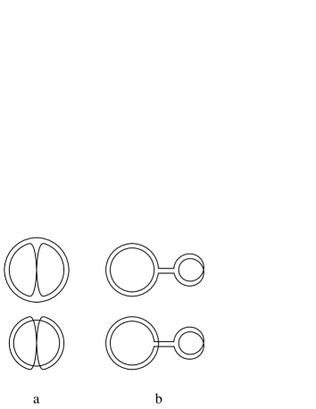
FIG. 10.: The $\sim 1/b$ corrections to correlation function. a. corrections singular like $1/\Delta E^{3}$ for $d=1$, b. corrections singular like $1/\Delta E^{5/2}$ for $d=1$.

On the other hand, the hypothesis of universality (60) which allows us to find so successfully the localization length (64) leads to a strong restriction on a possible form of corrections to the correlation function. As we have considered in the Section 2, the spherical result for the correlation function (63) is the exact result in the large $b$ limit. Therefore the corrections to (63) should be of the relative order $\sim 1/b$. In its turn due to the universality (60) $b$ may appear in the result only in the combination $(E_{1}-E_{2})/\Delta E_{eff}\sim(E_{1}-E_{2})l\sim(E_{1}-E_{2})b^{2}$ (see (60,61,64)). Thus the only form of the correlation function consistent with the universality condition (60) is

$$\overline{Tr\frac{1}{E_{1}-H}Tr\frac{1}{E_{2}-H}}_{c}\sim\frac{N}{b(E_{1}-E_{2})^{3/2}}\left(1+\frac{const}{b\sqrt{E_{1}-E_{2}}}+...\right)\ \ \ .$$ (65)

However, this expression evidently contradicts to the simple estimate of any of the diagrams of fig. 10.

Thus, we have to choose between the two scenarios. First, as it is seen from the naive estimates the $\sim 1/b$ corrections to the correlation function may be much more singular than it is expected from the universality (65). In this case the $\sim 1/b$ contributions blow up at $\Delta E$ much larger than the effective energy level spacing $\Delta E_{eff}$ (61) which will be the indication of some new physics at the intermediate energies $\Delta E_{eff}\ll\Delta E\ll V$ .

In the second scenario the universality (60,65) do takes place and all the additional singularities cancel each other in the sum of different diagrams.

In fact the aim of this section is to demonstrate explicitly that at least the $\sim 1/b$ corrections to the correlation function do not violate the universality (60,65) and all the additional singularities vanish after a huge cancellation between the diagrams of fig. 10.

The analogous cancellation between the high order corrections to the correlation functions has been previously observed for usual $N\times N$ random matrices by J.Verbaarschot et al. [7, 8].

Consider first the most singular diagrams of fig. 10a. The calculation of the corresponding contribution to the correlation function of two logarithms (51) has much in common with the calculation of the $\sim 1/b^{2}$ correction to the Green function at the edge (31-36). The main difference is that now two of the double-link chains are accompanied by the factor $(V^{2}G_{0}(E_{1})G_{0}(E_{2}))^{p}=e^{-\lambda p}$ , while the third chain is associated with the oscillating contribution $(V^{2}G_{0}^{2}(E_{1,2}))^{k}=\exp(\pm 2ik\phi-k\lambda)$ . It is convenient to brought together into one expression the both diagrams of fig. 10a

$$\delta\big{(}\overline{LL}\big{)}_{a} = \frac{2N}{b^{2}}\frac{1}{2}\sum_{p_{1},p_{2}>0}\,\sum_{-\infty<k<\infty}\frac{e^{2i\phi k-\lambda(p_{1}+p_{2}+|k|)}}{(2\pi)^{d}(p_{1}p_{2}|k|)^{d/2}}\left(\frac{1}{p_{1}}+\frac{1}{p_{2}}+\frac{1}{|k|}\right)^{-d/2}=$$ (66)

$$= \frac{N}{b^{2}}\sum\frac{e^{2i\phi k-\lambda(p_{1}+p_{2}+|k|)}}{(2\pi)^{d}(p_{1}p_{2}+|k|(p_{1}+p_{2}))^{d/2}}\ \ \ \ .$$ (67)

Naively summation over $p_{1}$ and $p_{2}$ here gives the singularity $\sim\lambda^{-2+d}$ (and the additional factor $\lambda^{-2}$ will appear after differentiation with respect to $E_{1}$ and $E_{2}$ which should be done in order to get the correlation function of two Green functions). However, at least this leading singularity should disappear after summation over $k$. For example, for $d=0$ one has $\sum_{k}e^{2i\phi k-\lambda|k|}\sim\lambda$ (even more trivial example of the same kind is $\sum(-1)^{k}=0$). For $d\neq 0$ some cancellation also should take place at least for large $p_{1,2}$ which, on the other hand, are responsible for the “naive” singularity of (66). Thus again one may see that large $k$ or long chains on the diagram (continuum limit) turn out to be important.

In order to treat this cancellation explicitly it is convenient to divide the contribution of fig. 10a into two parts

$$\delta\big{(}\overline{LL}\big{)}_{a} = A+B\ \ \ \ \ ,$$ (68)

$$A = \frac{N}{b^{2}(2\pi)^{d}}\sum_{p_{1},p_{2}>0}\,\sum_{-\infty<k<\infty}e^{2i\phi k-\lambda(p_{1}+p_{2}+|k|)}\left\{\frac{1}{(p_{1}p_{2}+|k|(p_{1}+p_{2}))^{d/2}}-\right.$$ (69)

$$- \left.\frac{1}{p_{1}^{d/2}(p_{2}+|k|)^{d/2}}-\frac{1}{p_{2}^{d/2}(p_{1}+|k|)^{d/2}}\right\}\ \ \ \ ,$$ (70)

$$B = \frac{2N}{b^{2}(2\pi)^{d}}\left[\sum_{p>0}\frac{e^{-\lambda p}}{p^{d/2}}\right]\sum_{p^{\prime}>0}\,\sum_{-\infty<k<\infty}\frac{e^{2i\phi k-\lambda(p^{\prime}+|k|)}}{(p^{\prime}+|k|)^{d/2}}\ \ \ .$$ (71)

Here in the part $A$ the contribution with large both $p_{1}$ and $p_{2}$ will be suppressed due to summation over $k$, while the contribution with say $p_{1}\ll p_{2}$ will be suppressed due to simple cancellation of the two terms in the figure brackets in (68). In the second part $B$ summations over $p$-s are factorized and only summation over $p^{\prime}$ suffers from the cancellation due to oscillations.

In the similar way one may write down the contribution of naively less singular diagrams of fig. 10b

$$\delta\big{(}\overline{LL}\big{)}_{b} = \frac{2N}{b^{2}(2\pi)^{d}}\left[\sum_{p>0}\frac{e^{-\lambda p}}{p^{d/2}}\right]\left\{\sum_{k\geq 0}e^{(2i\phi-\lambda)k}\sum_{q>0}\frac{e^{(2i\phi-\lambda)q}}{q^{d/2}}+(\phi\rightarrow-\phi)\right\}=$$ (72)

$$= \frac{2N}{b^{2}(2\pi)^{d}}\left[\sum_{p>0}\frac{e^{-\lambda p}}{p^{d/2}}\right]\left\{\sum_{-\infty<k<\infty}\,\sum_{-|k|<p^{\prime}\leq 0}\frac{e^{2i\phi k-\lambda|k|}}{(p^{\prime}+|k|)^{d/2}}\right\}\ \ \ .$$ (73)

The situation is further simplified if one combines this contribution with the most singular part $B$ (68) of the fig. 10a diagrams. After simple change of variables $p^{\prime}\rightarrow q=p^{\prime}+|k|$ one gets

$$\delta\big{(}\overline{LL}\big{)}_{b}+B = \frac{2N}{b^{2}(2\pi)^{d}}\left[\sum_{p>0}\frac{e^{-\lambda p}}{p^{d/2}}\right]\times$$ (74)

$$\sum_{-\infty<k<\infty}\,\sum_{q>0}e^{2i\phi k-\lambda|k|}\frac{1}{q^{d/2}}\exp\{-\lambda(q-|k|)\theta(q-|k|)\}\ \ \ .$$ (75)

Here $\theta(x)=0$ for $x<0$ and $\theta(x)=1$ for $x>0$. Now the sum over $k$ may be found exactly

$$\delta\big{(}\overline{LL}\big{)}_{b}+B=\frac{2N}{b^{2}(2\pi)^{d}}\left[\sum_{p>0}\frac{e^{-\lambda p}}{p^{d/2}}\right]\lambda\,\sum_{q>0}\frac{\cos(2q\phi)e^{-\lambda q}}{q^{d/2}2\sin^{2}\phi}\ \ .$$ (76)

We see that this contribution as a function of $\lambda$ turns out to be as singular as the leading order result (51,54) but is suppressed like $1/b$ and therefore should be neglected.

Thus, let us consider the only surviving contribution $A$ from (68). For simplicity consider the band matrices only ($d=1$). After differentiation with respect to $E_{1}$ and $E_{2}$ one gets

$$\delta(\overline{TrG_{1}TrG_{2}}) = \frac{N}{b^{2}2\pi(4V^{2}-E^{2})}\sum e^{2i\phi k-\lambda(p_{1}+p_{2}+|k|)}(p_{1}+p_{2}+|k|)^{2}$$ (77)

$$\times \left\{\frac{1}{\sqrt{p_{1}p_{2}+|k|(p_{1}+p_{2})}}-\frac{1}{\sqrt{p_{1}(p_{2}+|k|)}}-\frac{1}{\sqrt{p_{2}(p_{1}+|k|)}}\right\}\ \ \ .$$ (78)

As we will see both $p_{1}$ and $p_{2}$ in this sum effectively turns out to be large. Therefore, in order not to get exponentially small result one has to consider the singular in $k$ contributions in the sum. These singularities naturally appear due to $|k|$ in (77). The following simple identity shows how one may utilize this $\sim|k|$ behavior:

$$\sum|k|e^{2i\phi k-\lambda|k|}=\sum|k|e^{2i\phi k-\lambda|k|}f(k)=\frac{-1}{2\sin^{2}\phi}\ \ \ ,$$ (79)

where $f(k)$ is any smooth and slow function of $k$ and $f(0)=1$. Taking into account that $2V\sin\phi=\sqrt{4V^{2}-E^{2}}$ one finds from (77,79)

$$\delta(\overline{TrG_{1}TrG_{2}})=\frac{4NV^{2}}{b^{2}(4V^{2}-E^{2})^{2}}\sum_{p_{1},p_{2}}\frac{p_{1}+p_{2}}{2\pi\sqrt{p_{1}p_{2}}}e^{-(p_{1}+p_{2})\lambda}=\frac{-N}{b^{2}}\frac{2V^{2}}{4V^{2}-E^{2}}\frac{1}{\Delta E^{2}}\ \ .$$ (80)

Finally, the smoothed density-density correlation function for band matrices takes the form

$$K(E_{1}-E_{2})=\frac{N}{l}\frac{\overline{\rho(E_{1})\rho(E_{2})_{c}}}{\overline{\rho(E_{1})}\ \overline{\rho(E_{2})}}=\frac{-1}{2}\left(\frac{\Delta E_{eff}}{|E_{1}-E_{2}|}\right)^{3/2}\left\{1+2\left(\frac{\Delta E_{eff}}{|E_{1}-E_{2}|}\right)^{1/2}+...\right\}\ \ \ ,$$ (81)

where $\Delta E_{eff}=N[2\pi l\overline{\rho(E)}]^{-1}$ and $l=b^{2}(1-E^{2}/4V^{2})$ in accordance with (60,64,65). For convenience we have added one factor $(2\pi)^{-1}$ into the definition of $\Delta E_{eff}$ compared to (61).

To conclude this section let us remind again that we consider only the smoothed correlation functions. If one would like to compare our equation (81) with the result of numerical matrix diagonalization, the “experimental” result should be averaged with some smooth weight function. For example it may be

$$K_{smooth}(\Delta E)=\int K_{exp}(\Delta E+\kappa x)e^{-x^{2}}\frac{dx}{\sqrt{\pi}}\ \ \ ,$$ (82)

where $\Delta E_{eff}\ll\kappa\ll\Delta E$.

VI Spatially nonhomogeneous examples

The quantities which we have tried to calculate up to now – the density of states and density-density correlation function are generally considered for the usual $N\times N$ random matrices. In this section we would like to consider the two quantities which are specific for band matrices and never appear for the usual $N\times N$ ones.

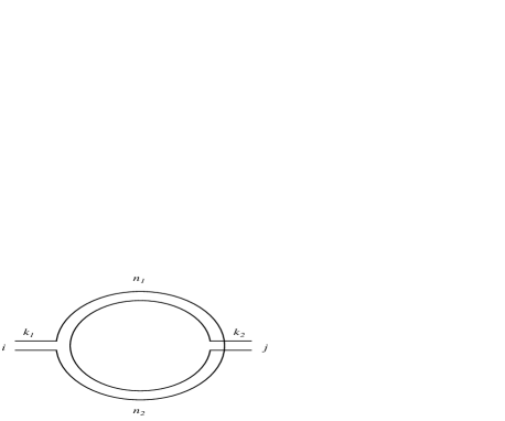
FIG. 11.: Spatially nonhomogeneous correlation function $\overline{\rho(E_{1},i)\rho(E_{2},j)}$.

The first example will be the correlation function of local density of states $\rho(E,i)$ for different energies and different vector indices ($1d$-lattice sites) $i$ and $j$. The corresponding dressed Feynman diagram is shown in the fig. 11. Again one should calculate first the log–log correlation function. After differentiation with respect to $E_{1}$ and $E_{2}$ and taking the imaginary part of the Green functions the correlation function takes the form

$$\overline{\rho(E_{1},i)\rho(E_{2},j)_{c}}=\frac{1}{\pi^{2}b^{2}}G_{0}(E_{1})G_{0}(E_{2})$$ (83)

$$Re\sum_{k_{1,2}\geq 0}\sum_{n_{1}+n_{2}>0}\frac{(G_{0}(E_{1})V)^{2k_{1}}(G_{0}(E_{2})V)^{2k_{2}}(G_{0}(E_{1})G_{0}(E_{2})V^{2})^{n_{1}+n_{2}}}{\sqrt{(k_{1}+k_{2})(n_{1}+n_{2})+n_{1}n_{2}}}$$ (84)

$$\ \ \ \ \frac{1}{2\pi}\exp\left\{-\frac{1}{2b^{2}}\frac{(i-j)^{2}}{k_{1}+k_{2}+\frac{n_{1}n_{2}}{n_{1}+n_{2}}}\right\}\ \ \ .$$ (85)

Here neither $n_{1}$ nor $n_{2}$ could be negative. This equation is further simplified if one takes into account that effectively $k_{1,2}\ll n_{1,2}$. Therefore the $k_{1,2}$ may be neglected in the exponent and in the square root in the denominator and the sum over $k_{1}$ and $k_{2}$ reduces to the simple geometrical progression. Finally, the summations over $n_{1}$ and $n_{2}$ factorize and the correlation function takes rather simple form

$$\overline{\rho(E_{1},i)\rho(E_{2},j)_{c}}=\frac{1}{\pi^{2}b^{2}(4V^{2}-E^{2})}Re\ \left[\sum_{n}\frac{e^{-\lambda n}}{\sqrt{2\pi n}}\exp\left\{-\frac{(i-j)^{2}}{2nb^{2}}\right\}\right]^{2}\ \ \ .$$ (86)

Here $\lambda$ is defined by (50). One may easily investigate for example small and large $i-j$ limits of this expression. In terms of universal variables $\Delta E_{eff}$ and $l$ (81) correlation function (86) takes the form

$$\frac{\overline{\rho(E_{1},i)\rho(E_{2},j)_{c}}}{(\overline{\rho(E)}/N)^{2}} = \frac{1}{2\pi}\left(\frac{i-j}{l}\right)^{2}\times$$ (88)

$$Re\ \left[\int_{0}^{\infty}\exp\left\{-\frac{1}{4i}\frac{E_{1}-E_{2}}{\Delta E_{eff}}\left(\frac{i-j}{l}\right)^{2}y^{2}-\frac{1}{2y^{2}}\right\}dy\right]^{2}\ .$$

Here $Im(E_{1}-E_{2})>0$ and the integral should be squared before taking the real part. We have divided $\overline{\rho(E)}$ by $N$ in the left hand side of (88) in order to get rid of the physically trivial $N$-dependance in the right hand side also.

Finally, the integration over $y$ in (88) may be done explicitly, which leads to

$$\frac{\overline{\rho(E_{1},i)\rho(E_{2},j)_{c}}}{(\overline{\rho(E)}/N)^{2}} = \frac{1}{2}Re\left[\frac{i\Delta E_{eff}}{E_{1}-E_{2}}\exp\left\{-\sqrt{2\frac{E_{1}-E_{2}}{i\Delta E_{eff}}}\frac{|i-j|}{l}\right\}\right]=$$ (89)

$$= -\frac{1}{2}\left(\frac{i-j}{l}\right)^{2}\frac{sin(t)e^{-t}}{t^{2}}\ \ \ ,$$ (90)

where $t={|i-j|}/{l}\sqrt{{|E_{1}-E_{2}|}/{\Delta E_{eff}}}$ . In particular one may easily examine that after summation over $i$ and $j$ the equation (89) leads to the usual correlation function (63).

Another interesting objects which may be considered easily within our technic are the finite size band matrices. Naturally the most interesting case is $b\ll N\leq b^{2}$. Below we describe analytically the crossover from the band matrix regime (54) to Wigner-Dyson regime in the asymptotics of smoothed density-density correlation function for finite size band matrices.

Consider the periodic $N\times N$ band matrices. The statistical properties of this Gaussian ensemble are again defined by the second moment (1), but now the function $F$ takes the form

$$F(i,j)=\sum_{n=-\infty}^{+\infty}f(i-j+nN)\ \ \ .$$ (91)

Here $f(k)=f(|k|)$ vanishes for $k>b$ just like $F$ in (1). The parameters $V$ and $b$ (strength of the interaction and width of the band) are now defined as

$$V^{2}=\sum_{j=1}^{N}F(i,j)=\sum_{-\infty}^{+\infty}f(j)\ \ \ ,\ \ \ b^{2}=\frac{\sum n^{2}f(n)}{V^{2}}\ \ \ ,$$ (92)

which is the natural generalization of (2). Also the analog of the equation (19) for two link chain has the form

$$\Psi_{n+1}(i) = \sum_{j=1}^{N}F(i,j)\Psi_{n}(j)=\sum_{j=-\infty}^{+\infty}f(i-j)\Psi_{n}(j)\ \ ,$$ (94)

$$\Psi_{n}(j+N)\stackrel{{\scriptstyle\rm def}}{{=}}\Psi_{n}(j)\ \ \ .$$

The solution of this equation for sufficiently large $n$ (and for $b\ll N$) reads

$$\Psi_{n}(i)=\frac{V^{2n}}{b\sqrt{2\pi n}}\sum_{k}\exp\left\{-\frac{(i-kN)^{2}}{2nb^{2}}\right\}\ \ \ .$$ (95)

The leading order spherical Green function (11) due to (92) (see also discussion before the equation (11)) is not changed. Therefore, the trivial modification of (54) gives

$$\overline{\rho(E_{1})\rho(E_{2})_{c}}=\frac{N}{\pi^{2}b(4V^{2}-E^{2})}Re\ \sum_{p=1}^{\infty}\sum_{k=-\infty}^{\infty}\sqrt{\frac{p}{2\pi}}e^{-\lambda p}\exp\left\{-\frac{1}{2p}\left(\frac{kN}{b}\right)^{2}\right\}\ \ ,$$ (96)

where $\lambda$ again is defined by (50). This expression may be further simplified in two limiting cases. If $N$ is small, namely $N\ll b/\sqrt{\lambda}$, one may replace summation over $k$ by integration. In this case the equation (96) reduces to the usual Wigner–Dyson correlation function $\overline{\rho(E_{1})\rho(E_{2})_{c}}\sim 1/(E_{1}-E_{2})^{2}$. If $N\gg b/\sqrt{\lambda}$ only $k=0$ survive in the second sum and (96) coincides with the pure band matrix result (63).

Also it may be convenient to use the “physical” variables: localization length $l=b^{2}(1-E^{2}/4V^{2})$ and effective interlevel spacing $\Delta E_{eff}=N[2\pi l\overline{\rho(E)}]^{-1}$ (note that $\Delta E_{eff}$ does not depend on $N$ because $\overline{\rho(E)}\sim N$), as it was done in (81) and (88). Now one has instead of (96)

$$\frac{\overline{\rho(E_{1})\rho(E_{2})_{c}}}{(\overline{\rho(E)})^{2}} = \frac{1}{\sqrt{8\pi}}\frac{l}{N}Re\int_{0}^{\infty}\sum_{k=-\infty}^{\infty}x^{2}dx\exp\left\{-\frac{1}{4i}\frac{E_{1}-E_{2}}{\Delta E_{eff}}x^{2}-\left(\frac{kN}{l}\right)^{2}\frac{1}{2x^{2}}\right\}=$$ (97)

$$= -\frac{l}{2N}\left(\frac{\Delta E_{eff}}{|E_{1}-E_{2}|}\right)^{3/2}\left(1-\tau\frac{d}{d\tau}\right)\frac{{\rm sh}(\tau)+\sin(\tau)}{{\rm ch}(\tau)-\cos(\tau)}\ \ \ \ ,$$ (98)

where $\tau=\frac{N}{2l}\sqrt{{|E_{1}-E_{2}|}/{\Delta E_{eff}}}$ . In particular for $\tau\ll 1$ or $\tau\gg 1$ this equation corresponds to the usual Wigner–Dyson or band matrix (81) results.

VII Conclusions

Random matrix models are usually expected to describe some universal and very general features of complicated quantum systems. Therefore on the one hand, one and the same very simple model may be associated with a variety of physical systems. On the other hand, this model will be generally able to explain only simplified versions of a real complicated problem, say properties of only very small metallic grains. In this paper we have considered banded random matrices which at least formally seem to be much closer to the real physical systems. For example, realistic Hamiltonians in the shell model for complicated atom [21] and atomic nuclei [22] were shown to have a banded structure. Also, being a good example of quasi-$1d$ quantum system random band matrices are expected to depict adequately properties of electrons in thick wires [2, 3, 5] (see also [23] there the mapping of the Hamiltonian for disordered wire onto random banded block-diagonal matrix was done explicitly).

Technically our work was stimulated in part by the successful application of matrix models for calculation of partition function of $2d$-quantum gravity. Just like in $2d$-gravity we have found a critical behaviour at the edge of spectrum for band matrices (Section 3) and for lattice Hamiltonian with random hopping (Section 4). Unfortunately it may be not so easy to find a physical system whose global spectral properties will be described by the random band matrices with their almost semicircle density of states. Nevertheless, the interest in investigation of the edge behavior and the tails of spectral density have been demonstrated in recent papers [24, 15].

In almost all applications of random matrix theory one is interested in local characteristics of spectrum such as correlations of very close or even neighbouring energy levels. In Section 5 we have calculated the asymptotics of two-point correlation function of the density of states (54,63) which is in agreement with the result of ref. [18] for energy level correlations in disordered metals. Moreover, together with the hypothesis of universality of spectral correlations [19] our result (63) allowed to estimate the localization length (64) for random band matrices and this calculation seems to be much less complicated than known from literature [2].

On the other hand, we are able to calculate only the asymptotics (plus corrections) of the correlation function which in principle should not necessarily manifest universality. The universal behaviour of (63) shows that there are only two different energy scales in the model the global width of the energy zone $\Delta E=4V$ and the effective inter-level splitting $\Delta E_{eff}$ (61,81). The hypothesis of universality finds further support in the calculation of the first correction to the two-point correlation function (81). To the best of my knowledge it is the first calculation of subleading corrections for quasi-$1d$ systems. However, the calculation of the correction also shows a serious drawback of our perturbative approach. The accurate result (80,81) was found only after the huge two-step cancellation. One may speculate that this is the price for working very far from the region of convergence of the initial series in $H/E$. Nevertheless, these cancellations show that it will be extremely difficult to reach the region $E_{1}-E_{2}\sim\Delta E_{eff}$ in our approach.

Finally, in the last section we have found the asymptotics of the local density of states two-point correlation function (88) as well as the usual two-point correlator for finite size quasi-$1d$ system (97). These relatively simple analytical calculations demonstrate again the usefulness of diagrammatic approach for investigation of such nontrivial systems as random band matrices.

Acknowledgements.
Author is thankful to J. Ambjørn, B. V. Chirikov, Y. V. Fyodorov, F. M. Izrailev, Yu. A. Makeenko, A. D. Mirlin, D. V. Savin, V. V. Sokolov and O. P. Sushkov for useful discussions. The figures have been drown by L. F. Hailo.

REFERENCES

- [1] E. Wigner, Ann. Math. 62 (1955) 548, 65 (1957) 203.
- [2] Y. V. Fyodorov, A. D. Mirlin, Int. J. Mod. Phys. B8, 3795 (1994).
- [3] J.-L. Pichard, in: Quantum coherence in mesoscopic physics, ed. B. Kramer (Plenum Press, New York, 1991)
- [4] G. Casati, B. V. Chirikov, I. Guarneri and F. M. Izrailev, Phys. Rev. E 48 (1993) 1613.
-
[5]
K. B. Efetov, Advan. in Phys. 32 (1983) 53.
K. B. Efetov and A. I. Larkin, Zh. Eksp. Teor. Fiz. 85 (1983) 764 [Sov. Phys. JETP 58 (1983) 444]. - [6] L. A. Pastur, Teor. Mat. Fiz. 10 (1972) 67.
- [7] J. Verbaarschot, H. A. Weidenmuller and M. Zirnbauer, Ann. Phys. (NY) 153 (1984) 367.
- [8] J. M. Verbaarschot and M. R. Zirnbauer, Ann. Phys. (NY) 158 (1984) 78.
- [9] J. J. M. Verbaarschot, H. A. Weidenmuller and M. R. Zirnbauer, Phys. Rep. 129 (1985) 367.
-
[10]
E. Brezin and V. A. Kazakov, Phys. lett. B236
(1990) 144.
D. J. Gross and A. A. Migdal, Phys. Rev. Lett. 64 (1990) 127.
M. R. Douglas and S. H. Shenker, Nucl. Phys. B335 (1990) 635. - [11] G.’t Hooft, Nucl. Phys. B72 (1974) 461.
- [12] J. Ambjørn, J. Jurkewicz, and Yu. M. Makeenko, Phys. Lett. B251 (1990) 517.
- [13] E. Brezin and A. Zee, Nucl. Phys. B402 (1993) 613; Phys. Rev. E49 (1994) 2588.
- [14] P. G. Silvestrov, Phys. Lett. A209 (1996) 173.
- [15] T. Kottos, A. Politi, F. M. Izrailev, S. Ruffo, Phys.Rev.E. 53 (1996) R5553.
- [16] J. Ambjørn, B. Durhuus and T. Jonsson, Phys. Lett. B244 (1990) 403.
-
[17]
S. Nishigaki and T. Yoneya, Nucl. Phys. B348
(1991) 787.
P. DiVecchia, M. Kato and N. Ohta, Nucl. Phys. B357 (1991) 495.
J. Zinn-Justin, Phys. Lett. B257 (1991) 335.
J. Ambjørn, Yu. M. Makeenko, and K. Zarembo, NBI-HE-96-20, cond-mat/9606041. - [18] B. L. Al’tshuler, B. I. Shklovskii, Zh. Eksp. Theor. Fiz. 91, 220 (1986), Sov. Phys. JETP 64, 127 (1986).
- [19] A. G. Aronov, V. E. Kravtsov, I. V. Lerner, Phys.Rev.Lett. 74, 1174 (1995).
- [20] A. Altland and D. Fuchs, Phys.Rev.Lett. , 74, 4269 (1995).
- [21] V. V. Flambaum, A. A. Gribakina, G. F. Gribakin, and M. G. Kozlov, Phys. Rev A50 (1994) 267.
- [22] V. G. Zelevinsky, M. Horoi, and B. A. Brown, Phys. Lett. B350 (1995) 141; M. Horoi, V. G. Zelevinsky, and B. A. Brown, Phys. Rev. Lett. 74 (1995) 5194.
- [23] S. Iida, H. A. Weidenmuller, and J. A. Zuk, Ann. Phys. (NY) 200 (1990) 219.
- [24] G. Casati, B. V. Chirikov, I. Guarneri and F. M. Izrailev, BudkerINP Preprint 95-98 (1995).