Induction of non–d-wave order-parameter components by currents in d-wave superconductors

Abstract

It is shown, within the framework of the Ginzburg-Landau theory for a superconductor with $d_{x^{2}-y^{2}}$  symmetry, that the passing of a supercurrent through the sample results, in general, in the induction of order-parameter components of distinct symmetry. The induction of $s$-wave and $d_{xy(x^{2}-y^{2})}$-wave components are considered in detail. It is shown that in both cases the order parameter remains gapless; however, the structure of the lines of nodes and the lobes of the order parameter are modified in distinct ways, and the magnitudes of these modifications differ in their dependence on the ($a$-$b$ plane) current direction. The magnitude of the induced $s$-wave component is estimated using the results of the calculations of Ren et al. [Phys. Rev. Lett. 74, 3680 (1995)], which are based on a microscopic approach.

I Introduction

As a result of recent experimental [4, 5, 6] and theoretical [7] work there is an emerging consensus that the symmetry of the superconducting state in the high-temperature superconducting materials is that of $d_{x^{2}-y^{2}}$-wave. Given this situation, it seems worthwhile to explore the phenomenological implications of such a state, even if the microscopic origin of the superconductivity has not yet been fully established. In particular, the following feature of the phenomenological theory of $d$-wave superconductors has attracted the attention of a number of workers. In the absence of any external agents (e.g., magnetic fields, surfaces, currents, etc.), the only component of the superconducting order parameter that has a non-zero mean equilibrium value is the component with $d_{x^{2}-y^{2}}$ symmetry, the other (i.e. subsidiary) components exhibiting equilibrium fluctuations around a mean value of zero. External forces can give rise to non-zero mean values of subsidiary components. Interestingly, general symmetry considerations permit a coupling between the gradients of $d_{x^{2}-y^{2}}$ and of other components [8]. In particular, this means that any inhomogeneity in $d_{x^{2}-y^{2}}$ acts as a source of inhomogeneities in other components and, therefore, as a source of these components themselves. This mechanism has been exploited by a number of authors. Notably, Volovik [11], followed by Soininen et al. [12] and other workers [13, 14], have predicted that the vortices in a $d$-wave superconductor should exhibit a rich structure, in which $s$- and $d$-components of the order parameter co-exist. Furthermore, the surface regions of these superconductors are predicted to be in a mixed $s$-$d$–state [16].

In this work we pursue one further consequence of the gradient coupling mechanism, viz., we predict that an external current can induce non-zero subsidiary components of the superconducting order parameter via the (current-induced) inhomogeneity of the dominant (i.e. $d_{x^{2}-y^{2}}$) component. As opposed to the cases of vortices [11, 12, 13, 14] and surfaces [16], which both have an amplitude variation of the dominant ($d_{x^{2}-y^{2}}$) component, the induction of subsidiary components by the current requires only its phase variation. In Section II, we present the Ginzburg-Landau theory of the current-induced $s$-component in a $d$-wave superconductor. Our treatment is based on the Ginzburg-Landau (GL) theory for a $d$-wave superconductor [8, 14] that incorporates the effects of $s/d$-coupling. As it is not yet clear which of the subsidiary components has the strongest coupling to the $d_{x^{2}-y^{2}}$ -component, we then (in Section III) extend this treatment to include subsidiary irreducible representations of the tetragonal ($D_{4}$) symmetry group other than $s$-wave. Finally, we discuss some experimental settings in which current-induced subsidiary components of the order parameter might be observable.

II The case of $s/d_{x^{2}-y^{2}}$ –coupling

First we focus on the case of $s$/$d_{x^{2}-y^{2}}$ -coupling, in which the order parameter has two spatially varying complex components $s({\bf r})$ and $d({\bf r})$. We neglect the magnetic fields induced by the current [15]. The GL equations for $d$- and $s$-components were derived in Refs. [8, 14]; they are

$$(-{\gamma_{d}}\nabla^{2}+{\alpha_{d}})d+{\gamma_{v}}(\nabla_{x}^{2}-\nabla_{y}^{2})s+2\beta_{2}|d|^{2}d+\beta_{3}|s|^{2}d+2\beta_{4}s^{2}d^{*} = 0,$$ (2)

$$(-{\gamma_{s}}\nabla^{2}+{\alpha_{s}})s+{\gamma_{v}}(\nabla_{x}^{2}-\nabla_{y}^{2})d+2\beta_{1}|s|^{2}s+\beta_{3}|d|^{2}s+2\beta_{4}d^{2}s^{*} = 0,$$ (3)

where $\gamma_{\rho}\equiv{\hbar}^{2}/2m_{\rho}$, and $\rho=d,s,v$. The current density is given by

$${\bf J} = \frac{e\hbar}{i{m_{d}}}\big{\{}d^{*}\nabla d-\mbox{c.c.}\big{\}}+\frac{e\hbar}{i{m_{s}}}\big{\{}s^{*}\nabla s-\mbox{c.c.}\big{\}}$$ (4)

$$- {\hat{x}}\frac{e\hbar}{i{m_{v}}}\big{\{}s^{*}\nabla_{x}d-d\nabla_{x}s^{*}-\mbox{c.c.}\big{\}}+{\hat{y}}\frac{e\hbar}{i{m_{v}}}\big{\{}s^{*}\nabla_{y}d-d\nabla_{y}s^{*}-\mbox{c.c.}\big{\}},$$ (5)

where we have chosen the effective charge $e$ to be twice the electron charge. The parameters of the GL equations (2,3) are chosen in such a way [12, 14] that, in the absence of the current, $|d|>0$ and $s=0$. In the presence of the current, we assume that $s$ is nonzero but small compared with $d$ and, therefore, can be analyzed perturbatively. In this way, the inhomogeneity in $d$ acts as a source for $s$. To the zeroth order in perturbation theory, we have

$$d=d_{0}\,{\rm e}^{i{\bf q}_{0}\cdot{\bf r}},\quad\quad s=s_{0}=0.$$ (6)

The amplitude $d_{0}$ and the wave vector ${\bf q}_{0}$ are found in the usual way [17] from Eqs. (2,5) with $s$ having been set to zero:

$$q_{0} = \xi_{d}^{-1}(1-f^{2})^{1/2},\ {\rm and}\quad{\bf q}_{0}\parallel{\bf J}\ label{EQ:q},$$ (8)

$$j \equiv J/J_{c}=3\sqrt{3}f^{2}(1-f^{2})^{1/2}/2,$$ (9)

where $f=d_{0}/\sqrt{|{\alpha_{d}}|/2\beta_{2}}$ is the dimensionless $d$-wave order parameter normalized by its equilibrium value, $\xi_{d}\equiv\sqrt{\hbar^{2}/2{m_{d}}|{\alpha_{d}}|}$ is the correlation length of the $d$-wave order parameter, and $J_{c}$ is the critical current density. The dependence of $f$, and thus of $d_{0}$, on $j$ is given by the implicit relation (9). In particular, $f=1$ for $j=0$, and $f$ approaches the value of $\sqrt{2/3}$ from above as $j$ approaches $1$ from below; for $j>1$ we have $f=0$. To first order in perturbation theory, $s$ acquires a non-zero value and $d$ changes from its zeroth-order value. This also leads to a change in the right-hand side of Eq. (5), which determines the wave vector of the order parameter for a given current density. This means that at this order the wave vector found in the previous order is changed. Thus the appropriate Ansatz at first order is

$$d = d_{0}{\rm e}^{i({\bf q}_{0}+{\bf q}_{1})\cdot{\bf r}}+d_{1}{\rm e}^{i({\bf q}_{0}+{\bf q}_{1})\cdot{\bf r}},$$ (11)

$$s = s_{1}{\rm e}^{i({\bf q}_{0}+{\bf q}_{1})\cdot{\bf r}},$$ (12)

where quantities with the subscript $1$ are small compared to those with the subscript $0$. As can be readily checked, this Ansatz satisfies Eqs. (2,3,5). Keeping only terms linear in $d_{1}$, $s_{1}$ and ${\bf q}_{1}$, and after some lengthy but straightforward algebra [18], we obtain:

$$\frac{s_{1}}{d_{0}}=\frac{{\gamma_{v}}q_{0}^{2}\cos(2\phi)}{{\gamma_{s}}q^{2}_{0}+{\alpha_{s}}-\frac{9{\gamma_{v}}^{2}q_{0}^{2}\cos^{2}(2\phi)}{-3{\gamma_{d}}q_{0}^{2}+{\alpha_{d}}+6\beta_{2}d_{0}^{2}}-4\frac{{\gamma_{v}}^{2}}{{\gamma_{d}}}q_{0}^{2}+(\beta_{3}+2\beta_{4})d_{0}^{2}},$$ (13)

where $\phi$ is the angle between ${\bf J}$ and the $x$-axis in the $a$-$b$–plane. Already at this stage two conclusions can be made. First, the amplitude of the induced $s$-component depends not only on the amplitude but also on the direction of the current: $|s|$ is maximal for a current flowing along the major crystallographic axes (i.e., for $\phi=0$ or $\phi=\pi/2$) and is zero (at this order of perturbation theory) for a current flowing along the diagonal of the unit cell (i.e., for $\phi=\pi/4$). Second, the rather cumbersome expression (13) is simplified considerably for temperatures $T$ very close to the critical temperature $T_{\rm c}$ (i.e., in the critical regime, when the GL approach is strictly valid). In the limit $T\to T_{\rm c}$ all the terms in the denominator of Eq. (13) that contain $q_{0}$ become small because $\xi_{d}$ diverges, and the last term in the denominator is small because $d_{0}$ is small. On the other hand, as $T_{\rm c}$ is not a critical temperature for the $s$-wave component, ${\alpha_{s}}$ is nonzero in this limit; thus ${\alpha_{s}}$ dominates the denominator. Equation (13) then takes on the simpler form:

$$\frac{s_{1}}{d_{0}}=\frac{{m_{d}}}{{m_{v}}}\frac{|{\alpha_{d}}|}{{\alpha_{s}}}(1-f^{2})\cos(2\phi).$$ (14)

Equation (14) shows that for generic values of the parameters, i.e., for ${m_{d}}\simeq{m_{v}}$ and $\phi\simeq 1$, the smallness of $s_{1}$ with respect to $d_{0}$, and thus the validity of the perturbation theory, is guaranteed by the smallness of the ratio $|{\alpha_{d}}|/{\alpha_{s}}\propto(T_{\rm c}-T)$. Therefore, in the critical region, the perturbation theory is valid even for currents that are not small compared to $J_{\rm c}$ (i.e., for values of $f$ that are not close to $1$).

In order to obtain (semi-)quantitative estimates for the amplitude of the induced $s$-wave order parameter as given by Eq. (13), we need to know the values of the phenomenological parameters of the GL theory. These can be estimated, e.g., by comparing Eqs. (2, 3,5) with the GL equations that were derived recently by Ren et al. [13] from the Gor’kov equations for a particular microscopic model of pairing interactions [19]. Reference [13] gives the following ratios of the phenomenological GL parameters:

$${m_{s}}:{m_{d}}:{m_{v}} = 1:2:2,$$ (16)

$$\beta_{1}:\beta_{2}:\beta_{3}:\beta_{4} = 1:3/8:2:1/2,$$ (17)

$$|{\alpha_{d}}|/{\alpha_{s}} = \lambda_{d}\ln(T_{\rm c}/T)/2(1+V_{s}/V_{d}),$$ (18)

where $\lambda_{d}$ is the BCS coupling constant in the $d$-wave channel, and $V_{d}$ and $V_{s}$ are interaction parameters, which in the model of Ref. [13] describe nearest-neighbor attraction and on-site repulsion, respectively. As mentioned in Ref. [13], the $s$-wave component is induced by inhomogeneities in the $d$-wave component even if $V_{s}=0$. For lack of better information about $V_{s}$, we set it to zero, which does not significantly affect our results. By using the ratios of the GL parameters given above, Eq. (13) is cast into the following form:

$$\frac{s_{1}}{d_{0}}=\frac{1}{2}\frac{(1-f^{2})\cos(2\phi)}{\frac{1}{\lambda_{d}\ln(T_{\rm c}/T)}-\frac{9}{4}\frac{(1-f^{2})^{2}\cos^{2}(2\phi)}{3f^{2}-1}+1+f^{2}}.$$ (19)

To estimate the BCS coupling constant $\lambda_{d}$, we use the result of Monthoux and Pines [20], who find that, in a spin-fluctuation model, the value of $T_{\rm c}=90$ K is obtained for $\lambda_{d}$ close to $1$ (the precise value depending on the doping). Solely for illustrative purposes, we use the value $\lambda_{d}=1$. The dependence of $s_{1}/d_{0}$ on $j$ is shown in Fig. 1 for three values of $t\equiv(T_{\rm c}-T)/T_{\rm c}$. For the values $t=0.01$ and $0.1$ the result given by Eq. (19) is very close to that given by its simplified version Eq. (14). For $t=0.5$ the result given by Eq. (19) is approximately one half of that given by Eq. (14). At temperatures far below $T_{\rm c}$ (i.e. for $t\simeq 1$), the microscopic derivation of the GL parameters leading to Eq. (19) is not strictly valid, and the term $\ln(T_{\rm c}/T)$ is expected to be replaced by $t$ (note that $\ln(T_{\rm c}/T)=t$ for $t\ll 1$) , thus avoiding the apparent singular behavior in Eq. (19).

The presence of the $s$-wave component, which according to Eqs. (12,12) is in-phase with the $d$-wave component, implies that excitations with momentum along the $\Phi=\pm\pi/4$ directions are no longer gapless. Rather, they have the energy gap given by $\Delta_{s}=\Delta_{d}s_{1}/d_{0}$, where $\Delta_{d}$ is the maximum value of the $d$-wave gap in the absence of the currents. The lines of nodes, oriented along the $\Phi=\pm\pi/4$ directions in the absence of current, are now rotated by the angle $\delta\Phi={1\over 2}\cos^{-1}(\Delta_{s}/\Delta_{d})$ [see Figs. (2a,b)]. The $k$-space structure of the order parameter undergoes an orthorhombic distortion, i.e., the current-induced s-wave component mimics the effect of having an orthorhombic (rather than tetragonal) lattice and no supercurrent. By using the typical value of $\Delta_{d}\simeq 100$ K, we see, e.g., that for $t=0.5$ (i.e., for $T=0.5T_{\rm c}$) and for $j=0.5$ the gap $\Delta_{s}\simeq 1$ K, and the lines of nodes rotate by $\delta\Phi\simeq 0.3^{o}$. We must emphasize that at lower temperatures (i.e., when $t\simeq 1$) and for currents comparable to the critical current, there is no longer a natural small parameter in the theory that would automatically guarantee the smallness of $s_{1}$ with respect to $d_{0}$. The fact that $s_{1}$ remains small even in this region is due to the particular choice of the ratios of the GL parameters. However, the GL theory is not expected to be quantitatively correct in this region, so the microscopic theory might give other numerical values of $\Delta_{s}$ and $\delta\Phi$. The absence of a natural small parameter suggests that these values might be larger than those given by the perturbative treatment of the GL equations.

III Coupling to other subsidiary order-parameter components

So far, we have considered the coupling of the dominant $d_{x^{2}-y^{2}}$-component to the (subsidiary) $s$-wave component, which is taken as the main subsidiary component in the microscopic approaches of [12, 13]. In general, the GL theory should incorporate all irreducible representations of the $D_{4}$ symmetry group; it is then the task of a microscopic theory to determine the dominant, and leading subdominant, components. Although the growing consensus is that the leading component corresponds to the $d_{x^{2}-y^{2}}$ representation, it is not clear, at present, which representation describes the subleading component [16]. Therefore, we now extend the treatment presented above to include couplings between the $d_{x^{2}-y^{2}}$ component and components of the order parameter other than $s$-wave.

The irreducible representations of the (planar) $D_{4}$ group are (see, e.g., Ref. [10]): $\Gamma_{1}$ or $s$-wave (transforming as $x^{2}+y^{2}=1$), $\Gamma_{2}$ [transforming as $xy(x^{2}-y^{2})$], $\Gamma_{3}$ or $d_{x^{2}-y^{2}}$-wave (transforming as $x^{2}-y^{2}$), $\Gamma_{4}$ (transforming as $xy$), and $\Gamma_{5}$ (transforming as the two-component vector $\{x,y\}$). (These representations are also commonly denoted $A_{1g},A_{2g},B_{1g},B_{2g}$, and $E_{2g}$, respectively.) Note that $\Gamma_{5}$ is a two-dimensional representation, whereas the other representations are one-dimensional.

We now focus on the determination of the terms in the GL free energy describing the couplings between the gradients of $\Gamma_{3}$ ($d_{x^{2}-y^{2}}$) and of other representations. We consider only the leading terms of this type, i.e., terms of the form:

$$C_{\mu\nu}\nabla_{\mu}\psi_{\Gamma_{3}}\nabla_{\nu}\psi_{\Gamma_{i}},$$ (20)

where $\psi_{\Gamma_{k}}$ is the component of the order parameter transforming according to representation $\Gamma_{k}$. Here, $\mu,\nu=x,y$, and $i=1,\dots,5$. These terms transform as the (reducible) representation $\Gamma=\Gamma_{3}\times\Gamma_{i}\times\Gamma_{5}\times\Gamma_{5}$. As each term in the free energy must transform as a scalar, the maximum number of such gradient-coupling terms is given by the number $N_{i}$ of times the identity ($\Gamma_{1}$) representation occurs in the decomposition of $\Gamma$ into the irreducible representations [8]. $N_{i}$ is given by the normalized product of characters corresponding to irreducible representations $\Gamma_{3}$ and $\Gamma_{k}$ (see, e.g., Ref. [21]). This gives: $N_{i}=1$ for $i=1,\dots,4$, and $N_{5}=0$. First, we consider the case $i=2$. A term satisfying all the symmetries of the group $D_{4}$ can be written as

$$\frac{C}{2}\big{\{}\partial_{x}\psi_{\Gamma_{2}}\partial_{y}\psi_{\Gamma_{3}}^{*}+\partial_{y}\psi_{\Gamma_{2}}\partial_{x}\psi_{\Gamma_{3}}^{*}\big{\}}+\mbox{c.c.},$$ (21)

and, as $N_{2}=1$, there are no further independent terms [9]. Next, we consider $i=4$. The symmetry $\{x\to y,y\to x\}$ imposes the conditions: $C_{xx}=-C_{yy}$ and $C_{xy}=C_{yx}=0$, while, e.g., the symmetry $\{x\to-x,y\to y\}$ requires that $C_{xx}=0$. Therefore, all the constants are zero and there no are gradient-coupling terms to leading order for $i=4$. The analysis of cases $i=1,3$ has been performed in Ref. [8], leading to Eqs. (2, 3), and $N_{5}$ is zero. Thus, the only case for which the induction of the subsidiary component of the order parameter by the current remains to be considered is that of the coupling between $d_{x^{2}-y^{2}}$ and $\Gamma_{2}$-representation [the latter is henceforth being referred to as $d_{xy(x^{2}-y^{2})}$].

We denote the component of the order parameter corresponding to the $d_{xy(x^{2}-y^{2})}$ -representation by $a(\bf r)$. In order to construct the GL free energy for the case of $d_{xy(x^{2}-y^{2})}$-$d_{x^{2}-y^{2}}$ coupling, we: (i) note that the structure of terms other then the mixed gradient terms is the same as for the case of the $s$/$d_{x^{2}-y^{2}}$ coupling; and (ii) make use of Eq. (21) for the mixed gradient term. The usual variational procedure then leads to the following GL equations for $d$ and $a$:

$$(-{\gamma_{d}}\nabla^{2}+{\alpha_{d}})d-{\gamma_{w}}\nabla_{x}\nabla_{y}a+2\sigma_{2}|d|^{2}d+\sigma_{3}|a|^{2}d+2\sigma_{4}a^{2}d^{*} = 0,$$ (23)

$$(-{\gamma_{a}}\nabla^{2}+{\alpha_{a}})a-{\gamma_{w}}\nabla_{x}\nabla_{y}d+2\sigma_{1}|a|^{2}a+\sigma_{3}|d|^{2}a+2\sigma_{4}d^{2}a^{*} = 0,$$ (24)

where $\gamma_{\rho}\equiv\hbar^{2}/2m_{\rho}$, and $\rho=d,a,w$. The current density takes the form

$${\bf J} = \frac{e\hbar}{i{m_{d}}}\big{\{}d^{*}\nabla d-\mbox{c.c.}\big{\}}+\frac{e\hbar}{i{m_{a}}}\big{\{}a^{*}\nabla a-\mbox{c.c.}\big{\}}$$ (25)

$$+ {\hat{x}}\frac{e\hbar}{i{m_{w}}}\big{\{}a^{*}\nabla_{y}d-\mbox{c.c.}\big{\}}+{\hat{y}}\frac{e\hbar}{i{m_{w}}}\big{\{}a^{*}\nabla_{x}d-\mbox{c.c.}\big{\}}.$$ (26)

[As the two last terms in Eq. (26) come from the variation of the (covariant) mixed gradient terms in the free energy with respect to the vector-potential, their structure is different from that of the analogous terms in Eq. (5)]. As in the case of $s$/$d_{x^{2}-y^{2}}$ -coupling, we assume that the amplitude of $a$ induced by the current is small compared to $d$. The first-order perturbative calculation analogous to that for the case of the $s$/$d_{x^{2}-y^{2}}$ -coupling leads to the following result for the induced $d_{xy(x^{2}-y^{2})}$ -component $a_{1}$:

$$\frac{a_{1}}{d_{0}}=-\frac{\frac{1}{2}{\gamma_{w}}q_{0}^{2}\sin(2\phi)}{{\gamma_{a}}q^{2}_{0}+{\alpha_{a}}+\frac{5}{2}\,\frac{{\gamma_{w}}^{2}q_{0}^{2}\sin^{2}(2\phi)}{-3{\gamma_{d}}q_{0}^{2}+{\alpha_{d}}+6\sigma_{2}d_{0}^{2}}+\frac{{\gamma_{w}}^{2}}{{\gamma_{d}}}q_{0}^{2}+(\sigma_{3}+2\sigma_{4})d_{0}^{2}}.$$ (27)

We see that in contrast to the case of the $s$/$d_{x^{2}-y^{2}}$ -coupling [cf. Eq. (13)], the induced $d_{xy(x^{2}-y^{2})}$- component is zero for currents flowing along the principal crystallographic axes in the $a-b$ plane (i.e., for $\phi=0$ or $\phi=\pi/2$) and reaches its maximum absolute value for currents flowing along the diagonal of the unit cell (i. e., for $\phi=\pi/4$). This difference could be used in an experiment to determine which of the two couplings (i.e., $s/{d_{x^{2}-y^{2}}}$ or $d_{xy(x^{2}-y^{2})}$/$d_{x^{2}-y^{2}}$ ) is realized in a given HTS material. In the critical region, i.e., when $T\to T_{\rm c}$, the term ${\alpha_{a}}$ dominates the denominator of Eq. (27), due to the reasons described in the discussion of the $s$/$d_{x^{2}-y^{2}}$ -coupling, and Eq. (27) then takes the simpler form:

$$\frac{a_{1}}{d_{0}}=-\frac{1}{2}\frac{{m_{d}}}{{m_{w}}}\frac{|{\alpha_{d}}|}{{\alpha_{a}}}(1-f^{2})\sin(2\phi).$$ (28)

As we are not aware of any microscopic theory describing the case of the $d_{xy(x^{2}-y^{2})}$/$d_{x^{2}-y^{2}}$ -coupling, we do not know the values of the GL parameters in Eqs. (23, 24) and, therefore, cannot give a quantitative estimate for the amplitude of the induced order parameter.

IV Discussion and conclusions

We have seen that the current-induced $s$-wave component introduces an orthorhombic-like distortion of the $k$-space structure of the order parameter [Figs. (2a,b)]. In contrast, the induced $d_{xy(x^{2}-y^{2})}$-wave component distorts the $k$-space structure as indicated in Fig. (2c). Note that the lines of nodes at $\Phi=\pm\pi/4$ do not rotate in the $d_{xy(x^{2}-y^{2})}$-wave case, and, provided that $a_{1}<2d_{0}$, no new nodes are introduced. The distortion of the zero-current, tetragonal structure of Fig. (2a) to the structure of Fig. (2b) or Fig. (2c) (or to a mixture of the latter two) by an externally imposed current may be experimentally observable using directional probes of the order parameter. Techniques such as photoemission or tunneling may be appropriate, provided that sufficiently high resolution can be obtained.

FIG. 1.: The magnitude $s_{1}$ of the s-wave component induced by the applied current density $J$, for the reduced temperature values $t=0.5$ (dotted line), $t=0.1$ (dashed line), and $t=0.01$ (solid line). The curves are obtained from Eqs. (4b) and (9) with $\phi=0$.

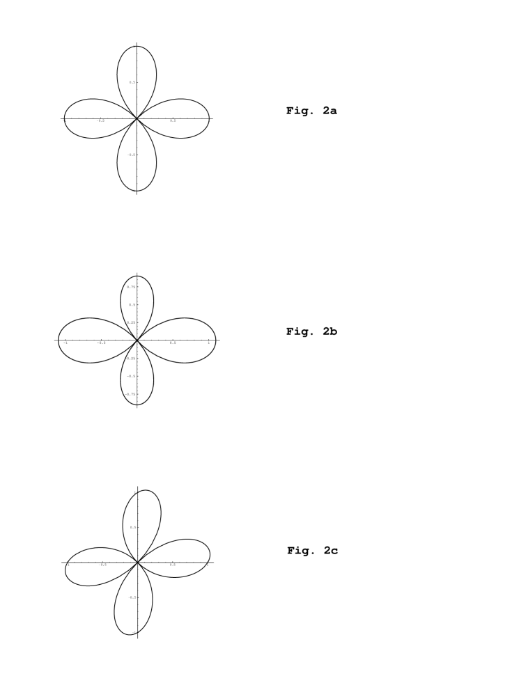
FIG. 2.: (a) The $k$-space structure of the superconducting order parameter with: (a) pure $d_{x^{2}-y^{2}}$ symmetry [$\cos(2\phi)$] ; (b) mixed $d_{x^{2}-y^{2}}$ and $s$ symmetry [$\cos(2\phi)+0.1$] ; (c) mixed $d_{x^{2}-y^{2}}$ and $d_{xy(x^{2}-y^{2})}$ symmetry [$\cos(2\phi)+0.3\sin(2\phi)\cos(2\phi)$]. Note that for the purpose of illustration, the magnitude of the $s$-wave component in Fig. (b) has been chosen to be larger than that expected from microscopic estimates (see the main text).

- [1] Electronic address: zapotock@uiuc.edu Address after September 1, 1996: Department of Physics and Astronomy, University of Pennsylvania, 209 South 33rd Street, Philadelphia, PA 19104-6396.
- [2] Electronic address: maslov@uiuc.edu Address after September 1, 1996: Department of Physics, University of Florida, 215 Williamson Hall, Gainesville, FL 32611-0524.
- [3] Electronic address: goldbart@uiuc.edu
- [4] D. A. Wollman, D. J. Van Harlingen, W. C. Lee, D. M. Ginsberg, and A. J. Leggett, Phys. Rev. Lett. 71, 2143 (1993); D. J. Van Harlingen, Rev. Mod. Phys. 67, 515 (1995).
- [5] W. N. Hardy, D. A. Bonn, D. C. Morgan, R. Liang, and K. Zhang, Phys. Rev. Lett. 70, 3999 (1993).
- [6] K. A. Moler, D. J. Baer, J. S. Urbach, R. Liang, W. N. Hardy, and A. Kapitulnik, Phys. Rev. Lett. 73, 2744 (1994).
- [7] J. Annett, N. Goldenfeld, and A. J. Leggett, to appear in Physical Properties of High Temperature Superconductors, Vol. 5, D. M. Ginsberg (ed.), (World Scientific, Singapore, 1996), and Report No. cond-mat/9601060.
- [8] R. Joynt, Phys. Rev. B 41, 4271 (1990).
- [9] Note that although the terms and transform separately as scalars, they are related through integration by parts.
- [10] J. F. Annett, Adv. Phys. 39, 83 (1990).
- [11] G. E. Volovik, Pis’ma Zh. Eksp. Teor. Fiz. 58, 457 (1993) [JETP Lett. 58, 469 (1993)].
- [12] P. I. Soininen, C. Kallin, and A. J. Berlinsky, Phys. Rev. B 50, 13883 (1994).
- [13] Y. Ren, J. H. Xu, and C. S. Ting, Phys. Rev. Lett. 74, 3680 (1995).
- [14] M. Franz, C. Kallin, P. I. Soininen, A. J. Berlinsky, and A. L. Fetter, Report No. cond-mat/9509154.
- [15] This assumption is valid, e.g., for the case of a wire of thickness less than the penetration depth , with current passed along the wire. It is also satisfied in a film (grown in the direction) of thickness and width [T. R. Lemberger, in Physical Properties of High Temperature Superconductors, Vol. 3, D. M. Ginsberg (ed.), (World Scientific, Singapore, 1996), and references therein]. In a film of width larger than , the distribution of the current and the magnetic field becomes strongly peaked at the edges of the film, leading to the nucleation of vortices and antivortices. Such a situation is not adequately described by the theory presented by us here.
- [16] L. J. Buchholtz, M. Palumbo, D. Rainer, and J. A. Sauls, Report No. cond-mat/9511027.
- [17] P. G. de Gennes, Superconductivity of Metals and Alloys (W. A. Benjamin, New York, 1966).
- [18] The four unknown quantities , , and satisfy four independent equations: of these, two are the Ginzburg-Landau equations, (2,3), and the remaining two arise from the condition that the perturbations do not alter the external current in Eq. (5). To arrive at Eq. (13), we first eliminate the quantity from Eqs. (5) and (2) to obtain the intermediate result: . Then, we eliminate the quantity from Eqs. (5) and (3), thus obtaining Eq. (13).
- [19] The corresponding Ginzburg-Landau parameters were also recently derived from two microscopic lattice models (the extended Hubbard model and the antiferromagnetic van Hove model) in the work of D. L. Feder and C. Kallin (unpublished). The use of their results instead of the results of Ren et al. does not significantly alter our quantitative estimates.
- [20] P. Monthoux and D. Pines, Phys. Rev. B 47, 6069 (1993).
- [21] L. D. Landau and E. M. Lifshitz, Quantum Mechanics: Non-Relativistic Theory (Pergamon Press, Oxford, 1977).