Transport in a one-dimensional Luttinger liquid

Abstract

In this paper we review recent theoretical results for transport in a one-dimensional (1d) Luttinger liquid. For simplicity, we ignore electron spin, and focus exclusively on the case of a single-mode. Moreover, we consider only the effects of a single (or perhaps several) spatially localized impurities. Even with these restrictions, the predicted behavior is very rich, and strikingly different than for a 1d non-interacting electron gas. The method of bosonization is reviewed, with an emphasis on physical motivation, rather than mathematical rigor. Transport through a single impurity is reviewed from several different perspectives, as a pinned strongly interacting “Wigner” crystal and in the limit of weak interactions. The existence of fractionally charged quasiparticles is also revealed. Inter-edge tunnelling in the quantum Hall effect, and charge fluctuations in a quantum dot under the conditions of Coulomb blockade are considered as examples of the developed techniques.

I Introduction

Landau’s Fermi liquid theory is a beautiful and successful theory which accounts for the behavior of the conduction electrons in conventional metallic systems[1]. The central assumption of this theory, is that the low energy excited states of the interacting electron gas can be classified in the same way as a reference non-interacting electron gas. Upon adiabatically “switching on” the electron interactions, the excited states are still composed of free quasiparticles, labelled by momentum, which obey Fermi statistics. The low energy excitations above the ground state, consist of creating quasiparticles (and quasiholes) with momenta just above (below) the Fermi surface. The single-particle spectral function for an electron is presumed to have a $\delta$-function peak at the Fermi surface, ${{\cal A}}(k_{F},\epsilon)=2\pi Z_{F}\delta(\epsilon)$, with a non-zero coefficient, $Z_{F}$. For the non-interacting electron gas $Z_{F}=1$, but with interactions $Z_{F}<1$, reflecting a smaller overlap between the electron and the quasiparticle. However, provided $Z_{F}$ is non-zero, there exist well defined low energy quasiparticle excitations, which are in a one-to-one correspondence with the bare electron excitations of the reference non-interacting electron gas. It is then possible to build a transport theory of Fermi liquids in direct analogy with Drude theory of the free electron gas, by focussing on the scattering (by impurities, say) of the low energy quasiparticle excitations. For example, a quasiparticle will scatter off an impurity with a finite cross-section, leading to a metallic resisitivity for low impurity concentration.

For a weakly-interacting electron gas, deviations in the spectral weight $Z_{F}$ from one can be computed perturbatively in the interaction strength, provided the spatial dimensionality, $d$, is greater than one. However, for the one-dimensional interacting system, low order terms in the perturbation theory are divergent. This signals the breakdown of Landau’s Fermi liquid theory in the 1d electron gas, for arbitrarily weak interactions[2]. This divergence can be traced to the large phase space in 1d, for an electron to relax by creating an electron-hole excitation. For $d>1$, both energy and momentum conservation highly constrain the available phase space, but in 1d for a single branch with linear dispersion, momentum conservation automatically implies energy conservation, so the phase space is less constrained. This leads to a divergent rate for such scattering processes, and the electron becomes “dressed” by a large number of electron-hole pairs. This in turn drives the electron spectral weight to zero, $Z_{F}=0$, even for weak electron interactions. In the limit of weak interaction, it is still possible to extract the resulting properties of the 1d electron gas by a clever resummation of the most divergent terms in each order of perturbation theory[3]. However, the physics is more readily revealed by the method of bosonization, as discussed below.

Tomonaga[4] (and more recently Luttinger[5]) considered a special class of interacting 1d electron models, which were linearized around the Fermi points, and could be diagonalized in terms of boson variables. These boson variables described collective plasmon excitations, or density waves, in the electron gas. Some years later, Haldane[6] argued that this bosonized decription was valid more generally, giving an appropriate description for the low energy excitations of a generic 1d interacting electron gas. Haldane coined the term “Luttinger liquid” to describe this generic behavior, although sometimes it is referred to as a Tomonaga-Luttinger liquid. In such a 1d Luttinger liquid, creation of a real electron is achieved by exciting an infinite number of plasmons. Because of this, the space and time dependence of the electron correlation function is dramatically different than in a non-interacting electron gas, or in a Fermi liquid[7]. This manifests itself in various kinetic quantities, in particular the Drude conductivity, which is predicted to vary (as a power law) with temperature[8, 9, 10]. The Luttinger liquid approach to transport in 1d systems was popular in the 1970‘s, being employed in attempts to understand the behavior of quasi-1d organic conductors.

Recent advances in semiconductor technology have renewed interest in transport of 1d electron systems. By cleverly “gating” a high mobility two-dimensional (2d) electron gas, it is possible to further confine the motion of the electrons, so that they can only move freely along a 1d channel. Moreover, it is possible to make a very narrow channel, with width comparable to the electron‘s Fermi wavelength. In this case, the transverse degrees of freedom are quantized, and only one, or perhaps several, 1d channels are occupied at the Fermi level. This “quantum wire” provides an experimental realization of a 1d electron gas, which should reveal the signatures of Luttinger liquid behavior without the complicated crossovers to three-dimensional behavior inherent in the quasi-1d organic conductors.

Edge states formed at the boundaries of the 2d electron gas when placed in strong magnetic field in the quantum Hall regime, provide another important example of a one-dimensional electron system[11]. These edge excitations are chiral, moving only in one direction along the edge. For a quantum Hall bar geometry, the two edge modes confined to the edges move in opposite directions. Together they comprise a non-chiral system, which resembles a 1d electron gas. For the integer quantum Hall effect, these edge excitations are equivalent to a 1d non-interacting electron gas, (despite the presence of electron interactions). However, in the fractional quantum Hall effect, the edge excitations are believed to be isomorphic to a 1d interacting Luttinger liquid[12]. Moreover, due to the spatial separation between the modes on opposite edges, impurities cannot backscatter, so that localization effects important in a quantum wire are absent here.

A 1d quantum wire is appropriately characterized by a conductance, which can be measured in a transport experiment. In the absence of interactions, the conductance of an ideal single-mode channel wire, adiabatically connected[13] to leads, is quantized, $G=2e^{2}/h$ – where the factor of 2 accounts for spin. If a scatterer is introduced into the channel, the conductance drops, with $G=2{\cal T}e^{2}/h$– where ${{\cal T}}<1$ is the transmission coefficient for electrons at the Fermi level. For edge states in the integer quantum Hall effect, a quantized conductance occurs when there is no backscattering between modes on opposite edges, and corresponds to the quantized Hall conductance. Inter-edge scattering is equivalent to a reduced transmission coefficient, and reduces the conductance.

As discussed above, electron interactions should dramatically modify the low energy excitations in the quantum wire. As we shall see, this leads to striking predictions for the transport in a quantum wire with one or several impurities. Likewise, inter-edge backscattering in the fractional quantum Hall effect is predicted to be very different than in the integer Hall effect.

In this paper we review recent theoretical results for transport in a 1d Luttinger liquid. For simplicity, we ignore electron spin, and focus exclusively on the case of a single-mode. Moreover, we consider only the effects of a single (or perhaps several) spatially localized impurities. As we shall see, even with these restrictions, the predicted behavior is very rich, and strikingly different than for a 1d non-interacting electron gas.

The paper is organized as follows. In Section II the method of bosonization is reviewed, with an emphasis on physical motivation, rather than mathematical rigor. After discussing briefly the conductance of an ideal channel, we reveal the existence of fractionally charged excitations in the Luttinger liquid. These correspond to Laughlin quasiparticles for fractional quantum Hall edge states, but should also be present in quantum wires. In Section III, we consider the tunnelling density of states for adding an electron into a 1d Luttinger liquid, which is suppressed, vanishing as a power law of energy. The exponent is extracted for both tunnelling into the middle of an infinite 1d wire, and into the “end” of a semi-infinite wire. Section IV is devoted to a detailed analysis of transport in a Luttinger liquid with a single barrier or impurity. We consider two limiting cases, a very large barrier in IVA and a very small barrier in IVB. In Section IVC we show how the crossover between these two limits can be understood by considering general barrier strengths, but weak electron interactions. A general picture of this crossover is described in IVD, and the special case of resonant tunnelling is discussed in IVE.

In Section V, we consider briefly two particular applications. In VA we consider tunnelling between edge states in the fractional quantum Hall effect, which is a rather straightforward application of the general theory. In Section VB we employ Luttinger liquid theory to describe Coulomb blockade in a quantum dot. Section VI is devoted to a very brief summary, and list of other related topics.

II Bosonization

Consider the Hamiltonian for spinless electrons hopping on a 1d lattice,

$${\cal H}=-t\sum_{j}c_{j}^{\dagger}c_{j+1}+h.c.+{\frac{V}{2}}\sum_{j}c_{j}^{\dagger}c_{j}c_{j+1}^{\dagger}c_{j+1},$$ (1)

with hopping strength $t$ and near-neighbor interaction strength $V$. When $V=0$ one can diagonalize the problem in terms of plane waves with energy $E_{k}=-t\cos(k)$ for momentum $k$ satisfying $|k|<\pi$. The low energy excitations consist of particle/hole excitations across the two Fermi points, at $\pm k_{F}$. Consider a single particle hole/excitation about the right Fermi point, where a single electron is removed from a state with $k<k_{F}$ and placed into an unoccupied state with $k+q>k_{F}$. For small momentum change $q$, the energy of this excitation is $\omega_{k}=v_{F}q$, with $v_{F}$ the Fermi velocity. Together with the negative momentum excitations about the left Fermi point, this linear dispersion relation is identical to that for phonons in one-dimension. The method of Bosonization exploits this similarity by introducing a phonon displacement field, $\theta$ to decribe this linearly dispersing density wave. When interactions are turned on, the single particle nature of the excitations is not retained, but this linearly dispersing mode survives, with a renormalized velocity.

The method of Bosonization focusses on the low energy excitations, and provides an effective theory. We follow the heuristic development of Haldane[6], which reveals the important physics, dispensing with mathematical rigor. To this end, consider a Jordan-Wigner transformation which replaces the electron operator, $c_{j}$, by a (hard-core) boson operator, $c_{j}=\exp(i\pi\sum_{j<i}n_{i})b_{j}$, where $n_{j}=c^{\dagger}_{j}c_{j}$ is the number operator. One can easily verify that the Bose operators commute at different sites. Moreover, the above Hamiltonian when re-written is of the identical form with $c^{\prime}s$ replaced by $b^{\prime}s$. This transformation, exchanging Fermions for Bosons, is a special feature of one-dimension. The Boson operators can be (approximately) decomposed in terms of an amplitude and a phase, $b\rightarrow\sqrt{n_{j}}\exp(i\phi_{j})$. We now imagine passing to the continuum limit, focussing on scales long compared to the lattice spacing. In this limit we replace, $\phi_{j}\rightarrow\phi(x)$ and $n_{j}\rightarrow\rho(x)$, where $\rho(x)$ is the 1d electron density. This can be decomposed as $\rho=\rho_{0}+\tilde{\rho}$, where the mean density, $\rho_{0}=k_{F}/\pi$, and $\tilde{\rho}$ is an operator measuring fluctuations in the density. As usual, the density and phase are canonically conjugate quantum variables, taken to satisfy

$$[\phi(x),\tilde{\rho}(x^{\prime})]=i\delta(x-x^{\prime}).$$ (2)

Now we introduce a phonon-like displacement field, $\theta(x)$, via $\tilde{\rho}(x)=\partial_{x}\theta(x)/\pi$. The factor of $\pi$ has been chosen so that the full density takes the simple form: $\rho(x)=(k_{F}+\partial_{x}\theta)/\pi$. The above commutation relations are satisfied if one takes,

$$[\phi(x),\theta(x^{\prime})]={{i\pi}\over{2}}{\rm sgn}(x-x^{\prime}).$$ (3)

Notice that $\partial_{x}\phi$ is the momentum conjugate to $\theta$. The effective (Bosonized) Hamiltonian density which describes the 1d density wave takes the form:

$$H={v\over{2\pi}}[g(\partial_{x}\phi)^{2}+g^{-1}(\partial_{x}\theta)^{2}].$$ (4)

This Hamiltonian describes a wave propagating at velocity $v$, as can be readily verified upon using the commutation relations to obtain the equations of motion, $\partial_{t}^{2}\theta=v^{2}\partial_{x}^{2}\theta$, and similarly for $\phi$. For non-interacting electrons one should equate $v$ with the (bare) Fermi velocity, $v_{F}$, but with interactions $v$ will be modified (see below). The additional dimensionless parameter, $g$, in the above Hamiltonian also depends on the interaction strength. For non-interacting electrons one can argue that $g=1$, as follows. A small variation in density, $\tilde{\rho}$ will lead to a change in energy, $E=\tilde{\rho}^{2}/2\kappa$, where $\kappa=\partial\rho/\partial\mu$ is the compressibility. Since $\partial_{x}\theta=\pi\tilde{\rho}$, one deduces from $H$ that $\kappa=g/\pi v$. But for a non-interacting electron gas, $\pi v\kappa=1$, so that $g=1$.

To see why $g$ shifts with interactions, it is convenient first to identify the electron creation operator. On physical grounds, the appropriate operator, denoted $\psi^{\dagger}(x)$, should create a unit charge ($e$) excitation at point $x$, which anti-commutes with the same operator at a different point $x^{\prime}$. Consider the Bose creation operator, $b^{\dagger}\sim\exp(i\phi)$. To see that this indeed creates a unit charge ($e$) excitation, one can write,

$$e^{i\phi(x)}=e^{i\pi\int_{-\infty}^{x}dx^{\prime}P(x^{\prime})},$$ (5)

where $P=\partial_{x}\phi/\pi$ is the momentum conjugate to $\theta$. Since the momentum operator is the generator of translations (in $\theta$), this creates a kink in $\theta$ of height $\pi$ centered at position $x$. This corresponds to a localized unit of charge, since the density $\tilde{\rho}=\partial_{x}\theta/\pi$.

To construct an electron operator requires multiplying the Bose operator $e^{i\phi}$ by a Jordan-Wigner “string”: $e^{i\pi\sum_{j<i}n_{i}}\rightarrow e^{i\pi\int^{x}\rho}$. Rewriting in terms of $\theta$, this corresponds to $e^{i(k_{F}x+\theta)}$. The most general Fermionic charge $e$ operator can thus be written,

$$\psi(x)=\sum_{m_{\rm odd}}\psi_{m}\approx\sum_{m_{\rm odd}}e^{im(k_{F}x+\theta(x))}e^{i\phi(x)}.$$ (6)

The requirement that the integer $m$ is odd is dictated by Fermi statistics, since one can show using the commutation relations, that

$$\psi_{m}(x)\psi_{m^{\prime}}(x^{\prime})=e^{i\pi(m-m^{\prime}){\rm sgn}(x-x^{\prime})}\psi_{m^{\prime}}(x^{\prime})\psi_{m}(x).$$ (7)

The terms with $m=\pm 1$ have a very simple interpretation. The electron field operator has been expanded into a right and left moving piece, corresponding to the right and left Fermi points at $\pm k_{F}$:

$$\psi(x)\approx\psi_{R}+\psi_{L}\approx e^{ik_{F}x}e^{i\Phi_{R}}+e^{-ik_{F}x}e^{i\Phi_{L}},$$ (8)

with the definition, $\Phi_{R/L}=\phi\pm\theta$. Here $\Phi_{R/L}$ describe the slowly varing piece of the electron field. These two fields commute with one another, and satisfy:

$$[\Phi_{R}(x),\Phi_{R}(x^{\prime})]=-[\Phi_{L}(x),\Phi_{L}(x^{\prime})]=i\pi{\rm sgn}(x-x^{\prime}).$$ (9)

Notice that these unusual commutation relations - referred to as Kac-Moody - imply that the field conjugate to $\Phi$ is the derivative of $\Phi$ itself. These fields are simply related to the right and left moving electron densities, denoted $N_{R/L}$, via

$$N_{R/L}=\pm{1\over{2\pi}}\partial_{x}\Phi_{R/L}.$$ (10)

Note that these densities sum to give the total density, $N_{R}+N_{L}=\tilde{\rho}$.

It is instructive to re-write the Hamiltonian (4) in terms of the right and left electron densities,

$$H=\pi v_{0}[N_{R}^{2}+N_{L}^{2}+2\lambda N_{R}N_{L}],$$ (11)

with

$$v_{0}=v(g+g^{-1})/2$$ (12)

$$\lambda=(1-g^{2})/(1+g^{2}).$$ (13)

This Hamiltonian descibes the system of right- and left-moving electrons with the interaction strength $\lambda$ between the two species. Notice that for $g=1$ the interaction vanishes, and $v_{0}=v$; Hamiltonian (11) then gives the Bosonized decsription of the non-interacting electron gas, and $v_{0}\equiv v_{F}$, the bare Fermi velocity. Repulsive interactions, ($\lambda>0$) correspond to $g<1$, whereas attractive interactions give $g>1$.

Since Hamiltonians (4) and (11) give only an effective low energy description, it is generally difficult to relate the velocity $v$, and the interaction parameter $g$, to the bare interaction strength in the original lattice model, say Eqn. (4). However, for a model with long-range electron-electron interactions (Tomonaga model, see e.g., Ref. [[7]]) these relations can be obtained analytically. In the Tomonaga model, only Fourier components with $k\ll k_{F}$ of the interaction potential $V(k)$ are taken into account, and the parameters in Eqs. (4) and (11) can be expressed[7] in terms of $V(0)$. We consider here a generalized Tomonaga model, which allows for different values of interaction between the electrons moving in the same direction ($V_{ll}(0)=V_{rr}(0)\equiv V_{1}$) and in opposite directions ($V_{lr}(0)=V_{rl}(0)\equiv V_{2}$). The velocity $v$ and interaction parameter $g$ can be related to $V_{1}$ and $V_{2}$ as follows. In the generalized Tomonaga model, the energy associated with a density fluctuation in the right- or left-moving mode ($N_{R}$ or $N_{L}$) is a sum of two terms, representing compressibility of the non-interacting Fermi gas, and the interaction potential $V_{1}$, respectively. Equating this with the coefficient of $N_{R}^{2}$ in 11, gives: $\pi v_{0}=\pi v_{F}+V_{1}$. The interaction between the modes $V_{2}$ is responsible for the last term in Eq. (11), so that $\pi v_{0}\lambda=V_{2}$. These two relations can be used to solve for the velocity $v$ and parameter $g$, giving[15]

$$v=v_{F}\left(1+\frac{V_{1}}{\pi v_{F}}+\frac{V_{1}^{2}-V_{2}^{2}}{4\pi^{2}v_{F}^{2}}\right)^{1/2},$$ (14)

$$g=\left(\frac{1+V_{1}/2\pi v_{F}-V_{2}/2\pi v_{F}}{1+V_{1}/2\pi v_{F}+V_{2}/2\pi v_{F}}\right)^{1/2}.$$ (15)

In the conventional case $V_{1}=V_{2}>0$, and $v$ is simply the plasmon velocity, increasing above $v_{F}$ with repulsive interactions which reduce the compressibility of the electron gas. Notice, moreover, that the sign of $1-g$ is determined by the sign of the interaction, with $g<1$ for repulsive interactions. Edge states propogating on opposite edges of an integer quantum Hall bar, constitute a 1d system with $V_{1}>V_{2}$. In particular, for a wide Hall bar, the inter-edge interaction $V_{2}$ vanishes, so that $g=1$ .

A Meaning of g

No matter what the underlying microscopic model is, the parameter $g$ of the Luttinger liquid (4) can be given a simple physical meaning as a dimensionless conductance. To this end we define new variables $\phi_{R/L}=g\phi\pm\theta$ which decouple the right and left moving sectors, and at the same time diagonalize the Hamiltonian (4). The corresponding right and left moving densities are

$$n_{R/L}=\pm{1\over{2\pi}}\partial_{x}\phi_{R/L}.$$ (16)

Although $n_{R/L}$ again sum to give the total density, $n_{R}+n_{L}=\tilde{\rho}$, for $g\neq 1$ they do not correspond to the right and left pieces of an electron, but rather involve contributions from electrons propagating in both directions. The right and left fields commute with one another and satisfy,

$$[\phi_{R}(x),\phi_{R}(x^{\prime})]=-[\phi_{L}(x),\phi_{L}(x^{\prime})]=i\pi g{\rm sgn}(x-x^{\prime}),$$ (17)

the same as for $N_{R/L}$ except with an important factor of $g$ on the right side. In terms of these fields, the Bosonized Hamiltonian decouples into right and left moving sectors:

$$H={{\pi v}\over g}[n_{R}^{2}+n_{L}^{2}].$$ (18)

This innocent looking decoupling, leads to a number of remarkable predictions for the 1d electron gas, as discussed below. Firstly, from the Hamiltonian one can generate the equations of motion, which are

$$(\partial_{t}\pm v\partial_{x})n_{R/L}=0.$$ (19)

These chiral wave equations have the general solutions, $n_{R/L}=f(x\mp vt)$, for arbitrary $f$, and describe a density disturbance which propagates, without scattering (or dispersion), to the right or left. This, despite the fact that the electrons, which are interacting, do scatter off one another.

The physical meaning of $g$ as a conductance can now be revealed. Imagine an external probe (or contact) which raises the chemical potential of the chiral mode $n_{R}$, by an amount $\mu_{R}$. This can be incorporated by adding to the Hamiltonian density a term of the form, $\delta H=-e\mu_{R}n_{R}$. This leads to a shift in the right moving density, since the total Hamiltonian is no longer minimized by $n_{R}=0$. Rather, minimization with respect to $n_{R}$, gives $n_{R}=(ge/2\pi v)\mu_{R}$. This extra density carries an additional (transport) current to the right, of magnitude, $I_{R}=en_{R}v$. One thus has, $I_{R}=G\mu$ with a conductance,

$$G=g{{e^{2}}\over h}.$$ (20)

For non-interacting electrons ($g=1$), we recover the result of Landauer transport theory – $e^{2}/h$ conductance per channel. But with interactions $G$ is modified.

Unfortunately, in a quantum wire, it is essentially impossible to selectively couple to the right moving mode $n_{R}$, and not the left. Rather, in a typical transport experiment, the quantum wire is connected at its ends to bulk metallic contacts, which can be modelled as free electron gases (Fermi-liquids). In this case, the dc transport will be sensitive to the contacts. This can be seen by considering an alternative derivation of Eq. (20), based on linear response theory. Consider an ac electric field $E(x,t)=-U^{\prime}(x)\sin\omega t$, applied along an infinite wire, which is non-zero for $x$ near the origin, say $|x|<L/2$. This leads to a term of the form $geE(x,t)$ on the right hand side of (19). This field will cause an excitation of density waves $n_{R/L}(x,t)$, which propogate along the wire. For $\omega<v/L$, the wavelength of the excitation becomes much larger than $L$, so that one may then substitute $U^{\prime}(x)=-U\delta(x)$, with $U$ the amplitude of the applied ac voltage across the length $L$ segment. The equations of motion can now be readily solved, giving for the current response, $I(x,t)=ge^{2}U\cos\omega[t-xsgn(x)/v]$. Although the current depends on $x$, this dependence vanishes in the $\omega\to 0$ limit, and gives a dc conductance $G=I/U=ge^{2}/h$, which reproduces Eq. (20). The conductance is clearly related to the energy radiated away from the length $L$ segment. Indeed, the radiated energy per unit time is exactly equal to the power $U^{2}G/2$ absorbed from the field. The resulting conductance is finite, even in the absence of any disorder. It is clear from this arguemnt that the dc conductance, proportional to the power radiated away, depends on the value of $g$ in the segment of wire away from the length $L$ region. For a wire of length $L$ attached (adiabatically) to Fermi liquid leads, one can take $g=1$ in the leads[16], and one then expects a dc conductance given by $G=e^{2}/h$. The value of $g\neq 1$ in the wire, can be revealed by an a.c. conductance measurement for frequencies $\omega>v/L$, which has magnitude[17][18] $G(\omega)=ge^{2}/h$.

There is a physical system however, in which the right and left modes, $n_{R/L}$ can be coupled to selectively. As discussed in more detail in Section V A below, in the fractional quantum Hall effect (FQHE) at such filling factors $\nu<1$, that $\nu^{-1}$ is an odd integer, a single current carrying mode is predicted along the sample edges. In a Hall bar geometry, the right and left moving modes are localized on the top and bottom edges of the sample, respectively. These modes are mathematically isormorphic to the right and left moving modes of the 1d interacting electron gas, $n_{R/L}$, provided one makes the identification $g=\nu$. In the FQHE geometry, a chemical potential difference between the right and left moving modes, corresponds to a Hall potential drop, transverse to the transport current. The above conductance, corresponds directly to the quantized Hall conductance, $G=\nu e^{2}/h$.

B Charge fractionalization

The above analogy with the FQHE, suggests the possibility of fractionally charged excitations in the 1d electron gas. To see these, it is convenient to consider adding a small impurity potential, localized at the origin $x=0$. This potential will cause scattering between the right and left moving modes, $n_{R/L}$. We shall now show that the “particle” which is backscattered is not a (bare) electron. Rather, the total backscattered charge is non-integral, with magnitude $ge$. For repulsive interactions $g<1$, this corresponds to the backscatering of a quasiparticle with fractional electron charge. We shall also show, that this fractionally charged quasiparticle, also has fractional statistics. A localized impurity potential, $U(x)=u\delta(x)$, couples to the local electron density, $\psi^{\dagger}(0)\psi(0)$. Inserting the expression (8), gives the dominant $2k_{F}$ backscattering contribution:

$$H_{\rm imp}=u\delta(x)(\psi^{\dagger}_{R}\psi_{L}+h.c.)=u\delta(x)(e^{i2\theta}+h.c.).$$ (21)

Although, this perturbation backscatters a (bare) electron, there is a “backflow” term due to the electron-interactions. To reveal this, one should re-express the above perturbation in terms of the fields, $\phi_{R/L}$, which propogate freely (to the right or left) even in the presence of electron interactions. One gets simply,

$$H_{\rm imp}=u\delta(x)(e^{i\phi_{R}}e^{-i\phi_{L}}+h.c.),$$ (22)

so that the impurity hops an $e^{i\phi_{R/L}}$ quasiparticle between the two modes. The charge created by the operator $e^{i\phi_{R}}$ can be deduced from the conjugate momentum, $P_{R}=\partial_{x}\phi_{R}/2\pi g$ which follows from the commutation relations (17). One has,

$$e^{i\phi_{R}(x)}=e^{i2\pi g\int^{x}P_{R}(x^{\prime})},$$ (23)

which creates a kink in $\phi_{R}$ of magnitude $2\pi g$ centered at $x$. Since $n_{R}=\partial_{x}\phi_{R}/2\pi$ the charge associated with this (kink) excitation is fractional, $Q=ge$.

Thus, a localized impurity potential in an interacting 1d electron gas, causes backscattering of fractionally charged quasiparticles ($Q=ge$) between the free-streaming right and left moving modes, $n_{R/L}$. In the FQHE, a localized impurity is equivalent to a “point contact” in which the right and left moving edge modes on opposite sides of the Hall bar are “pinched” together, to allow for inter-mode backscattering. In this case, these backscattered quasiparticles have a natural physical interpretation as Laughlin quasiparticles with charge $Q=\nu e$. The fractional charge can perhaps be revealed in a shot noise type experiment, as discussed in Ref. [19].

Not surprisingly, these quasiparticle excitations also have fractional statistics. To see this we can use the commutation relations (17) to show that,

$$e^{i\phi_{R}(x)}e^{i\phi_{R}(x^{\prime})}=e^{i\pi g{\rm sgn}(x-x^{\prime})}e^{i\phi_{R}(x^{\prime})}e^{i\phi_{R}(x)},$$ (24)

so that under exchange they pick up a phase factor $\exp(i\pi g)$. For the non-interacting electron gas, $g=1$, the quasiparticles have charge $e$ and Fermi statistics (the electron!), but with interactions will have fractional statistics.

III Tunnelling into a Luttinger liquid

As discussed in the previous section, elementary excitations in the Luttinger liquid are significantly different from bare electrons. This difference reveals itself in the behavior of the density of states for tunnelling an electron into the Luttinger liquid. In subsection A below we will consider specifically the local tunnelling density of states for an infinitely long Luttinger liquid. Another situation of interest, analyzed in subsection B, consists of tunnelling an electron through a large barrier separating two semi-infinite systems. This process is sensitive to the density of states at the “end” of a semi-infinite Luttinger liquid, which, in contrast to the non-interacting electron gas, behaves differently than the “bulk” density of states.

Since the effective Hamiltonian density (4) is quadratic in the boson fields, local density of states can be readily extracted. Perhaps the simplest way to proceed, is to represent the partition function,

$$Z={\rm Tr}\exp(-\beta\int_{x}H),$$ (25)

as an imaginary time path integral over the boson fields:

$$Z=\int D\phi D\theta\exp(-S),$$ (26)

where the integration is over classical fields $\phi(x,\tau)$, and similarly $\theta$, with imaginary time $\tau$ running from $0$ to $\beta$. The (Euclidian) action can be written in terms of the Lagrangian, $S=\int dxd\tau{\cal L}_{0}$, with

$${\cal L}_{0}={i\over\pi}\partial_{\tau}\phi\partial_{x}\theta+H(\phi,\theta),$$ (27)

with $H$ given in (4). It is instructive to perform the (Gaussian) functional integration over, say $\phi$, which gives:

$${\cal L}_{0}^{\theta}={1\over{2\pi g}}[v(\partial_{x}\theta)^{2}+v^{-1}(\partial_{\tau}\theta)^{2}],$$ (28)

describing, via the “displacement” field $\theta$, 1d phonons propagating with velocity $v$. Likewise, integration over $\theta$ gives:

$${\cal L}_{0}^{\phi}={g\over{2\pi}}[v(\partial_{x}\phi)^{2}+v^{-1}(\partial_{\tau}\phi)^{2}].$$ (29)

This can be interpreted as a wave propagating in the phase-field $\phi$. Notice that $g\rightarrow g^{-1}$ upon transforming between the two representations, $\theta\rightarrow\phi$. At the special non-interacting point, $g=1$, there is a self-duality between these two representations. Physically, for strong repulsive interactions corresponding to $g<<1$, (zero-point) fluctuations in the displacement field $\theta$ are greatly suppressed. In this limit $\theta$ becomes a “good” classical variable, and the 1d electron system is well described as a “solid” - or equvalently a Wigner crystal. In the opposite extreme of very strong attractive interactions, $g>>1$, fluctuations in the phase $\phi$ are strongly suppressed. The system is well described as a (almost) condensed superfluid of the (Jordan-Wigner) bosons, $b$.

In the presence of a single impurity, the Hamiltonian $H(\phi,\theta)$ in Eq. (27) should be replaced by $H+H_{\rm imp}$. Using Eq. (21) and integrating out the field $\phi$, we find

$${\cal L}^{\theta}={1\over{2\pi g}}[v(\partial_{x}\theta)^{2}+v^{-1}(\partial_{\tau}\theta)^{2}]+u\delta(x)(e^{2i\theta}+h.c.).$$ (30)

In the language of 1d displacements, the impurity plays the role of a pinning center, which favors a periodic set of values of the displacement field at the pinning site. A strong center (large $|u|$) effectively cuts the infinite system in two semi-infinite pieces with independent excitation spectra. Each piece is then described by the Lagrangian (28), defined on the appropriate semi-infinite space with boundary condition $\theta(x=0)=0$.

A Tunneling into a clean Luttinger liquid

Consider now the local electron tunnelling density of states for adding an electron at energy $E$,

$$\rho(E)=2\pi\sum_{n}|<n|\psi^{\dagger}(x)|0>|^{2}\delta(E_{n}-E_{0}-E).$$ (31)

Here $|n\rangle$ are exact eigenstates of the full interacting Hamiltonian, and $E_{n}$ are the corresponding energies. The summation in Eq. (31) is performed over a complete set of states, and therefore with the help of the identity

$$\delta(E_{n}-E_{0}-E)=\frac{1}{\pi}{\rm Re}\int_{0}^{\infty}dte^{i(E+E_{0}-E_{n})t},$$ (32)

can be related to the electron Green’s function,

$$\rho(E)=\frac{1}{\pi}{\rm Re}\int_{0}^{\infty}dte^{iEt}\langle\psi(x,t)\psi^{\dagger}(x,0)\rangle.$$ (33)

This can be evaluated by computing the imaginary time correlator,

$${\cal G}(\tau)=\langle T_{\tau}\psi(\tau)\psi^{\dagger}(0)\rangle,$$ (34)

and then performing an analytic continuation, $\langle\psi(t)\psi^{\dagger}(0)\rangle={\cal G}(\tau\rightarrow it)$.

Upon re-expressing the electron operator in terms of the boson fields, using (8), the average in (34) can be readily performed for a system with a quadratic Lagrangian. For a clean infinite 1d system, one can use the Lagrangian (27). With a frequency cutoff, $\tau_{c}^{-1}$, one finds,

$${\cal G}(\tau)=\left({\tau_{c}\over{|\tau|+\tau_{c}}}\right)^{\alpha},$$ (35)

with exponent $\alpha=(g+g^{-1})/2$. After analytic continuation and Fourier transformation, one thereby obtains,

$$\rho(E)={{2\pi}\over{\Gamma(\alpha)}}\Theta(E)\tau_{c}^{\alpha}E^{\alpha-1}.$$ (36)

Notice that for non-interacting electrons ($g=1$), one recovers the expected constant density of states. However, with interactions present, $g\neq 1$, the electron tunnelling density of states vanishes as $E\rightarrow 0$. This striking feature of the 1d electron gas is intimately related to the fractional charge. For $g\neq 1$ the excitations of the system are not free electron like, and there is an orthogonality catastrophe when one tries to add in an electron. The orthogonality catastrophe occurs because the accomodation of an added electron requires modification of the wavefunctions of all the electrons forming the liquid.

The tunneling conductance through a large barrier separating two semi-infinite Luttinger liquids, is proportional to the product of the “end” density of states for the two pieces. This can be evaluated with the help of the Lagrangian (29) defined, say, for $x>0$, together with the boundary condition $\theta(x=0)=0$. The result is similar to Eq. (36) with $\alpha=1/g$. This result can be understood in rather simpler physical terms in the limit of $g\ll 1$, as we now discuss.

B Tunneling through a barrier in the limit $g\ll 1$

In the limit of strong electron-electron interactions, the fluctuations in the “displacement” field are small, and the 1d system with a single barrier can be treated as a Wigner crystal pinned by an impurity. At low energies $E$, the process of tunneling consists of several stages.

If the barrier created by the impurity is narrow and high enough, tunneling of the electrons close to the barrier occur on a fast time scale, set by the Wigner crystal Debye frequency, $\omega_{D}\equiv k_{F}v$. This fast process results in a sudden ($|t|\lesssim 1/\omega_{D}$) creation of an electron vacancy–interstitial pair separated by the barrier. The energy of such a configuration is large, $\sim\omega_{D}/g$, and therefore the corresponding state of the Wigner crystal is classically forbidden. Gradual relaxation of the electron localized near the barrier, constitutes the slow stage of tunneling.

Complete relaxation requires that all the electrons of the Wigner crystal shift from their initial positions by one crystalline period. Since the overlap between the initial and final wave functions for each electron is suppressed, in the thermodynamic limit the initial and final many-body ground states are orthogonal to one other - the orthogonality catastrophe. This implies that the tunneling amplitude at $E=0$ vanishes. At $E>0$, a complete relaxation is not required, since the system can end up in an excited state. The initial ground state should have a non-vanishing overlap with the final excited state, and the tunneling amplitude is finite[20].

The density of states is directly related to the amplitude of the tunneling process for a semi-infinite Wigner crystal, after an interstitial is introduced at its edge, see Eq. (33). In the semiclassical approximation this amplitude can be expressed in terms of the action accumulated along the optimal classical trajectory,

$$\langle\psi(x,t)\psi^{\dagger}(x,0)\rangle\sim\exp[-S(t)].$$ (37)

As we now show, the slow stage of tunneling contributes a logarithmically divergent contribution[21] as $|t|\to\infty$. This divergence justifies the use of a (28) harmonic in deformations, and also enables one to treat the low-energy tunneling semiclassically, not only in the limit $g\ll 1$, but at any value of $g<1$.

Let us consider the evolution of the right half of the pinned Wigner crystal, $x>0$. To connect the initial local deformation $\tilde{\rho}(x,t=0)=2\delta(x)$ with the final relaxed state $\tilde{\rho}(x,t=\infty)=0$, the optimal trajectory must run in imaginary time, $t=i\tau$. The appropriate solution of the equations of motion gives

$$\tilde{\rho}(x,\tau)=\frac{2}{\pi}\frac{v\tau}{x^{2}+(v\tau)^{2}},\quad x>0.$$ (38)

This solution is applicable for sufficiently large $x^{2}+(v\tau)^{2}$, so that the harmonic description, see Eqs. (4), (28) is valid. Note that the dimensionless displacement at the origin, $\theta(x=+0,t)=-\pi$, remains constant in time, which allows us to use consistently the limit of a $\delta$-function in the initial condition. Eq. (38) describes the spread and relaxation of the deformation created by the tunnelling electron. The associated potential energy, $V_{\rm def}(\tau)$, decreases monotonically with time. Specifically, with the help of (38), one has:

$$V_{\rm def}(\tau)=\frac{v}{2\pi g}\int_{0}^{\tau}dx(\partial_{x}\theta)^{2}=\frac{2v}{\pi g}\int_{0}^{\tau}dx\frac{(v\tau)^{2}}{\left[x^{2}+(v\tau)^{2}\right]^{2}},$$ (39)

which gives $V_{\rm def}(\tau)=1/(2g\tau)$. The kinetic energy is equal to the potential energy (virial theorem), and thus we find

$$S(\tau)=2\int_{\omega_{D}^{-1}}^{\tau}V_{\rm def}(\tau)=\frac{1}{g}\ln(\omega_{D}\tau)$$ (40)

for the tunneling action. Here we have used $1/\omega_{D}$ as the short-time cut-off for the slow part of the evolution. Finally, upon using Eqs. (33) we can extract the tunnelling density of states, $\rho(E)\propto E^{\alpha-1}$ with $\alpha=1/g$.

IV Electron transport in a Luttinger liquid with a barrier

In the preceding Section we obtained the tunnelling density of states for adding an electron at energy $E$ into a Luttinger liquid. We considered two cases: Tunnelling into an infinite Luttinger liquid and tunnelling into the end of a semi-infinite system. In both cases the DOS vanished as a power law of energy for an electron gas with repulsive interactions. Here we consider an infinitely long interacting electron gas with a single defect or barrier, localized at the origin. Of interest is electron transport through the barrier. We first consider two limiting cases, a very large barrier in Subsection A, and a very small barrier in Subsection B. In Subsection C we show how the crossover between these two limits can be understood by considering general barrier strengths, but weak electron interactions. A general picture of the crossover is discussed in Subsection D. Finally, we consider the special case of resonant tunneling in Subsection E.

A Large Barrier

An infinitely high barrier breaks an electron gas into two de-coupled semi-infinite pieces. Each piece can be described by either of the quadratic Lagrangians, (28) or (29). For a very high, but finite barrier, we can consider electron tunnelling from one semi-infinite piece into the other as a perturbation. The appropriate tunnelling term to add to the Hamiltonian, is of the form

$$H_{\rm tun}=t_{0}[\psi_{1}^{\dagger}(x=0)\psi_{2}(x=0)+h.c.],$$ (41)

where $\psi_{1}$ ($\psi_{2}$) is the electron operator in the left (right) semi-infinite Luttinger liquid. Here $t_{0}$ denotes the (bare) tunnelling amplitude. Using (6) these operators can be readily expressed in terms of the boson fields, $\theta$ and $\phi$. However, with an infinitely high barrier the displacement field $\theta(x)$ is pinned at the origin, so one can take $\psi(x=0)=\exp[i\phi(x=0)]$.

The two-terminal conductance through the point contact can now be computed perturbatively for small tunneling amplitude $t_{0}$. In the presence of a voltage $V$ across the junction, the tunneling rate to leading order can be obtained from Fermi’s Golden rule:

$$I={2\pi e\over\hbar}\sum_{n}s_{n}|\langle n|H_{\rm tun}|0\rangle|^{2}\delta(E_{n}-E_{0}-s_{n}eV).$$ (42)

The sum on $n$ is over many-body states in which an electron has been transferred across the junction in the $s_{n}=\pm 1$ direction. It is straightforward to re-express this as

$$I={et^{2}_{0}\over 2\pi\hbar}\int dE\left[\rho_{1}^{>}(E)\rho_{2}^{<}(E-eV)-\rho_{1}^{<}(E-eV)\rho_{2}^{>}(E)\right]$$ (43)

where $\rho_{a}^{>}$ ($\rho_{a}^{<}$) is the tunneling densities of states for adding (removing) an electron at energy $E$. These are related by $\rho^{<}(E)=\rho^{>}(-E)$.

Upon using the expression (36) for the tunnelling DOS into the end of a semi-infinite Luttinger liquid, one readily obtains,

$$I\propto t^{2}_{0}|V|^{(2/g)-2}V,\quad G(V)\equiv\frac{dI}{dV}\propto t^{2}_{0}|V|^{(2/g)-2}.$$ (44)

For repulsive interactions ($g<1)$, the linear conductance is strictly zero! This is a simple reflection of the suppressed density of states in a Luttinger liquid. When $g=1$ a linear $I-V$ curve is predicted, consistent with expectations for non-interacting electrons which are partially transmitted through a barrier. At finite temperatures the density of states is sampled at $E\approx kT$, and a non-zero (linear) conductance is expected. Generalizing Fermi’s Golden rule to $T\neq 0$ gives the expected result for the (linear response) conductance:

$$G(T)\propto t^{2}_{0}T^{(2/g)-2}.$$ (45)

It is instructive to re-cast this result in the language of the renormalization group (RG). Specifically, the vanishing conductance for $g<1$ indicates that the tunneling perturbation, $t_{0}$, is irrelevant. The RG can be implemented using the Bosonized representation, in which the tunnelling term takes the form,

$$S_{\rm tun}=t_{0}\int d\tau e^{i\phi(\tau)},$$ (46)

with $\phi(\tau)=\phi_{1}(x=0,\tau)-\phi_{2}(x=0,\tau)$. This tunnelling term is aded to the quadratic Lagrangians (29) for the two semi-infinite Luttinger liquids. Since the perturbation $t_{0}$ acts at a single space point, $x=0$, it is useful to imagine “integrating out” the fields $\phi_{a}(x)$ for $x$ away from the origin, leaving only the time dependence, $\phi_{a}(x=0,\tau)$. The RG then proceed as follows. In the frequency domain, $\phi(\omega)$, one integrates over modes in a shell $\omega_{c}/b<\omega<\omega_{c}$, with $\omega_{c}$ a high frequency cutoff of order the Fermi energy. This can be done by splitting the field into “slow” and “fast” modes, below and inside the shell, respectively: $\phi=\phi_{s}+\phi_{f}$. To lowest order in $t_{0}$ one must average over the fast modes:

$$\langle e^{i\phi}\rangle_{f}= e^{i\phi_{s}}\langle e^{i\phi_{f}}\rangle_{f}$$ (47)

$$= b^{-\Delta}e^{i\phi_{s}}.$$ (48)

Here $\Delta$ is the scaling dimension of the operator $e^{i\phi}$. The scaling dimension is most easily deduced from the two point correlation function,

$$\langle e^{i\phi(\tau)}e^{-i\phi(0)}\rangle\propto|\tau|^{-2\Delta}.$$ (49)

¿From (37) and (40) one obtains $\Delta=1/g$. The RG transformation is completed by rescaling time, $\tau^{\prime}=\tau/b$, to restore the cutoff to $\omega_{c}$. The resulting action is then equivalent to the original one with $t_{0}$ replaced by $t^{\prime}_{0}=t_{0}b^{1-\Delta}$. Upon setting $b=e^{\ell}$, and denoting the renormalized tunneling amplitude as $t(\ell)$, one thereby obtains the leading order differential RG flow equation,

$${dt\over{d\ell}}=(1-\Delta)t,$$ (50)

with $\Delta=1/g$. The perturbative results (44) and (45) can be obtained by integrating this RG flow equation until the cutoff is of order $kT$ (or $eV$), giving $t_{\rm eff}\sim t_{0}T^{(1/g)-1}$ and $G\sim t_{\rm eff}^{2}$.

For a channel of finite length $L$ coupled to Fermi liquid leads, renormalization in (50) should be stopped at the level spacing, i.e., at $e^{\ell}\sim k_{F}L$. The conductance is temperature and voltage independent for $T,eV\ll\hbar v_{F}/L$.

B Weak Backscattering Limit

Having established that the conductance of a repulsively interacting Luttinger liquid vanishes at $T=0$ for weak tunneling , we now turn to the opposite limit in which the barrier is very weak. In this limit we can treat the barrier as a small perturbation on an ideal Luttinger liquid. The Lagrangian (30) is a particularly convenient representation, with the barrier strength $u$ assumed small. As discussed in Section IIB, the perturbation proportional to $u$ backscatters fractionally charged quasiparticles between the de-coupled right and left moving Luttinger modes. What effect does this weak backscattering have on transport?

Consider first a simple RG. As descibed in the previous section, to leading order in $u$ the RG flow equation is,

$${du\over{d\ell}}=(1-\Delta)u,$$ (51)

with the scaling dimension $\Delta$ defined via the correlation function,

$$\langle e^{i2\theta(x=0,\tau)}e^{-i2\theta(x=0,0)}\rangle\propto|\tau|^{-2\Delta}.$$ (52)

Evaluating this using the quadratic part of the Lagrangian (30) gives $\Delta=g$. With repulsive interactions ($g<1$) the backscattering strength grows at low energies. Cutting off the flow equations when the temperature $T$ is comparable to the cutoff $\omega_{c}$, gives an effective backscattering stength diverging at low temperatures as $u_{\rm eff}\sim uT^{g-1}$. Eventually, at very low temperatures the backscattering becomes sufficiently strong that treating it as a perturbation is no longer valid. Nevertheless, one expects that upon cooling the backscattering strength will continue to grow, until the system scales into the large barrier regime discussed in Subsection A. This implies that at $T=0$ even a very small barrier will be inpenetrable, and effectively break the Luttinger liquid into two decoupled pieces.

It is also possible to directly calculate the conductance through a weak barrier, perturbatively in $u$. To extract a two-terminal conductance for an infinite wire (ignoring Fermi liquid leads), one can reason as follows. With no barrier present, the right and left moving Luttinger modes differ in potential by the bias voltage $eV$. This results in a transport current $I=g(e^{2}/h)V$. Quasiparticle backscattering between the two modes will tend to reduce this current. The reduction can be computed perturbatively using Fermi’s Golden rule as in Subsection A, but with two differences. First, the charge $e$ in (42) must be replaced by the quasiparticle charge, $e^{*}=ge$. Second, the electron tunneling operator (41) must be replaced by the quasiparticle tunneling term proportional to $u$. At zero temperature one obtains,

$$I_{\rm back}\propto u^{2}|V|^{2g-2}V,$$ (53)

as could have been anticipated from the RG flow equation. Notice that $g$ has been replaced by $1/g$ in going from the strong to weak barrier result. Likewise, at temperature $T$, the backscattering contribution to the (linear) conductance is given by

$$G-g{e^{2}\over h}\propto-u^{2}T^{2g-2}.$$ (54)

C The limit $1-g\ll 1$

We have seen in Section IV B that backscattering off a barrier is enhanced dramatically when the electron gas is repulsively interacting, with $g<1$. Indeed, even a weak scatterer is expected to cause full reflection at zero excitation energy. In this section, we show how this surprising result can be understood in terms of the physical electrons. Specifically, we show that the scattering rate for an electron off an impurity is renormalized by the electron-electron interaction, due to the formation of a Friedel oscillation near the barrier. This results in singular reflection amplitude at $q=2k_{F}$. By considering the limit of very weak interaction, $1-g\ll 1$, it is possible to treat the scattering for arbitrary barrier strength[22]. This allows us to describe the crossover between the perturbative results for large and small barrier described above.

Consider first a 1d gas of spinless non-interacting electrons scattering on a potential $u(x)$ localized near the origin. For simplicity, we assume the barrier is symmetric, $u(x)=u(-x)$. This allows us to use the same transmission and reflection amplitudes, $t_{0}$ and $r_{0}$, to describe both sets of asymptotic wave functions far from the barrier:

$$\phi_{k}(x)=\frac{1}{\sqrt{2\pi}}\cases{e^{ikx}+r_{0}e^{-ikx},&$x<0$,\cr t_{0}e^{ikx},&$x>0$,}$$ (55)

for the states incoming from the left, and

$$\phi_{-k}(x)=\frac{1}{\sqrt{2\pi}}\cases{t_{0}e^{-ikx},&$x<0$,\cr e^{-ikx}+r_{0}e^{ikx},&$x>0$,}$$ (56)

for the states incoming from the right. The wave vector $k$ is defined to be positive.

Scattering from the barrier is modified by electron-electron interactions, and can be considered perturbatively in the interaction strength. To lowest-order we neglect inelastic processes in which electrons above the Fermi level lose coherence by exciting electron-hole pairs. Within this Hartree-Fock approximation, the many-body electron state can be described by a Slater determinant of single-electron wave functions. Each electron is affected by an extra average potential produced by other electrons in the Fermi sea. This potential and the barrier potential, $u(x)$, act together as an effective barrier for electron scattering. The single-electron wave functions can be found as a solution of the Schrödinger equation with this effective barrier. Then the transmission coefficient can be calculated.

The extra potential consists of two parts: the Hartree potential $V_{H}(x)$ determined by the electron density in the system, and a non-local exchange potential $V_{\rm ex}(x,y)$ which accounts for Fermi statistics of the electrons. Within this Hartree-Fock approach, the single-electron wave functions can be found by the Green’s function method. The equation for a single-electron Hartree-Fock state $\psi_{k}$ is:

$$\psi_{k}(x)=\phi_{k}(x)+\int_{y,z}G_{k}(x,y)K(y,z)\psi_{k}(z),$$ (57)

with $K(y,z)=V_{\rm H}(z)\delta(y-z)+V_{\rm ex}(y,z)$. The Hartree and exchange potentials are defined as:

$$V_{H}(x)=\int dyV(x-y)n(y),$$ (58)

$${V_{\rm ex}}(x,y)=-{V}(x-y)\sum_{|q|<k_{F}}\psi^{*}_{q}(y)\psi_{q}(x),$$ (59)

where $V(x-y)$ is the electron-electron interaction potential, and $n(y)=\sum_{|q|<k_{F}}|\psi_{q}(y)|^{2}$ is the electron density.

In a first-order Born approximation, $\psi_{k}$ on the right-hand side of Eq. (57) and in Eqs. (58) and (59) is replaced by the unperturbed wave function $\phi_{k}$. The unperturbed electron density has the form:

$$n(x)=\cases{n_{0}+\frac{1}{\pi}\int_{0}^{k_{F}}dk{\rm Re}\{r_{0}e^{-2ikx}\},&$x<0$,\cr n_{0}+\frac{1}{\pi}\int_{0}^{k_{F}}dk{\rm Re}\{r_{0}{*}e^{-2ikx}\},&$x>0$.}$$ (60)

¿From Eq. (60), at large distances $|x|\gg k_{F}^{-1}$ the disturbance of density $\delta n(x)=n(x)-\rho_{0}$ caused by a symmetric barrier decays as

$$\delta n(x)\simeq\frac{|r_{0}|}{2\pi|x|}\sin(2k_{F}|x|+\arg r_{0}).$$ (61)

It follows from Eq. (58) that the oscillations of density (60) produce an oscillating Hartree potential - commonly referred to as a Friedel oscillation. In contrast to the 3d case, where the density oscillation a distance $R$ from an impurity decays as $1/R^{3}$], in 1d it decays only as $1/|x|$. As we shall see, the $\pi/k_{F}$ periodicity and slow decay of the Hartree potential, gives a contribution to $t_{0}$ and $r_{0}$ which is logarithmically divergent as $k\to k_{F}$.

To extract the contribution to $t_{0}$, consider an incoming wave from the left with wave vector $k$. The modified wave function $\psi_{k}(x)$ must have the following asymptotics:

$$\psi_{k}(x)\simeq\frac{1}{\sqrt{2\pi}}t_{k}e^{ikx},\quad x\to+\infty,$$ (62)

where ${t}_{k}$ is the modified transmission amplitude. Thus to find the correction to the transmission amplitude, we only need the asymptotic form of the Green function $G_{k}(x,y)$ as $x\to+\infty$. Calculating it with free wave functions, we find:

$$G_{k}(x,y)=\frac{1}{iv_{k}}\cases{t_{0}e^{ik(x-y)},&$y<0$,\cr e^{ik(x-y)}+r_{0}e^{ik(x+y)},&$y>0$,}$$ (63)

where $v_{k}$ is the velocity of an electron with wave vector $k$.

The transmission amplitude resulting from Eq. (57) is then,

$${t}_{k}=t_{0}-\gamma t_{0}|r_{0}|^{2}\ln\left|\frac{1}{(k-k_{F})d}\right|,$$ (64)

where $d$ is a characteristic spatial scale of the interaction potential $V(x)$ (if the range of the interactions is shorter than the Fermi wave length, then $d$ should be replaced by $2\pi/k_{F}$). Here $\gamma$ is a dimensionless parameter that characterizes the strength of the interaction:

$$\gamma=\frac{V(0)-V(2k_{F})}{2\pi v_{F}},$$ (65)

with $V(q)$ denoting the Fourier transformation of the interaction.

The zero-momentum contribution $V(0)$ originates from the exchange term, whereas $V(2k_{F})$ comes from the Hartree term. Notice that $\gamma$ vanishes for a contact interaction, for which $V(q)$ is a constant. Due to Pauli exclusion, such an interaction can play no role. For a finite range repulsive interaction, $\gamma$ is positive, and the transmission is suppressed, in accord with the results of Sections IV A,IV B. Indeed, we can relate $g$ and $\gamma$ by calculating the lowest-order interaction correction to the compressibility of a 1d Fermi gas. For weak interaction we find

$$1-g\approx\frac{1}{g}-1\approx\gamma.$$ (66)

Thus we see that Eq. (64), upon taking the proper limit ($|t_{0}|\ll 1$ or $|r_{0}|\ll 1$), can be viewed as the solution of the lowest order RG equation (Eq. (50) or Eq. (51)respectively).

The first-order result (64) for the transmission amplitude consists of two equal contributions. The first one corresponds to a plane wave coming from the left and reflected by the barrier with amplitude $r_{0}$. It is then scattered back to the barrier by the Friedel oscillation on the left-hand side with amplitude $-\frac{1}{2}\gamma r_{0}^{*}\ln(1/|k-k_{F}|d)$. Finally the electron penetrates the barrier with amplitude $t_{0}$. The second contribution is the product of the amplitudes of the following processes: an electron first penetrates the barrier with amplitude $t_{0}$, then it is reflected back to the barrier by the Friedel oscillation on the right-hand side with amplitude $-\frac{1}{2}\gamma r_{0}^{*}\ln(1/|k-k_{F}|d)$, and eventually reflected by the barrier to the right with amplitude $r_{0}$. The total first-order contribution to the transmission amplitude is the sum of these two coherent processes.

The result (64) has a logarithmic divergence as $k\to k_{F}$, no matter how small the coupling constants (65). This indicates the inadequacy of the first-order calculation at small $|k-k_{F}|$. The second order contribution can be extracted by using the first-order $\psi_{k}(x)$ (62) as a new wave function in the right-hand side of Eq. (57), and repeating the previous calculation. The second order contribution to $t_{k}$ in (64) takes the form,

$$t_{k}^{(2)}=-\frac{1}{2}t_{0}|r_{0}|^{2}(2|t_{0}|^{2}-|r_{0}|^{2})\left[\gamma\ln\left|\frac{1}{(k-k_{F})d}\right|\right]^{2}.$$ (67)

Here we have only kept the most divergent terms, which at second order has the form $[\gamma\ln(1/|k-k_{F}|d)]^{2}$. At $n$-th order we expect terms of the form $[\gamma\ln(1/|k-k_{F}|d)]^{n}$. Since all these terms are divergent, a straightforward perturbative approach is clearly inadequate. Instead, we adopt a renormalization group approach, as described below.

The Hartree and exchange potentials depend on the reflection amplitudes, and they are modified along with these amplitudes. In a region $(-l,l)$ close to the origin, the electrons are scattered by the bare barrier with transmission amplitude $t_{0}$ and produce an extra potential that is proportional to $|r_{0}|$. Perturbative calculation for the transmission amplitude is carried out with the bare amplitudes. Such a calculation is justified as long as the correction from the perturbative calculation is indeed small. This is true for $l$ not too large, such that $\alpha\ln(l/d)\ll 1$. Beyond this distance, the whole region $(-l,l)$ enclosed should be considered as an effective barrier to the electrons outside. This effective barrier is characterized by the now renormalized amplitudes, denoted $r$ and $t$. With these new amplitudes, we can find the new Hartree and exchange potentials in the outer region. Then the perturbative calculation can be carried out to a larger spatial scale. To ensure that perturbation theory is valid in every step, the above renormalization procedure is done repeatedly for larger and larger scales.

This idea leads to the following formulation. We start with a region of length $2l$ centered around the barrier. The scale $l$ is chosen to be much larger than $d$ but not too large, so that $1\ll\ln(l/d)\ll\gamma^{-1}$. The modified transmission amplitude due to the electron-electron interaction in the region $(-l,l)$ can then be found by perturbation theory,

$$t_{1}=t_{0}-\gamma t_{0}(1-|t_{0}|^{2})\ell,$$ (68)

with $\ell=\ln l/d\gg 1$.

We then go to a larger scale, taking the region $(-l,l)$ as a composite scatterer. Using the renormalized transmission amplitude and correspondingly renormalizing the additional Hartree and exchange potentials, we repeat the calculation for this next scale $l\exp(\ell)$. Then to the next larger scale, which is $l\exp(2\ell)$, and so on. In general, the iterative renormalization of the transmission amplitude after $n$ steps of scaling to larger distances can be found from

$$t_{n+1}=t_{n}-\gamma t_{n}(1-|t_{n}|^{2})\ell.$$ (69)

This iteration procedure should be stopped at a length scale $1/|k-k_{F}|$, beyond which the scattered electron loses phase coherence with the Friedel oscillation, and the transmission amplitude is not renormalized any further.

In the continuous limit, Eq. (69) becomes

$$\frac{dt}{d\ell}=-\gamma t(1-|t|^{2}),$$ (70)

where $\ell$ is the logarithm of the length scale. Integrating equation (70) from $\ell=0$ to $\ell=\ln(1/|k-k_{F}|)$ and using the boundary condition $t|_{\ell=0}=t_{0}$, we find a renormalized transmission amplitude

$$t_{k}=\frac{t_{0}|(k-k_{F})d|^{\gamma}}{\sqrt{|r_{0}|^{2}+|t_{0}|^{2}|(k-k_{F})d|^{2\gamma}}}.$$ (71)

The transmission coefficient ${\cal T}=|t|^{2}$ is then

$${{\cal T}}(\epsilon)=\frac{{{\cal T}}_{0}|E/D_{0}|^{2\gamma}}{{\cal R}_{0}+{{\cal T}}_{0}|E/D_{0}|^{2\gamma}},$$ (72)

where ${\cal T}_{0}=1-{\cal R}_{0}=|t_{0}|^{2}$ is the bare transmission coefficient, and $D_{0}=v_{F}/d$. The expansion of Eq. (71) up to the second order in $\gamma$ coincides with (67).

The renormalized transmission coefficient (72) allows us to find the temperature dependence of the linear conductance of a 1d spinless interacting electron system with a single barrier. At high temperatures $T>D_{0}$ the conductance is given by the Landauer formula for an ideal Fermi gas, $G_{0}=(e^{2}/2\pi\hbar){\cal T}_{0}$. At lower temperatures the transmission coefficient is renormalized. Because of the smearing of the Fermi surface, $E$ in Eq. (72) should be replaced by $T$, and the following temperature dependence of the linear conductance is found:

$$G({T})=\frac{e^{2}}{2\pi\hbar}\frac{{{\cal T}}_{0}(T/D_{0})^{2\gamma}}{{\cal R}_{0}+{{\cal T}}_{0}(T/D_{0})^{2\gamma}}.$$ (73)

Formula (73) describes explicitly the crossover between the limits of weak reflection and weak tunneling considered above in the framework of Luttinger liquid theory. The proper expansion of Eq. (73) and the use of Eq. (66) yields the limiting results, Eqs. (45) and (54). The crossover temperature depends on the strength of the barrier, $T^{*}=D_{0}({{\cal R}}_{0}/{{\cal T}}_{0})^{1/2\gamma}$. The differential conductance $G(V)$ at a high voltage $eV>T$ may be obtained by substitution ${T}\to eV$.

D Crossover between the weak and strong backscattering

The preceding results can now be pieced together to form a global picture of the behavior of a scattering defect in a Luttinger liquid. The perturbative results in IV.A and IV.B describe the stability of two renormalization group fixed points. For repulsive interactions ($g<1$), the “perfectly insulating” fixed point, with zero electron tunneling $t_{0}=0$, is stable, whereas the “perfectly conducting” fixed point, with zero backscattering $u=0$, is unstable. (For attractive interactions, $g>1$, the stability conditions are reversed.) Provided these are the only two fixed points, it follows that the RG flows out of the conducting fixed point eventually make their way to the insulating fixed point. In the limit of very weak repulsive interactions, $1-g<<1$, we showed this crossover explicitly in Section IV.C, but it is true more generally. This is a very striking conclusion, since it implies that a Luttinger liquid with arbitrarily weak scatterer, with amplitude $u$, will cause the conductance to vanish completely at zero temperature. Of course, for $u$ very small, very low temperatures would be necessary to see this. In this scenario, the conductance as a function of temperature will behave as follows. At high temperatures, the system does not have “time” to flow out of the perturbative regime, so the conductance is given by $G\approx(ge^{2}/h)-u^{2}T^{2g-2}$. As the temperature is lowered below a scale $T^{*}\propto u^{1/(1-g)}$, perturbation theory breaks down. Eventually, the system crosses over into a low temperature regime in which the conductance vanishes as $T^{(2/g)-2}$.

The validity of this scenario rests on the assumption that no other fixed points intervene. This assumption has been verified both by quantum Monte Carlo simulations[23], and more recently by exact non-perturbative methods based on the thermodynamic Bethe ansatz[24].

E Resonant tunnelling

We now briefly consider the phenomena of resonant tunnelling through a double barrier in a 1d Luttinger liquid. Our reasons are two fold: (i) Experiments on quantum Hall edge states, discussed in the next Section, have measured resonances which can be compared with Luttinger liquid theory, (ii) The nature of the crossover between the weak and strong backscattering limit, determines the lineshape and temperature dependence of resonance tunnelling peaks in a Luttinger liquid.

As a point of reference, we first review resonant tunneling theory for a 1d non-interacting electron gas. Consider then 1d electrons incident on a double barrier structure, with a (quasi-) localized state between the barriers. As the chemical potential $\mu$ of the incident electron sweeps through the energy of the localized state, $\epsilon_{0}$, the conductance will exhibit a peak described by,

$$G={e^{2}\over h}\int d\epsilon f^{\prime}(\epsilon-\mu){\Gamma_{L}\Gamma_{R}\over{(\epsilon-\epsilon_{0})^{2}+\Gamma^{2}}}.$$ (74)

Here $\Gamma_{L}$ and $\Gamma_{R}$ are tunneling rates from the resonant (localized) state to the left and right leads and $\Gamma=(\Gamma_{L}+\Gamma_{R})/2$. The Fermi function is denoted $f(\epsilon)$. At high temperatures, $T>\Gamma$, the resonance has an amplitude $\Gamma/T$ and a width $T$. At low temperatures, the lineshape is Lorentzian, with a temperature independent width $\Gamma$. Moreover, when the left and right barriers are identical, the on-resonance transmission at zero temperature is perfect, $G=e^{2}/h$.

How is this modified when the electron gas is an interacting Luttinger liquid? Since arbitrarily weak backscattering causes the zero temperature conductance to vanish, one might expect that resonances are simply not present at $T=0$. As we now show, this is not the case. Rather, perfect resonances are possible, but in striking contrast to (74) for non- interacting electrons, they become infinitely sharp in the zero temperature limit.

To see this, it is convenient to consider the limit of a very weak double-barrier structure. For non-interacting elecrons, resonant tunneling is not normally studied for weak backscattering, since in this limit the transmission is large even off resonance, which tends to obscure the resonance. However, in a Luttinger liquid, the off-resonance conductance vanishes at zero temperature, leaving an unobscured resonance peak, as we now argue.

Consider then scattering of a pure Luttinger liquid from a small barrier, denoted $u(x)$, which is non-zero only for $x$ near zero. For resonant tunnelling, the potential should be taken to have a double-barrier structure. This potential couples to the electron density, via an additional term in the Hamiltonian,

$${\cal H}_{\rm imp}=\int dxu(x)\psi^{\dagger}(x)\psi(x).$$ (75)

This can be re-expressed in terms of the boson fields by inserting the expression (2.6) for the electron operator. We assume that $\theta(x)$ is slowly varying on the scale of the potential, and so replace it by $\theta(x=0)$. The integration over $x$ can then be performed to give,

$${\cal H}_{imp}={1\over 2}\sum_{n=-\infty}^{\infty}u_{n}e^{i2n\theta(x=0)},$$ (76)

where the coefficients, $u_{n}=u_{-n}^{*}={\hat{u}}(2nk_{F})$, are proportional to the Fourier transform of $u(x)$ at momenta given by $n$ times $2k_{F}$. For a symmetric barrier, $u(x)=u(-x)$ the coefficients $u_{n}$ are real.

In Equation (21) we retained only the first term in this sum. The higher order terms correspond to processes where n-electrons are simultaneously backscattered, each by a momenta $2k_{F}$, from one Fermi point to the other. Alternatively, (76) can be viewed as an effective potential $u_{\rm eff}(\theta(x=0))$, which is invariant under the transformation $\theta\rightarrow\theta+\pi$. Since $\theta/\pi$ is the number of particles to the left of $x=0$, $u_{\rm eff}$ may be regarded as a weak pinning potential in the Wigner crystal picture.

As we shall now see, for weak backscattering, the single electron process, ie. the $2k_{F}$ backscattering term $u_{1}$, is the most important. This follows readily from a perturbative RG calculation, as in Section IV B. Specifically, the scaling dimension, $\Delta_{n}$, of the perturbation $u_{n}$, defined via the correlation function,

$$\langle e^{i2n\theta(x=0,\tau)}e^{-i2n\theta(x=0,0)}\rangle\propto|\tau|^{-2\Delta_{n}},$$ (77)

with imaginary time $\tau$, can be readily evaluated using the quadratic part of the Lagrangian (30), to give $\Delta_{n}=n^{2}g$. Thus the leading order RG flow equations for the renormalized coupling $u_{n}(\ell)$ are simply,

$${du_{n}\over{d\ell}}=(1-n^{2}g)u_{n}.$$ (78)

With increasing $n$, the scaling dimension increases, and the perturbation, $u_{n}$, becomes less relevant (or more irrelevant), suggesting we need only focus on $u_{1}$. However, imagine fine-tuning $u_{1}$ to zero. As we shall see, this corresponds to tuning to a resonance. The next most important backscattering process is $u_{2}$. But notice, that for $g>1/4$ this backscattering amplitude scales to zero, as do all the higher order processes, $u_{n}$ with $n>2$. Thus, if $u_{1}$ is tuned to zero, provided $g>1/4$ one expects perfect transmission at $T=0$. On the other hand, as we have shown earlier when $u_{1}$ is nonzero, it grows under RG (for $g<1$), and the conductance vanishes at $T=0$. Thus at zero temperature, there will be an infinitely sharp resonance peak as $u_{1}$ is varied through zero!

How easy is it to achieve such a resonance? For $g>1/4$, the criterion is that the renormalized value of $u_{1}$ vanishes. In general, $u_{1}$ is complex, so that the resonance condition requires the simultaneous tuning of two parameters. However, for symmetric barriers, $u_{1}$ is real and only a single parameter need be tuned.

A resonance with no width is in striking constrast to the conventional result for non-interacting electrons. In that case, the width is set by the tunnelling rate $\Gamma$ from the localized state between the barriers, into the leads. The higher the barrier, the smaller the decay rate, and the narrower the resonance. An electron in a localized state between two barriers in a Luttinger liquid will be unable to decay (at $T=0$), since the tunnelling density of states into the “leads” vanishes. The electron remains localized forever, with an infinite “lifetime” - which gives a simple explanation of the infinitely sharp resonance. At a finite temperature, the electron will be able to decay, since the tunnelling DOS into a Luttinger liquid is non-zero away from the Fermi energy. One thus expects that the resonance will be thermally broadened, as we now confirm.

Consider tuning through such a perfect resonance by varying a parameter. It is convenient to denote by $\delta$ the “distance” from the peak position in the control parameter. Close enough to the resonance one has $u_{1}\propto\delta$. For very small $\delta$ the RG flows will thus pass very near to the perfectly conducting fixed point, since all of the other irrelevant operators will scale to zero before $u_{1}$ has time to grow large. Eventually, $u_{1}$ does grow large and the flows crossover to the insulating fixed point. Temperature serves as a cutoff to the RG flows, as usual. This reasoning reveals that for both $\delta$ and temperature small, the conductance will depend only on the universal crossover trajectory which joins the two fixed points. The uniqueness of the RG trajectory implies that the conductance will be described by a universal crossover scaling function. Moreover, since $u_{1}$ grows with exponent $1-g$, the conductance, which is generally a function of both $\delta$ and $T$, will only depend on these parameters in the combination, $\delta/T^{1-g}$. Thus, for small $T$ and $\delta$, the resonance lineshape is given by a universal scaling function,

$$G(T,\delta,g)={ge^{2}\over h}\tilde{G}_{g}(c_{g}\delta/T^{1-g}),$$ (79)

where $c_{g}$ is a (non-universal) constant.

The scaling function $G_{g}(X)$ depends only on the interaction parameter $g$, but is otherwise universal, independent of all details. The limiting behavior of $\tilde{G}_{g}(X)$, may be deduced from the perturbative limits. For small argument $X$, the perturbation theory result (54) implies

$$\tilde{G}_{g}(X)=1-X^{2}.$$ (80)

For large argument, corresponding to the limit $T\rightarrow 0$, the scaling function must match on to the low temperature regime (45), which gives a $T^{(2/g)-2}$ dependence. This implies that for $X\rightarrow\infty$,

$$\tilde{G}_{g}(X)\propto X^{-2/g}.$$ (81)

The scaling form for the conductance near resonance, reveals that the width of the resonance scales to zero with a power of temperature, $T^{1-g}$. Notice that in the non-interacting limit, $g\rightarrow 1^{-}$, this reduces to the expected temperature independent linewidth. Moreover, the finite temperature resonance lineshape is non-Lorentzian, with tails decaying more rapidly, as $X^{-2/g}$. Again, for $g\rightarrow 1$ this reduces to the expected Lorentizian form for the non-interacting electron gas.

The exact scaling function which interpolates between the small and large $X$ limits, can be computed for $g=1/2$ by re-Fermionizing the Luttinger liquid. More recently, Fendley et. al.[24] have computed $G_{g}(X)$ for arbitrary $g$, using the thermodynamic Bethe Ansatz.

V Applications

Here we demonstrate two applications of the theory reviewed in the previous sections. The first one relates the general theory to the experimentally observable transport phenomena in a mesoscopic quantum Hall effect. The second one uses the mathematical tools described above in the theory of Coulomb blockade.

A Tunneling between Quantum Hall Edge States

1 Edge states in the regime of quantum Hall effect

Despite the firm theoretical basis upon which the Luttinger liquid theory rests, there has been precious little compelling experimental evidence that real one-dimensional electron gases are anything but Fermi liquids. This, despite the fact that in recent years it has become possible to fabricate single channel quantum wires. Several recent experiments[25, 26] have reported interesting transport data on such quantum wires, and offered possible interpretations in terms of Luttinger liquid theory. But the analysis is complicated by several factors. Firstly, it is difficult to eliminate unwanted impurity scattering along the wire. When this is strong, it causes backscattering and localization, destroying the Luttinger liquid phase. But even in a very clean wire, the Luttinger liquid parameter $g$, which determines the power law of tunnelling density of states, is unknown, depending on the details of the Coulomb interaction strength, which complicates the interpretation. Fortunately, there is another experimental system which is expected to exhibit Luttinger liquid behavior, and does not suffer from the above difficulties - namely edge states in the quantum Hall effect.

The quantum Hall effect occurs at low temperatures in two-dimensional electron gases with low carrier density, when placed in a strong perpundicular magnetic field. The key experimental signature consists of quantized plateaus in the Hall conductance as the magnetic field is varied. In the plateaus, the Hall conductance, $G_{H}$, is “locked” to values which are simple rational numbers of the quantum conductance, $G_{H}=\nu e^{2}/h$, with rational $\nu$. In the integer quantum Hall effect, $\nu$ is an integer, whereas in the fractional quantum Hall effect, $\nu=p/q$ with integer $p$ and odd integer $q$. In the plateaus the longitudinal conductivity, $\sigma_{xx}$, vanishes rapidly as $T\rightarrow 0$.

The integer quantum Hall effect (IQHE) can be understood in terms of 2d non-interacting electrons in a magnetic field. When the Fermi energy lies between Landau levels, there is an energy gap of order the cyclotron energy, $\omega_{c}=eB/m$, which accounts naturally for the vanishing $\sigma_{xx}$. But at the edges of the sample, there are gapless current carrying states. In a semi-classical picure, these can be thought of as orbits which “skip” along the edge due to the magnetic field and edge confining potential. The direction of the skipping, clockwise or counter-clockwise, is determined by the sign of the magnetic field. In a full quantum treatment, these edge orbits become quantum modes. For $n$ full Landau levels in the bulk, there are $n$ edge modes, one for each Landau level.

The IQHE edge modes are equivalent to the right moving sector of a 1d non-interacting electron gas. In a Hall bar geometry, the modes on the top and bottom edges move in opposite directions. For $\nu=1$ there is a single right moving mode on the top edge, and a left mover on the bottom. These two modes can be described by the Hamiltonian (18) with $g=\nu=1$. That is, they are mathematically equivalent to a 1d non-interacting electron gas. However, since the two modes are spatially separated - on opposite sides of the Hall bar - impurities cannot cause backscattering and localization.

Quantization of the Hall conductance can be understood very simply in terms of the edge states. As discussed in Section II.A, raising the chemical potential of the right moving mode with respect to the leftmover by an amount $\mu$, leads to a transport current, $I=G\mu$ with $G=ge^{2}/h$ from (20). In the Hall bar geometry, $\mu$ corresponds to the transverse (Hall) voltage drop, so $G$ is a Hall conductance - appropriately quantized for $g=1$.

The fractional quantum Hall effect occurs when a single Landau level is partially filled, with a fractional filling $\nu$. For non-interacting electron there would be an enormous ground state degeneracy in this case. At rational filling fractions, $\nu=p/q$, the electron Coulomb repulsion lifts this degeneracy, leading to a unique ground state with an energy gap to excited states. The resulting FQHE state is predicted to have very interesting properties, such as quasiparticle excitations with fractional charge and statistics.

In pioneering work, Wen[12] argued that FQHE states should also have gapless current carrying edge modes. But in contrast to the IQHE, these edge modes were argued to be Luttinger liquids. Specifically, for the Laughlin sequence of fractions, at filling $\nu=1/q$ with odd integer $q$, a single chiral Luttinger liquid mode was predicted. For a Hall bar geometry, as in the IQHE with $\nu=1$, there would be one right moving mode on the top edge, and one leftmover on the bottom. Again, these two modes can be described by the Hamiltonian (18), but now with fractional Luttinger liquid parameter, $g=\nu=1/q$. Remarkably, the Luttinger liquid parameter for FQHE edge states is universal, determined completely by the bulk FQHE state, and independent of all details.

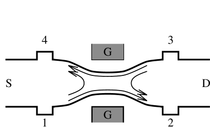
FIG. 1.: Schematic portrait of a point contact, in which the top and bottom edges of a Hall fluid are brought together by an electrostatically controlled gate (G), allowing for the tunneling of charge between the two edges. Here S and D denote source and drain, respectively.

For hierarchical FQHE states, at fillings $\nu\neq 1/q$, multiple edge modes are predicted[12], in some cases moving in both directions along a given edge. In the following we will focus for simplicity on the Laughlin sequence of states, and in particular on the most robust state at $\nu=1/3$.

Although FQHE edge modes at filling $\nu=1/3$, and a Luttinger liquid with $g=\nu$ are essentially equivalent, there are some subtle differences which must be kept in mind. Specifically, in the Luttinger liquid the fundamental (right moving) charge $e$ Fermion operator (the electron) is given from (6) by $\psi_{R}\sim e^{i(\theta+\phi)}$. This can be re-written in terms of the right and left moving Boson modes, $\phi_{R/L}=g\phi\pm\theta$, as $\psi_{R}\sim e^{i(2\phi_{R}+\phi_{L})}$. This operator thus adds charge $2/3$ into the right moving Boson mode, and $1/3$ into the left. In the FQHE, this corresponds to adding $2$ fractionally charged quasiparticles (charge $e/3$) to the top edge of the Hall bar, and $1$ to the bottom edge. But this is a non-local operator, and hence unphysical in the FQHE, whereas it is nice local operator in a quantum wire.

2 Inter-edge tunneling at a Point Contact

As discussed in Sections III and IV, the most remarkable property of a Luttinger liquid is the vanishing density of states for tunnelling electrons. To allow for intermode edge tunnelling in the FQHE, it is necessary to bring together the opposite edges of the Hall bar. This can be achieved by gating the electron gas, as depicted schematically in the Figure 1.

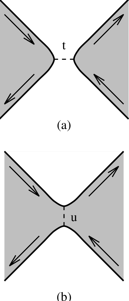
FIG. 2.: A quantum Hall point contact in the (a) weak tunneling limit and (b) the weak backscattering limit. The shaded regions represent the quantum Hall fluid with edge states depicted as lines with arrows. The dashed line represents a weak tunneling matrix element connecting the two edges.

Consider specifically, a gate which brings the opposite edge modes together at one point. This is equivalent to putting a single defect in an otherwise clean Luttinger liquid. In this geometry, charge can tunnel between the top and bottom edge modes, through the narrow strip of FQHE fluid (see Fig. 1). The appropriate term to add to the Hamiltonian is given in (22), and corresponds to the transfer of a fractionally charged Laughlin quasiparticle (charge $e^{*}=\nu e=e/3$) from top to bottom, with amplitude $u$. In a Luttinger liquid, this same perturbation corresponds to a weak $2k_{F}$ electron backscattering, with “backflow”.

Since $g=\nu<1$ this weak backscattering amplitude, $u$, grows at low temperatures, and the system crosses over into a large barrier regime, as discussed in Section IV. The large barrier limit corresponds to Figure 2a, in which the incident top edge mode is almost completely reflected. Weak tunnelling from left to right can be treated perturbatively, in the amplitude, $t_{0}$. In this case, it is an electron which is tunnelling, with charge $e$. As shown in Section IV A, (Eqn. (45)), this leads to a conductance which vanishes as a power of temperature,

$$G\propto t_{0}^{2}T^{(2/\nu)-2}\sim T^{4},$$ (82)

for $\nu=1/3$.

Fig. 3 shows data[27] for the conductance as a function of temperature through a point contact in an IQHE fluid at $\nu=1$ and a FQHE fluid at $\nu=1/3$.

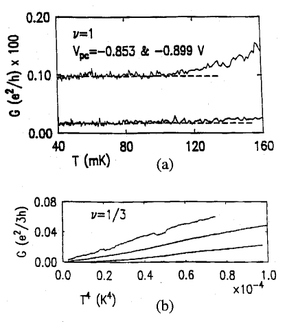
FIG. 3.: Conductance of a quantum point contact as a function of temperature for (a) $\nu=1$, and (b) $\nu=1/3$. Taken from Ref. [27].

The difference in behavior is remarkable. For $\nu=1$ the conductance approaches a constant at low temperatures, whereas for $\nu=1/3$ the conductance continues to decrease upon cooling. Moreover, the low temperature behavior for $\nu=1/3$ is consistent with the $T^{4}$ dependence predicted in (82). This data provides experimental evidence for the Luttinger liquid, a phase discussed theoretically over 30 years earlier.

In this same experiment, the conductance through the point contact was measured as a function of a gate voltage, controlling the pinch-off. The data in Fig. 4, shows a sequence of reproducible conductance peaks. A natural interpretation is that these are resonant tunnelling peaks, through a state localized in the vicinity of the point contact. As discussed in Section IV E, resonant tunnelling peaks are expected in a Luttinger liquid whenever the amplitude for the dominant backscattering process ($u_{1}$) is tuned to zero. In the FQHE, this process corresponds to tunnelling a single $e/3$ quasiparticle from the top to bottom edge. Since $\nu>1/4$, the higher order processes which involve multiple quasiparticle tunnelling are irrelevant. Thus, for a symmetric scattering potential, finding a resonance requires tuning only a single parameter, such as the gate potential.

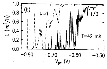
FIG. 4.: Two-terminal conductance as a function of gate voltage of a GaAs quantum Hall point contact taken at 42 mK. The two curves are taken at magnetic fields which correspond to $\nu=1$ and $\nu=1/3$ plateaus. Taken from Ref. [27].

Fig. 5 shows a scaling plot of one of the resonances for $\nu=1/3$ in Fig. 4 from the data of Webb et al. The widths of the resonances at several different temperatures have been rescaled by $T^{2/3}$, as suggested by (79). Since the peak heights were also weakly temperature dependent (and roughly one third of the quantized value $(1/3)e^{2}/h$) the amplitudes have also been normalized to have unit height at the peak. The temperature scaling of the peak widths is indeed very well fit by $T^{2/3}$. Also shown in Fig. 5 are quantum Monte Carlo data and an exact computation from Bethe Ansatz for the universal scaling function in (4.38). The agreement is striking. Although the experimental lineshape does drop somewhat faster in the tails, the shape is distinctly non Lorentzian with a tail decaying with a power close to that predicted by theory. It should be emphasized that the experimental data does not represent a “perfect resonance”, since the peak amplitude is dropping (slowly) upon cooling, rather than approaching the quantized value, $(1/3)e^{2}/h$. By varying an additional parameter besides the gate voltage (such as the magnetic field) though, it should be possible to find a perfect resonance for $\nu=1/3$.

FIG. 5.: Log-log scaling plot of the lineshape of resonances at different temperatures. The x axis is rescaled by $T^{2/3}$. The crosses represent experimental data of Ref. [27] at temperatures between $40mK$ and $140mK$. The squares are the results of the Monte Carlo simulation, and the solid line is the exact solution from Ref. [24].

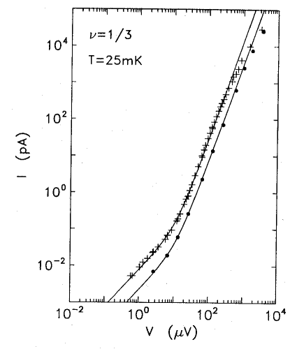
FIG. 6.: Current-voltage characteristics for tunneling from a bulk-doped $n+$ GaAs into the edge of a $\nu=1/3$ fractional quantum Hall fluid for two samples: Sample 1 at magnetic field $B=13.4$T (crosses), and sample 2 at $B=10.8$T (solid circles). The solid curves represent fits to the theory; the extracted values of the exponents for the two curves are $\alpha=2.7$ and $\alpha=2.6$ respectively. (Taken from Ref. [28].)

In a very recent experiment, Chang et. al.[28] have succeeded in tunnelling into a FQHE edge from a bulk metallic system. The 2DEG was exposed, in situ, by cleaving a bulk GaAs sample. A thin insulating barrier was grown onto the cleaved face. Heavily doped material was deposited on top of the insulating layer. The experiment measured the tunnelling conductance from the heavily doped “metal” through the insulating barrier into the FQHE edge. The tunnelling conductance from a Fermi liquid into a $g=\nu$ chiral Luttinger liquid, is predicted to vanish as, $G\sim T^{(1/\nu)-1}$. Since the DOS in a Fermi liquid is constant, this power is $1/2$ as large as for tunnelling between two $g=\nu$ chiral Luttinger liquids. Similarly, at zero temperature, the I-V curve is predicted to vary as $I\sim V^{1/\nu}$. Figure 6 shows data for the $I$-$V$ curve which is consistent with this power law.

B Coulomb blockade of strong tunneling

In this section we apply the mathematical tools developed for a 1d Luttinger liquid, to an apparently unrelated physical problem - namely the Coulomb blockade. Consider a conducting metallic grain (or “dot”) connected to an infinite lead by a junction, see Fig. (7a).

FIG. 7.: (a): Metallic grain connected to a lead by a channel (taken from Ref. [30]). The charge on the grain is controlled by the gate voltage, $V_{g}$, applied to an electrode which is coupled capacitively to the grain. (b): One-dimensional channel connecting the grain to the lead.

The grain is also coupled capacitively to another gate electrode. The electrostatic energy of the grain is

$$H_{Q}=\frac{(Q-eN)^{2}}{2C_{0}},$$ (83)

where $Q$ is the charge of the grain and $C_{0}$ is its capacitance. The parameter $N$ is proportional to the gate voltage $V_{g}$. Variation of the gate voltage $V_{g}$ changes the equilibrium charge of the grain. If the channel to the lead is almost depleted, and its conductance $G\to 0$, then the charge $Q$ can only take on discrete values $Q={{\cal N}}e$. The equilibrium charge $\langle Q\rangle$ should minimize the energy (83) within the set of integer ${\cal N}$, and therefore changes in a stepwise fashion with the gate voltage, $\langle Q\rangle={\rm Int}Ne$. On the other hand, if $G$ is large, one expects the grain charge to vary linearly with the gate voltage, $\langle Q\rangle=Ne$. Of interest is the behavior in the crossover region between these two limiting cases, as the conductance to the lead is varied.

This problem is non-trivial, because the electron-electron interaction term (83) must be treated non-perturbatively. As we shall see, if the junction is modelled as a single-mode channel with tunable reflection amplitude $r$, it is possible[29, 30] to apply the methods described in Section II. Indeed, using bosonization, Matveev[30] has shown that $\langle Q\rangle=Ne$ at $r=0$, and found analytically the function $q(N)\equiv\langle Q\rangle-Ne$ for weak reflection. (Here and after, $\langle\dots\rangle$ denotes a ground-state average.) The average charge is directly related to the ground state energy, $q(N)=-(C_{0}/e)\partial E/\partial N$. Below we follow closely the line of arguments presented in Ref. [30].

To find the ground state energy $E$, we need to supplement the Hamiltonian (83) by a part describing non-interacting electrons. For the case of a grain with size $L$ large compared to the Bohr radius, $a_{B}=\hbar^{2}/me^{2}$, this can be simplified. If the motion within the grain is chaotic, then the dwelling time for an electron entering the grain through a single-mode channel is $\tau_{d}\sim\delta^{-1}$, where $\delta$ is the electron level spacing in the grain. On the other hand, the quantum charge fluctuations which destroy the discreteness of $\langle Q\rangle$ occur on the time scale $\tau_{q}\sim 1/E_{C}$, where $E_{C}\sim e^{2}/C_{0}$ is the single-electron charging energy. The latter time scale is relatively short, $\tau_{q}/\tau_{d}\sim a_{B}/L\ll 1$ (the estimate is performed for a two-dimensional grain). Over this time, electrons participating in the charge fluctuations (i.e., those that pass through the channel) do not get back into the channel after “exploring” the grain. It means that we need to add to Eq. (83) a Hamiltonian describing only the electrons moving through a one-dimensional channel. In the absense of a barrier within the channel, this Hamiltonian is

$$H_{0}=iv_{F}\int dx\left[\psi_{R}^{{\dagger}}(x)\partial_{x}\psi_{R}(x)-\psi_{L}^{{\dagger}}(x)\partial_{x}\psi_{L}(x)\right],$$ (84)

where $\psi_{R}^{{\dagger}}(x)$ and $\psi_{L}^{{\dagger}}(x)$ are the creation operators for right- and left-movers, respectively. We have used here a linearized electron spectrum, since the energy scale $E_{C}$ is much smaller than the Fermi energy, $E_{C}/E_{F}\sim(a_{B}/L)(k_{F}a_{B})^{-2}\ll 1$.

The definition of the charge operator $Q$ in Eq. (83) depends on where we “draw” the boundary between the channel and the grain. This arbitrariness in convention only affects the phase of the oscillations of $q(N)$. But this phase does not carry any physical meaning, provided the gate voltage is small enough not to deplete the grain entirely. Therefore, $Q$ can be viewed as the charge passed e.g. through the middle ($x=0$) of the channel, Fig. (7b) into the dot,

$$Q=e\int_{0}^{\infty}dx\left[\psi_{R}^{{\dagger}}(x)\psi_{R}(x)+\psi_{L}^{{\dagger}}(x)\psi_{L}(x)\right].$$ (85)

Now, with the help of Eq. (8), we can bosonize the Hamiltonian (84), which gives Eq. (4) with $g=1$,

$$H_{0}={v_{F}\over{2\pi}}[(\partial_{x}\phi)^{2}+(\partial_{x}\theta)^{2}].$$ (86)

Bosonization of the interaction part (83) is also straightforward, after we put $\psi_{R}^{{\dagger}}(x)\psi_{R}(x)+\psi_{L}^{{\dagger}}(x)\psi_{L}(x)\to-\partial_{x}\theta(x)/\pi$ into (85),

$$H_{C}=E_{C}\left[\frac{1}{\pi}\theta(0)-N\right]^{2},\quad E_{C}=\frac{e^{2}}{2C}.$$ (87)

In the absence of a barrier in the channel, it is easy to show that $q(N)=0$. Indeed, after the transformation

$$\theta(x)\to\theta(x)+\pi N,$$ (88)

the Hamiltonian $H_{0}+H_{C}$ does not depend on $N$; there is no Coulomb blockade at $r=0$. The ground state energy starts to depend on $N$, if a barrier causes backscattering in the channel. The corresponding Hamiltonian (cf Eq. (21)) in the boson variables is

$$H_{\rm imp}=-\frac{u}{\pi v_{F}}D\cos[2\theta(0)],$$ (89)

where $u$ is the $2k_{F}$–component of the scattering potential, and $D$ is a high energy cut-off. The transformation (88), makes evident the periodic dependence of the full Hamiltonian, $H_{0}+H_{\rm imp}+H_{C}$, on $N$.

To find the correction to the ground state energy to first order in $|r|$, denoted $E_{1}$y, the perturbation (89) must be averaged in the ground state of the Hamiltonian $H_{0}+H_{C}$, Eqs. (86), (87). It then follows directly from Eqs. (86), (87) and (88), that $E_{1}\propto\cos(2\pi N)$. The proportionality coefficient can be estimated with the help of the RG equation (51). In the absence of the local interaction (87), the renormalization (51) is valid for all energy scales and can be taken to the limit $\ell\to\infty$, which results in a vanishing effective scattering potential, $E_{1}=0$. With a finite $E_{C}$, the renormalization should be stopped at $\exp(-\ell)\sim E_{C}/D$, which at $g=1$ leads to $E_{1}=-{\rm const}\cdot(u/v_{F})E_{C}\cos 2\pi N$. To leading order in the backscattering, $|r|=u/v_{F}$, so that

$$E_{1}=-{\rm const}\cdot|r|E_{C}\cos 2\pi N.$$ (90)

An exact result for $E_{1}$ obtained[30] in the framework of the Debye-Waller theory for the quadratic Hamiltonian $H_{0}+H_{C}$, yields ${\rm const}=e^{\bf C}/\pi^{2}$, with ${\bf C}\approx 0.5772$ being Euler’s constant. Finally,

$$\frac{q(N)}{e}=-\frac{e^{\bf C}}{\pi}|r|\sin 2\pi N.$$ (91)

VI Conclusion

In this paper we have reviewed recent theoretical results for transport in a one-dimensional (1d) Luttinger liquid. For simplicity, we have ignored electron spin, and focussed exclusively on the case of a single-mode. Moreover, we have considered only the effects of a single (or perhaps several) spatially localized impurities. Even with these restrictions, the predicted transport behavior is qualitatively different than for a non-interacting electron gas. Specifically, for repulsive interactions, even a weak impurity potential causes complete backscattering, and the conductance vanishes completely at zero temperature. This can be understood in terms of the vanishing density of states, to tunnel an electron throught the barrier from one semi-infinite Luttinger liquid to another. At finite temperature the tunnelling electron has finite energy, and the conductance is non-zero, varying as a power of temperature. The precise power law depends on the dimensionless parameter (conductance) $g$ which characterizes the Luttinger liquid.

For a very weak barrier, at elevated temperatures, the backscattering is weak, but grows rapidly with cooling. This growth can be understood physically in terms of the fact that the discrete backscattered charge in this limit, is less than the electron charge $e$, but rather given by $ge$ with $g<1$ for a repulsively interacting electron gas (see Eqn. (2.22)). For inter-edge tunnelling in the fractional quantum Hall effect, this process corresponds to the backscattering of a Laughlin quasiparticle (with $g=\nu=1/3$, say), but such fractionally charged excitations are in fact a generic property of the 1d Luttinger liquid, and should be present, for example, in narrow quantum wires. The fractional charge might be directly measureable via shot-noise experiments through a single impurity.

The transport behavior in a 1d Luttinger liquids is of course much richer once one relaxes the restrictions of a single impurity and a single channel. The case of a single channel with many impurities has been considered by a number of authors[31]. In the absence of electron interactions, all states are localized in 1d, and the system is an insulator. With repulsive interactions, localization effects are enhanced, and the system is insulating, even though the notion of single particle localized eigenstates is no longer operative. However, for spinless electrons with sufficiently strong attractive interactions, the system is predicted to undergo an insulator-to-metal transition. In the metallic phase, the conductivity is predicted to diverge as a power law of temperature (with a variable power greater than one), in contrast to a normal 3d metal, in which there is a finite residual resistivity at $T=0$. While the electron interaction in a quantum wire is clearly repulsive, a long skinny gate across a fractional quantum Hall fluid at, e.g., filling $\nu=1/3$, creates a system which is isomorphic to a (spinless) 1d electron gas with strong attractive interactions[32]. By varying the gate potential along such a line junction, it should be possible to tune through this 1d localization transition.

For a real one-channel quantum wire, it is of course necessary to take into account the spin of the electron[22, 33]. The method of bosonization can readily accomodate the spin degree of freedom. The spinful interacting electron gas has two modes, one which carries the charge and the other the spin[3, 7]. These two modes will generally propagate at different velocities, a phenomena known as charge/spin separation. The effects of impurity scattering on the spinful electron gas are qualitatively similar to that without spin. Specifically, with repulsive interactions, a single impurity will typically be sufficient to completely backscatter both the charge and spin modes. The conductance will be driven to zero as a power law of temperature, with possible logarithmic corrections. Resonant tunnelling is also possible for a spinful electron gas, but can occur in several different guises, depending on the charge and spin state of the localized state.

In a wider quantum wire, several transverse modes will co-exist at the Fermi energy. This can also be treated with bosonization. Generally, associated with each channel is one gapless charge mode and one gapless spin mode. The tunnelling density of states to add an electron, will generally still be singular, as for a single channel, but the associated exponents become smaller as the number of channels increase[18, 34]. Multiple channels are also present at the edges of hierarchical fractional quantum hall states[35], such as at filling $\nu=2/3$ . Multi-component models are also necessary to treat charge fluctuations under the Coulomb blockade conditions (Section V B) in the realistic case of electrons with a spin degree of freedom. Indeed, a recent theory of Coulomb blockade effects for coupled quantum dots[36], has yielded predictions which are in quantitative accord with experiment[37].

VII Acknowledgements

We have both benefitted from extensive interactions with numerous friends and collaborators over the past years. We are particurly indebted to Igor Aleiner, Harold Baranger, Albert Chang, Steve Girvin, Bertrand Halperin, Charlie Kane, Anatoly Larkin, Patrick Lee, Hsiuhau Lin, Andreas Ludwig, Allan MacDonald, Konstantin Matveev, Kyungson Moon, Joe Polchinski, Igor Ruzin, Boris Shklovskii, M. Stone, Richard Webb and Hangmo Yi. We gratefully acknowledge the National Science Foundation for support under grants DMR-9400142, PHY89-04035 and DMR-9528578 (University of California at Santa Barbara), and No. DMR-9423244 (University of Minnesota).

REFERENCES

- [1] “Methods of Quantum field theory in statistical physics”, by A.A. Abrikosov, L.P. Gorkov and I.E. Dzyaloshinski, (Dover, New York, 1963).
- [2] See R. Shankar, Rev. Mod. Phys. 66, 129 (1994) and references therein.
- [3] For a review, see e.g., J. Solyom, Adv. Phys. 28, 201 (1979).
- [4] S. Tomonaga, Prog. Theor. Phys. (Kyoto) 5, 544 (1950).
- [5] J.M. Luttinger J. Math. Phys. N.Y. 4, 1154 (1963).
- [6] F.D.M. Haldane, J. Phys. C14, 2585 (1981); Phys. Rev. Lett. 47, 1840 (1981).
- [7] See, e.g., G.D. Mahan, Many-Particle Physics, 2nd ed. (Plenum Press, New York, 1990), section 4.4.
- [8] D. C. Mattis, Phys. Rev. Lett. 32, 714 (1974).
- [9] A. Luther and I. Peschel, Phys. Rev. Lett. 32, 992 (1974).
- [10] A. Luther and V. J. Emery, Phys. Rev. Lett. 33, 589 (1974).
- [11] B. I. Halperin, Phys. Rev. B 25, 2185 (1982).
- [12] X. G. Wen, Phys. Rev. B 43, 11025 (1991); Phys. Rev. Lett. 64, 2206 (1990); Phys. Rev. B 44, 5708 (1991).
- [13] L. I. Glazman, G. B. Lesovik, D. E. Khmel’nitskii, and R. I. Shekhter, Pis’ma Zh. Eksp. Teor. Fiz. 48, 239 (1988) [JETP Lett. 48, 238 (1988)].
- [14] R. Landauer, IBM J. Res. Dev. 1, 223 (1957).
- [15] I.E. Dzyaloshinskii, A.I. Larkin, ZhETF 63, 411 (1973).
- [16] D.L. Maslov, M. Stone, Phys. Rev. B52, 5539 (1995); I. Safi, H.J. Schulz, Physical Review B 52, 17040 (1995); V.V. Ponomarenko Physical Review B52, 8666 (1995).
- [17] C. L. Kane and M. P. A. Fisher, Phys. Rev. Lett. 68, 1220 (1992).
- [18] K.A. Matveev, L.I. Glazman, Physics B, 189, 266 (1993).
- [19] C. L. Kane and M. P. A. Fisher, Phys. Rev. Lett. 72, 724 (1994).
- [20] L.I. Glazman, I.M. Ruzin, B.I. Shklovskii, Phys. Rev. B 45, 8454 (1992).
- [21] A similar logarithmic divergency with the system size at was found in the problem of the charge density wave tunneling, see A.I. Larkin, P.A. Lee, Phys. Rev., B17, 1596 (1978).
- [22] K.A. Matveev, D. Yue, L.I. Glazman, Phys. Rev. Lett., 71, 3351 (1993) ; D. Yue, K.A. Matveev, L.I. Glazman, Phys. Rev. B 49, 1966 (1994).
- [23] K. Moon, H. Yi, C.L. Kane, S.M. Girvin, M.P.A. Fisher, Phys. Rev. Lett. 71, 4381 (1993).
- [24] P. Fendley, A.W.W. Ludwig, H. Saleur, Phys. Rev. Lett. 74, 3005 (1995).
- [25] S. Tarucha, T. Honda, T. Saku, Solid State Commun. 94, 413 (1995).
- [26] A. Yacoby, H.L. Stormer, L.N. Pfeiffer, K.W. West (unpublished).
- [27] F.P. Milliken, C.P. Umbach, R.A.Webb, Solid State Commun. 97, 309 (1996).
- [28] A.M. Chang, L.N. Pfeiffer, K.W. West, Phys. Rev. Lett. 77, 2538 (1996).
- [29] K. Flensberg, Phys. Rev. B 48, 11156 (1993); Physica B 203, 433 (1994).
- [30] K.A. Matveev, Phys. Rev. B 51, 1743 (1994); Physica B 203, 404, (1994).
- [31] See T. Giamarchi and H. Schulz, Phys. Rev. B37, 325 (1988), and references therein.
- [32] S. Renn and D.P. Arovas, Phys. Rev. B51, 16832 (1995).
- [33] C.L. Kane and M.P.A. Fisher, Phys. Rev. B 46, 15233 (1992).
- [34] K.A. Matveev, L.I. Glazman, Phys. Rev. Lett., 70, 990 (1993).
- [35] C.L. Kane, M.P.A. Fisher, J. Polchinski, Phys. Rev. Lett., 72, 4129 (1994); C.L. Kane and M.P.A. Fisher, Phys. Rev. B 51, 13449 (1995).
- [36] K.A. Matveev, L.I. Glazman, H.U. Baranger, Phys. Rev. B 53, 1034 (1996); J.M. Golden, B.I. Halperin, Phys. Rev. B 53, 3893 (1996).
- [37] F.R. Waugh, M.J. Berry, D.J. Mar, R.M. Westervelt, K.L. Campman, A.C. Gossard, Phys. Rev. Lett. 75, 705 (1995).