Improved Magnetic Information Storage using Return–Point Memory

Abstract

The traditional magnetic storage mechanisms (both analog and digital) apply an external field signal $H(t)$ to a hysteretic magnetic material, and read the remanent magnetization $M(t)$, which is (roughly) proportional to $H(t)$. We propose a new analog method of recovering the signal from the magnetic material, making use of the shape of the hysteresis loop $M(H)$. The field $H$, “stored” in a region with $N$ domains or particles, can be recovered with fluctuations of order $1/N$ using the new method — much superior to the $1/\sqrt{N}$ fluctuations in traditional analog storage.

PACS numbers: 85.70.Li, 75.60.Ej, 85.70.Ay, 75.60.-d

A Introduction

How can one best store a song on a magnetic tape? The traditional analog method converts the sound signal into a magnetic field $H(t)$, and then uses it to magnetize the tape, being pulled at a velocity $v$. The remanent magnetization $M$ (the magnetization left on the tape after the field has dropped to zero) is roughly linear in $H$:

$$M(x)=M(vt)=C_{1}\,H(t)+C_{2}\,H^{2}(t)+\eta(x).$$ (1)

Here $C_{2}$ represents the nonlinearity of the remanent magnetization at high fields (when recording, one turns down the gain until the needle during the loudest sections stops moving into the red), and $\eta$ represents noise (one turns up the gain as far as possible so quiet portions don’t hiss). (Actually, there are nonlinearities between the remanent magnetization and the signal $H(t)$ for low fields as well (not shown in equation (1)). When real magnetic tapes are recorded, the signal $H(t)$ is convolved with a high-frequency, large amplitude signal [1, 2, 3, 4] in order to remove these distortions (ac–biasing). This however does not affect the new method for analog storage that we propose.)

Two other excellent methods have been developed to cope with the noise and nonlinearity in the remanent magnetization. (There are other sources of noise in a magnetic recording and reading process, e.g., interference, electronic noise, and head noise [3, 5, 6]. In this paper, we will address only the noise relevant to the magnetic material: the magnetic noise.) Dolby noise reduction does a nonlinear transformation of H(t) to boost quiet sections and dampen loud sections: the inverse transformation is applied at playback. Digital recordings are even more effective. The signal can be (linearly and accurately) encoded as a stream of bits, and these bits can be recorded and reproduced without noise or distortion.

How does the analog method compare to digital recording, in terms of the amount of information that one can store on a given piece of magnetic tape? One important[1, 3, 6] source of noise is the lumpiness of the irreversable magnetization changes in the material. Magnetic tapes are often made up of single-domain particles; if the field is strong enough, some particles will rotate their magnetizations to the crystallographic axis closest to the direction of the field [7]. Other materials with large domains will magnetize through the depinning of sections of their domain walls, which (roughly) jump from one pinning center to another. For our purposes, these details aren’t crucial — we mostly care about the number $N$ of these pinning centers or particles. We will refer to these lumps, imprecisely, as domains.

Having more, smaller domains leads to a higher information density. Averaging over $N$ domains will reduce the fluctuation in the average magnetization by a factor of $1/\sqrt{N}$ (presuming the interactions between domains are not important). Thus, the number of different values of $H$ that can be distinguished in the remanent magnetization scales like $\sqrt{N}$. If we subdivide the slice into $Q$ portions, and magnetize each portion separately, we can store $\sqrt{N/Q}^{Q}$ different signals. Optimizing, we find $Q=N/e$, and we store $e^{N/2\,e}$ distinguishable signals. This is precisely what makes the binary “digital” recording so effective: $2^{Q}$ strings of $Q$ bits are stored, and our formula suggests that four domains can store one bit ($Q=N/4$). Of course, substantial error correction would be needed in order to keep the accuracy high at this scale!

There are times when one is stuck with an analog signal. Important recordings have been made with these outdated methods (Beatles’ masters) and potentially one might want to reconstruct signals imposed by natural processes (reconstructing the stress history of a plastically deformed material). We show here that one can do substantially better than the traditional analog retrieval, by using the portion of the magnetization curve $M(H)$ near the applied field $H_{signal}$ (e.g., by the tape head during recording), rather than just the remanent magnetization at zero field $M(0)$. We discuss the advantages within the context of two models: the Preisach[8, 9] model of non-interacting hysteretic domains (which despite its simplistic assumptions is a standard tool[10] in the engineering community), and the zero–temperature random–field Ising model (RFIM) [11, 12] (a more realistic model incorporating nearest-neighbor couplings between domains with different threshold fields). In the end, we improve our resolution by $\sqrt{N}$ (from the $1/\sqrt{N}$ resolution of the remanent magnetization to $1/N$), which for a typical slice of magnetic tape with $N=10^{6}$ domains per wavelength (see conclusion) produces a large improvement in fidelity. Our method also suffers much less from nonlinearity: although the fidelity decreases at large magnetizations, the signature tracks the applied field directly. There is a drawback to our new method though: by measuring the response curve, the original signal is necessarily erased.

We should mention another method for dealing with the random noise in magnetic films that has been developed recently [13] by Des Mapps of Plymouth University in England. Instead of the usual two heads used in recording (one for demagnetizing the magnetic material and the other to record the signal), a third head is added, which reads the signal right after it has been recorded, and sends it to a computer for analysis. Since the computer “knows” what the initial signal was, it can adjust for the inherent noise in the magnetic material, record the now “modulated” signal, and leave a signature of what it has done. This provides the information to the “reading” head of how to compensate, during the reading process. Similar techniques have been independently developed by Indeck and Muller from Washington University in St. Louis [13].

B Hysteresis Loops, Subloops, Kinks, and Return–Point Memory

We review briefly the various kinds of $M(H)$ hysteresis curves relevant to our discussion. (There are many different curves, of course, since the response depends on the magnetic history of the material.) A ferromagnetic material has the property that its magnetization $M$ lags behind the external magnetic field $H$, as the field is changed (fig. 1). This is called hysteresis (which means to lag or fall behind). The largest magnetization the material can have (by aligning all the magnetic domains in the direction of the external field $H$) is called the saturation magnetization $M_{S}$. When the field is switched off, the remaining magnetization is the remanent magnetization $M_{R}$, while the field necessary to bring the magnetization to zero is called the coercivity $H_{C}$. Variations in the values of these properties in different ferromagnets make magnetic materials useful for different applications. For example, magnetic recording materials have high remanence and coercivity to prevent unwanted demagnetization [7]. Therefore, magnetic materials used in recording will in general have “square” hysteresis loops. By sweeping from very small to very large magnetic fields, one explores this saturated, “outer” hysteresis loop $M_{outer}^{\pm}$ (also called the major hysteresis loop): any other field history will typically be discussed in terms of subloops (or minor hysteresis loops) (see fig. 1).

FIG. 1.: Magnetization $M$ of a ferromagnet as a function of the external field $H$. The hysteresis curve appears due to a lag between the magnetization and the field. $M_{S}$ denotes the saturation magnetization, $M_{R}$ the remanent magnetization, and $H_{C}$ the coercivity (see text). The subloop $a\rightarrow b\rightarrow e\rightarrow a$ shows the return–point memory. The system comes back to the same state $a$, as the external field is switched off and then back on.

Before recording, the magnetic tape is demagnetized. This involves imposing a slowly decaying, oscillatory field $H(t)$ which leaves the material in a well-defined, reproducible state with no remanent magnetization (up to the noise). Analog recording takes us from this particular demagnetized state to a magnetized state under an external field $H_{signal}$: in real recording, this is done by adding an oscillating field to the signal (see introduction), but initially we will consider a monotonically increasing field, leading to an increasing magnetization $M_{imprint}(H)$. Releasing the external field, the magnetization $M_{relax}$ again drops, but to a non-zero remanent $M_{R}^{signal}$ (figure 2). Measuring $M_{R}^{signal}$ gives information about $H_{signal}$.

We will also be interested in $M_{measure}(H)$ curve, formed by starting from the magnetized state $M_{R}^{signal}$ and raising the field again. As one sees from figure 2, as the external field is decreased from the original signal $H_{signal}$ and then increased again, the magnetization forms a subloop. As the external field passes $H_{signal}$, there will be very generally a kink in the $M_{measure}(H)$ curve (figure 2). This follows in a direct way, for example, for models exhibiting return point memory [14] (also known as wiping out [9]).

FIG. 2.: The external field is increased to $H_{signal}$ and then decreased to zero (dashed curve). In the traditional analog storage, the information is stored in the remanent magnetization $M_{R}^{signal}$. In the new method, which uses the return–point memory property, the information is stored in the field $H_{signal}$ itself, read by increasing the external field from zero and finding a “kink” in the $M$–$H$ curve (solid curve).

For these systems, the subloop closes exactly: the system returns at $H_{signal}$ to precisely the same state it was in at the peak of its recording field (wiping out all information about the excursion to lower fields). The curve $M_{measure}(H)$ above $H_{signal}$ thus necessarily extends smoothly the original curve $M_{imprint}(H)$, while below $H_{signal}$ it disagrees with $M_{imprint}$: hence it must have a non-analyticity at $H_{signal}$. Magnetic recording materials often wipe out rather well: decreasing the field from $H_{signal}$ (and hence repeating the loop) will reproduce the same subloop (including even the noise) to a good extent[16]. On the other hand, magnetic materials — especially those like spin-glasses with important antiferromagnetic couplings — can exhibit “reptation”, where repeated cycles lead to a slow drift in magnetization[17]. Many other systems (e.g. martensites prepared with parallel twin boundaries [18], helium capillary condensing in a porous material [19], and superconductors in external magnetic fields [20]) can exhibit the return–point memory to various extents; see the work by Amengual et al. [18] for an experiment reproducing incredible fine structure within repeated loops. Reference [11] discusses three conditions [14] (partial ordering, no passing, and adiabaticity) which suffice to produce a perfect return-point memory. The models studied here possess these properties: antiferromagnetic couplings violate “no passing”.

For the purposes of this paper, the kink in $M_{measured}(H)$ is easily explained. As the field is raised a second time, the domains which flipped upon the first rise during imprinting and which did not flip back upon relaxing are not active. When $H$ crosses $H_{signal}$, new, “virgin” domains are explored: more domains will flip per unit field, leading to a discontinuity in the slope. It is precisely this slope discontinuity in the magnetization curve which we propose to use in information storage. Since the slope discontinuity is at $H_{signal}$, we are saved from the nonlinearity and distortion which occurs with only measuring the remanent magnetization. We will see in the next section that we also suppress the noise greatly.

C The Preisach and Random Field Ising Models

The comparison between the “traditional” magnetic analog storage method, in which the magnetization carries the information, with the new method where the whole hysteresis loop is retrieved, and the information is stored directly in the magnetic field, is done using the Preisach and random field Ising models. The Preisach model [8, 9] consists of a system of independent domains, each with an upper field $H_{u}$ and a lower field $H_{d}$, at which the domain changes sign (or direction). Each domain therefore has its own square hysteresis loop (see figure 3), and the superposition of all these loops gives a hysteresis loop as in figure 1. In general, the upper and lower fields are not equal and opposite, but the magnetization per domain $m_{0}$ is assumed constant. The Preisach model has the necessary properties for its hysteresis loop to exhibit return–point memory and is quite useful because of its simplicity, but since there are no interactions between the domains, the modeling of real systems is more limited. The random field Ising model [11, 12], on the other hand, includes nearest neighbor interactions.

FIG. 3.: Hysteresis loop for one domain in the Preisach model. The field at which the domain flips up is $H_{u}$ and the field at which it flips down is $H_{d}$. A superposition of many such domain hysteresis gives a hysteresis curve as in figure 1.

We first review the elements of the Preisach model that we will need. To calculate the magnetization in the Preisach model, a weight function $\rho(H_{d},H_{u})$ ($H_{u}\geq H_{d}$) needs to be defined. $\rho$ has the units of magnetization per unit field squared. For systems with time–reversal symmetry, $\rho$ is symmetric around the line $H_{u}=H_{d}$ in the $(H_{d},H_{u})$ plane [8, 9] (see figure 4). If all the domains are pointing down, and we increase the external field from a large negative value to $H_{signal}$ in figure 1, the domains whose field $H_{u}$ fall in the shaded area of figure 4 will flip up. The magnetization of the system is then given by:

$$M=\int\!\!\int_{U}\rho(H_{d},H_{u})\ dH_{u}dH_{d}-\int\!\!\int_{D}\rho(H_{d},H_{u})\ dH_{u}dH_{d}$$ (2)

where the first integration is over the area where the domains are pointing up (U), and the second is over the area where the domains are pointing down (D). If the system follows the path depicted in figure 1 (from a large negative field to $H_{signal}$ to $H_{b}$ to $H_{e}$), we obtain a “step” of flipped spins in the $(H_{d},H_{u})$ plane (figures 5(a,b)). (Several subloops would give a “staircase”.) The magnetization is again obtained using equation (2).

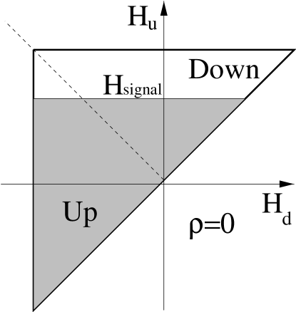
FIG. 4.: The triangular region is the region in $(H_{d},H_{u})$ space where the weighting function $\rho$ is defined (outside of it, $\rho=0$). The shape of this region is in practice much more general, and depends on the properties of the magnetic material [21], but the region is usually symmetric around the $H_{u}=-H_{d}$ line. As the field is raised from a large negative value of the field to $H_{signal}$ (see fig. 1), the domains in the shaded region flip up. The magnetization is obtained from equation (2).

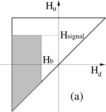
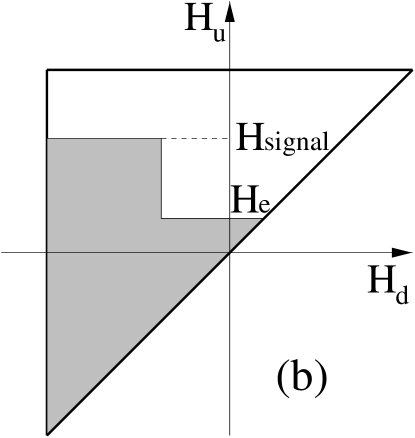
FIG. 5.: (a) The $(H_{d},H_{u})$ plane after the field has been increased to $H_{signal}$ (from a large negative value), and then decreased to a value $H_{b}$ (see fig. 1). The shaded area corresponds to spins (domains) that have flipped (and not flipped back). (b) The field has now been increased to a value $H_{e}$. More spins have flipped, and we find a “step” in the Preisach plane. Several subloops would give a “staircase” (see for example figure 6b).

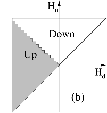
FIG. 6.: (a) The ac magnetic field used to demagnetize the tape before storing the analog signal. (b) The demagnetization process in the $(H_{d},H_{u})$ plane. The “staircase” occurs after taking the system through smaller and smaller loops.

The zero–temperature random field Ising model has the following Hamiltonian [11, 12]:

$${\cal H}=-\sum_{<i,j>}J_{ij}s_{i}s_{j}-\sum_{i}(H+h_{i})s_{i}$$ (3)

where $J_{ij}$ is the nearest neighbor interaction between spins (domains) $s_{i}$ and $s_{j}$ (we set all $J_{ij}=J=1$), $H$ is the uniform external magnetic field, and $h_{i}$ is a random field at site $s_{i}$ given by a Gaussian probability distribution. The dynamics is such that a spin $s_{i}$ will flip when its “effective” field $h^{ef\!f}_{i}=J\sum_{j}s_{j}+H+h_{i}$ changes sign. A spin that flips can trigger other spins to flip due to the interaction between nearest neighbors: avalanches of spins are possible. This model gives rise to a hysteresis loop and has the return–point memory property [11].

We use the Preisach model with a constant magnetization $m_{0}$ per domain, to calculate the relative fluctuations in the signal for the “traditional” analog magnetic storage and the new method. The weight function $\rho$ can be written as $N\,m_{0}\,\tilde{\rho}$ with $\tilde{\rho}$ being the probability distribution for the domains in the $(H_{d},H_{u})$ plane. We also simulate magnetic systems of different sizes using the random field Ising model. These are then compared to the analytical results.

D Traditional Analog Magnetic Storage

In the traditional analog recording, the tape (system) is first demagnetized [21] by applying a strong ac field which is gradually reduced to zero (figure 6a). In figure 6b, the demagnetization process is show in the $(H_{d},H_{u})$ plane for the Preisach model. In the limit of a very fine “staircase” (the ac field needs to drop off very slowly), the magnetization of the system become zero.

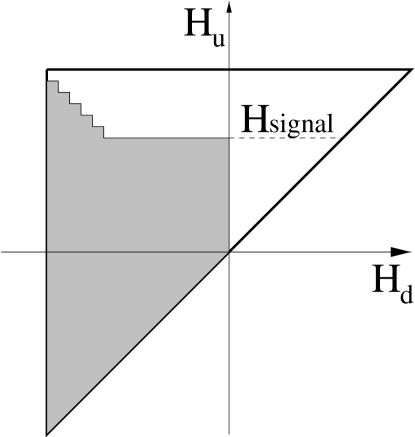
FIG. 7.: Recording the signal as the remanent magnetization $M_{R}^{signal}$, starting from a demagnetized system (in the Preisach Plane). The shaded area represents the system at $M=M_{R}^{signal}$ and $H=0$. The average value of the remanent magnetization $M_{R}^{signal}$ can be calculated using equation (2).

The tape is now ready to be recorded. The external field is raised from zero until a value $H_{signal}$ (below the saturation value of the system), and then switched off. At zero field, the tape stays magnetized with the remanent magnetization $M_{R}^{signal}$ (figure 2). The magnetization $M_{R}^{signal}$ can be calculated from figure 7 using equation (2). However, we can calculate the magnetization differently if we notice that the probability for a domain to be pointing up is given by:

$$p=\int\!\!\int_{U}\tilde{\rho}(H_{d},H_{u})\,dH_{u}\,dH_{d}$$ (4)

where the integration is over the shaded region in figure 7. For $N$ independent domains, the probability $P(n;N,p)$ for observing $n$ up domains out of a total of $N$ is given by the binomial distribution [22]:

$$P(n;N,p)={N!\over{n!\,(N-n)!}}\,p^{n}\,(1-p)^{N-n}$$ (5)

Then, the average number of domains that are up is $Np$, with a root mean square (rms) of $\sqrt{Np\,(1-p)}$.

Since we are interested in the measurement of the magnetization, the average magnetization will be $(2Np-N)\,m_{0}$. If we take the rms to be our measure of the fluctuation around the average, then the fluctuation relative to the saturation magnetization is:

$${|\Delta M_{R}^{signal}|\over|M_{S}|}={m_{0}\,2\sqrt{N\,p(1-p)}\over N\,m_{0}}={2\,\sqrt{p(1-p)}\over\sqrt{N}}$$ (6)

where $p$ has a value between zero and one. The size $1/\sqrt{N}$ of this relative fluctuation limits the amount of information that can be stored using the traditional analog magnetic storage, in a system with $N$ domains.

E New Method for Analog Magnetic Storage

With the new method for analog storage, the information is stored in the value of the external field $H_{signal}$ at which the kink in the hysteresis occurs. Similarly to the traditional analog storage, we have a limitation on how well the information can be retrieved given by a value proportional to $\Delta H_{signal}/H_{C}$, where $\Delta H_{signal}$ gives the fluctuation around the value $H_{signal}$, and $H_{C}$ is the coercivity.

As before, we start with the tape (system) demagnetized, and increase the field up to a value $H_{signal}$, smaller than the saturation field. The external field is then switched off (fig. 2). The system will be magnetized with a remanent magnetization $M_{R}^{signal}$. When the information needs to be recovered, instead of “reading off” the value of the remanent magnetization $M_{R}^{signal}$, the external field is increased until a kink in the $M$–$H$ curve is found. If the system exhibits the return–point memory property, the field at which the kink occurs is $H_{signal}$. In the $(H_{d},H_{u})$ plane (figure 8), the kink is seen as a discontinuous increase in the number of domains flipped as the field is increased past $H_{signal}$. (If the original signal is ac–biased, as in audio signals, there is a discontinuity in the Preisach plane [4] at a field shifted up from $H_{signal}$ by about the amplitude of the ac–bias (see figures 9(a,b). The retrieval of this value is otherwise analogous to the presentation that follows.)

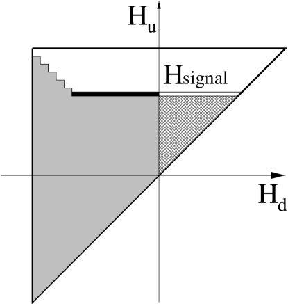
FIG. 8.: Storage of information in the field $H_{signal}$ using the return–point memory effect, as seen in the Preisach plane. The shaded area represents the system at $M=M_{R}^{signal}$ and $H=0$. As the field is increased, spins in the cross–hatched region flip up. At $H_{signal}$ there is a discontinuity in the number of spins flipping per unit field. This appears as a kink in the $M$–$H$ curve. The integral of the weight function $\rho$ over the black horizontal strip is ($f^{(2)}-f^{(1)}$), and over the white strip is $f^{(1)}$.

To observe the kink, we can take the derivative of the hysteresis curve with respect to the field $H$ and observe the discontinuity. In general the data will need to be smoothed over some range $\Delta H$, which will help in finding the discontinuity in the slope, but will introduce fluctuations around $H_{signal}$ of the order of $\Delta H$. The discontinuity in the slope can be observed if the difference between the number of domains that flip in a range $\Delta H$, below and above $H_{signal}$, is larger than the standard deviation in the number of domains flipped in $\Delta H$ above $H_{signal}$:

$$\Delta N_{\uparrow}^{(2)}-\Delta N_{\uparrow}^{(1)}>\sqrt{Np^{(2)}(1-p^{(2)})}$$ (7)

where the superscripts $(1)$ and $(2)$ indicate measurements below and above $H_{signal}$ respectively, and $p^{(2)}$ is the probability that a domain flips from down to up in a range $\Delta H$, just above $H_{signal}$. (In general we should require that the difference be larger than the fluctuations just above and below $H_{signal}$, but since the fluctuations below $H_{signal}$ are smaller, we can use equation (7).) Note that $Np^{(2)}=\Delta N_{\uparrow}^{(2)}$. If the interval $\Delta H$ is small enough, that the slope $f=dM/dH$ of the $M$–$H$ curve can be considered close to constant, we have:

$${(f^{(2)}-f^{(1)})\over m_{0}}\,\Delta H>\sqrt{{f^{(2)}\over m_{0}}\,\Delta H\,(1-p^{(2)})}$$ (8)

Thus the uncertainty in the measured $H_{signal}$ is:

$$\Delta H_{signal}\sim\Delta H>{m_{0}\,f^{(2)}\,(1-p^{(2)})\over(f^{(2)}-f^{(1)})^{2}}$$ (9)

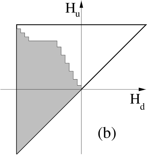
FIG. 9.: (a) Magnetic field as “seen” by a magnetic tape moving past a recording head with an ac–biased field superimposed on a constant field $H_{signal}$. (b) The Preisach plane after the ac–biased signal in (a) has been “stored”. If the field is now increased (from $H_{U}=0$), there is a discontinuity in the number of domain flips per unit field as we pass the “large” step. That value of the field corresponds to approximately $H_{signal}$ shifted by the amplitude of the ac–bias.

From figure 8, in the $(H_{d},H_{u})$ plane, $f^{(2)}$ is $N\,m_{0}\int_{-H_{signal}}^{H_{signal}}\tilde{\rho}(H_{d},H_{signal})\ dH_{d}$ and the difference $(f^{(2)}-f^{(1)})$ is $N\,m_{0}\int_{-H_{signal}}^{0}\tilde{\rho}(H_{d},H_{signal})\ dH_{d}$. Then, the fluctuation in the field $H_{signal}$ relative to the coercivity $H_{c}$ is:

$${|\Delta H_{signal}|\over|H_{c}|}\sim{1\over N}\ {(1-p^{(2)})\,\int_{-H_{signal}}^{H_{signal}}\tilde{\rho}(H_{d},H_{signal})\ dH_{d}\over|H_{c}|\,\Bigl{(}\int_{-H_{signal}}^{0}\tilde{\rho}(H_{d},H_{signal})\ dH_{d}\Bigr{)}^{2}}$$ (10)

The ratio multiplying $1/N$ in equation (10) is of order one as long as the signal is not too small. For small $H_{signal}$, this ratio diverges since in the Preisach model near $(M=0,H=0)$, the $M$–$H$ curve is quadratic, and the difference $(f^{(2)}-f^{(1)})$ between the two slopes is negligible. This divergence can be avoided if the signal is stored after the system has been saturated (instead of starting with a demagnetized system). Therefore, away from $(M=0,H=0)$, the “number” of fields that can be used to store information scales as $N$.

F Random field Ising Model Simulation Results

In the previous two sections, we have obtained the scaling with the system size $N$ of the relative fluctuations in the magnetization (for the traditional storage method) and the field (for the new storage method). The analysis was done for independent domains (spins). We now simulate the storing and reading process for both methods, using the random field Ising model, which includes nearest neighbor interactions.

For the traditional storage method, we increase the field up to a value $H_{signal}$ (from a large negative value) and then turn it off. We then measure the average magnetization $M(H=0)$ for up to one hundred initial random field configurations, and measure the standard deviation $\Delta M_{R}^{signal}$. We define the relative fluctuation as $\Delta M_{R}^{signal}/M_{R}$, where $M_{R}$ is the remanent magnetization, and is equal to about $0.92$ (within $4\%$) for a disorder of $R=3$ (recall that $R$ is the standard deviation of the Gaussian distribution of random fields).

With the new method, we store the information the same way, but instead of reading off $M(H=0)$, we increase the external field until a kink in the magnetization curve is found. The field at which the kink occurs should be the field $H_{signal}$. Figure 10a shows the reading process. We define the relative fluctuation as the difference between the field read off, $H_{read}$, and the “real” field, $H_{signal}$, divided by the coercivity $H_{C}$ (which is about $1.21$ for $R=3$).

FIG. 10.: (a) Simulation of the reading process for the new method of analog storage, for a $100^{3}$ system size and disorder $R=3$. The kink in the $M$–$H$ curve corresponds to the field $H_{signal}$. (b) Number of spins flipping at the field $H$ (avalanche size) for the data in (a) near $H_{signal}$ (which is one). The field $H_{signal}$ is found when a threshold avalanche size (here $13$) is reached.

To find $H_{read}$, we note that the smaller slope of $dM/dH$ inside the subloop reflects the smaller size of the jumps in the magnetization, or avalanches. Therefore the field $H_{read}$ is the field at which some “threshold” magnetization jump (or avalanche size) is reached (fig. 10b).

Figure 11 shows the results of our simulation. The diamonds correspond to the relative fluctuations in the field as defined above, with a threshold of $13$ spins in an avalanche. Note that the behavior follows the $1/N$ scaling (solid line), while the relative fluctuations in the magnetization (squares) follow the $1/{\sqrt{N}}$ scaling (dashed line). The simulation was done for $20^{3}$, $30^{3}$, $50^{3}$, $80^{3}$, and $100^{3}$ spins. The figure suggests a crossover at a system size of $100$ spins, below which the relative fluctuations for the magnetization will become smaller than for the field.

FIG. 11.: Relative fluctuations for the field (diamonds) and the magnetization (square), at several system sizes. The solid line shows a $1/N$ behavior, and the dashed line a $N^{-1/2}$ behavior, where $N$ is the system size.

G Summary and Conclusion

We have shown, using the Preisach model of non-interacting domains, that the new method of analog storage which uses the property of return–point memory, gives fluctuations in the signal that are smaller than the ones found for the traditional method. The difference is approximately given by a factor of $\sqrt{N}$, where $N$ is the number of domains in the system being magnetized. The same behavior is found in our simulation of a magnetic system with nearest neighbor interactions and randomness. A question remains: how large is $N$ for typical magnetic tapes?

For analog storage, we can estimate the number of domains per cycles. The typical ferromagnetic grain sizes found in particulate media magnetic tapes are $0.5\,\mu m$ in length and $0.1\,\mu m$ in diameter [7, 23, 24], and the area covered by one grain is about $5\times 10^{-10}\,cm^{2}$. The grains used in magnetic recording are usually too small to contain a domain wall and can therefore be considered as single domain particles [7]. The packing on the tape is usually less than $40\%$. If we assume the percentage to be $35\%$, then the surface grain (domain) density is $7\times 10^{8}$ grains per $cm^{2}$. The magnetic tapes are typically $1.28\,cm$ wide ($1/2^{\prime\prime}$), and therefore in $1\,cm$ (in length) of tape, there are about $9\times 10^{8}$ grains. For typical consumer tapes, the speed at which the tape is moved is close to $5\,cm/s$ [1, 23]. Therefore, the number of grains (domains) per cycle is $7.5\times 10^{7}$ for a $60\,H\!z$ signal, and $2\times 10^{5}$ for a $20\,kH\!z$ signal. Professional tapes have speeds of up to $76\,cm/s$ and the number of grains $N$ per cycle is $1\times 10^{9}$ and $3\times 10^{6}$ respectively, for the two frequencies. Therefore, since $N$ is large, a $\sqrt{N}$ drop in the signal fluctuation is quite significant. (For digital storage, the recording densities are as large as $20$ million bits per $cm^{2}$ [25, 26], which for a polycrystalline thin film medium gives $\sim 5000$ grains per bit of information, for a $10^{-3}\,\mu m^{2}$ grain size.) As for the erasure of the stored information as it is retrieved, the added fidelity and linearity should compensate for having to rewrite the tape after it is read.

We acknowledge the support of NSF Grant #DMR-9419506. We would like to thank Sivan Kartha who wrote the code for the simulation, and Bruce W. Roberts, David M. Goodstein, James A. Krumhansl, and Karin A. Dahmen for helpful conversations. This work was conducted on IBM 560 workstations (donated by IBM). We would like to thank the Material Science Computer facility, and IBM for their support.

REFERENCES

- [1] McGraw–Hill Encyclopedia of Science and Technology: Magnetic recording, 7th ed. (McGraw–Hill, 1992).
- [2] S. J. Begun, Magnetic Recording (Rinehart & Company, NY, 1955); G. L. Davies, Magnetic Tape Instrumentation (McGraw–Hill, New York, 1961); B. B. Bycer, Digital Magnetic Tape Recording: Principles and Computer Applications (Hayden Book Company, NY, 1965).
- [3] E. Della Torre, Magnetic Recording, Encyclopedia of Physical Science and Technology, Vol. 9 (Academic Press, 1987);
- [4] C. D. Mee, The Physics of Magnetic Recording (North–Holland Publishing, Amsterdam, 1964).
- [5] A. S. Hoagland and J. E. Monson, Digital Magnetic Recording, 2nd edition (John Wiley, New York, 1991).
- [6] J. C. Mallinson, The Foundations of Magnetic Recording (Academic Press, San Diego, 1987).
- [7] D. Jiles, Introduction to Magnetism and Magnetic Materials (Chapman and Hall, New York, 1991).
- [8] F. Preisach, Z. Phys. 94, 277 (1935).
- [9] I. D. Mayergoyz, Mathematical Models of Hysteresis (Springer–Verlag, Berlin, 1991).
- [10] I. D. Mayergoyz, J. Appl. Phys. 57 (1), 3803 (1985); J. Ortín, J. Appl. Phys. 71 (3), 1454 (1992), and J. Phys. IV, Colloq. 1 C4-65 (1991).
- [11] J. P. Sethna, K. A. Dahmen, S. Kartha, J. A. Krumhansl, B. W. Roberts, and J. D. Shore, Phys. Rev. Lett. 70, 3347 (1993);
- [12] K. A. Dahmen, S. Kartha, J. A. Krumhansl, B. W. Roberts, J. P. Sethna, and J. D. Shore, J. Appl. Phys. 75 (10), 5946 (1994); K. A. Dahmen and J. P. Sethna, Phys. Rev. Lett. 71, 3222 (1993); K. A. Dahmen and J. P. Sethna, accepted for publication in PRB; O. Perković, K. A. Dahmen, and J. P. Sethna, Phys. Rev. Lett. 75, 4528 (1995); O. Perković, K. A. Dahmen, and J. P. Sethna, submitted to PRB.
- [13] The Economist, March 5th 1994, page 94.
- [14] Theoretically, the return–point memory effect can be explained by using the “No Passing” rule introduce by Middleton in the study of sliding density waves [15], and by assuming adiabaticity [11]. Let’s define a state if for every site in the system. Then the “No Passing” rule says that if a system evolves under the field , and another system under , and we have the conditions and for all times, then for all times as well. Adiabacity means that the field changes slowly enough that if the system starts in some state , any monotonic path from a field to a field will bring the system to the same state . Using these two properties, Sethna et al. have proven the existence of return–point memory (see [11] for the proof).
- [15] A. A. Middleton, Phys. Rev. Lett. 68, 670 (1992); A. A. Middleton and D. S. Fisher, Phys. Rev. B 47, 3530 (1993).
- [16] J. S. Urbach, R. C. Madison, and J. T. Markert, Phys. Rev. Lett. 75, 4694 (1995).
- [17] L. Néel, J. de Phys. Rad. 20, 215 (1959); L. P. Lévy, J. de Physique I 3, 533 (1993).
- [18] A. Amengual, LL. Mañosa, F. Marco, C. Picornell, C. Segui, and V. Torra, Thermochimica Acta 116, 195 (1987). J. Ortín, Journal de Physique IV, Colloque C4-65 (1991), and J. Appl. Phys. 71 (3), 1454 (1992).
- [19] M. P. Lilly, P. T. Finley, and R. B. Hallock, Phys. Rev. Lett. 71, 4186 (1993); M. P. Lilly and R. B. Hallock, Physica B 194–196, 691 (1994).
- [20] G. Friedman, L. Liu, and J. S. Kouvel, J. Appl. Phys 75 (10), 5683 (1994).
- [21] J. G. Woodward and E. Della Torre, J. Appl. Phys. 31, 56, 1960.
- [22] P. R. Bevington and D. K. Robinson, Data Reduction and Error Analysis for the Physical Sciences, 2nd ed. (McGraw–Hill, New York, 1992); H. J. Larson, Introduction to Probability Theory and Statistical Inference, 3rd ed. (Wiley, New York, 1982).
- [23] S. Middelhoek, P. K. George, and P. Dekker, Physics of Computer Memory Devices (Academic Press, New York, 1976).
- [24] R. M. White, Sci. Amer. 243, 138 (1980); and IEEE Spectrum 20, 32 (1983).
- [25] H. N. Bertram and J.–G. Zhu, Solid State Physics 46, 271, eds. H. Ehrenreich and D. Turnbull (Academic Press, San Diego, 1992).
- [26] For more information on digital noise see also: Noise in Digital Magnetic Recording, eds. T. C. Arnoldussen and L. L. Nunnelley (World Scientific, Singapore, 1992).