Statistical Mechanics of Cracks: Thermodynamic Limit, Fluctuations, Breakdown, and Asymptotics of Elastic Theory.

Abstract

We study a class of models for brittle fracture: elastic theory models which allow for cracks but not for plastic flow. We show that these models exhibit, at all finite temperatures, a transition to fracture under applied load similar to that at a first order liquid-gas transition. We study this transition at low temperature for small tension. We discuss the appropriate thermodynamic limit of these theories: a large class of boundary conditions is identified for which the energy release for a crack becomes independent of the macroscopic shape of the material. Using the complex variable method in a two-dimensional elastic theory, we prove that the energy release in an isotropically stretched material due to the creation of an arbitrary curvy cut is the same to cubic order as the energy release for the straight cut with the same end points. We find the normal modes and the energy spectrum for crack shape fluctuations and for crack surface phonons, under a uniform isotropic tension. For small uniform isotropic tension in two dimensions we calculate the essential singularity associated with fracturing the material in a saddle point approximation including quadratic fluctuations. This singularity determines the lifetime of the material (half-life for fracture), and also determines the asymptotic divergence of the high-order corrections to the zero temperature elastic coefficients. We calculate the asymptotic ratio of the high-order elastic coefficients of the inverse bulk modulus and argue that the result is unchanged by nonlinearities — the ratio of the high-order nonlinear terms are determined solely by the linear theory.

PACS numbers: 03.40.Dz, 46.30.Nz, 62.20.Dc, 62.20.Mk, 64.60.Qb, 82.60.Nh

]

I Introduction

Early in the theory of fracture, Griffith[1] used Inglis’ stress analysis[2] of an elliptical flaw in a linear elastic material to predict the critical stress under which a crack irreversibly grows, causing the material to fracture. Conversely, for a stressed solid the Griffith criterion determines the crack nucleation barrier: if the material has micro-cracks due to disorder or (less commonly) thermal fluctuations, how long does a micro-crack have to be to cause failure under a given load? In a sense, a solid under stretching is similar to a supercooled gas: the point of zero external stress plays the role of the liquid-gas condensation point. Fisher’s[3] theory of the condensation point predicts that the free energy of the system develops an essential singularity at the transition point. In this paper we develop a framework for the field-theoretical calculations of the thermodynamics of linear elastic theory with cracks (voids) that naturally incorporates the quadratic fluctuations, and we calculate the analogue of Fisher’s essential singularity. As it is well known, the imaginary part of this essential singularity can be used to give the lifetime to fracture: what is the rate per unit volume of a micro-crack fluctuations large enough to nucleate failure?

There is much work on thermal fluctuations leading to failure at rather high tensions, near the threshold for instability (the spinodal point)[4]; there is also work on the role of disorder in nucleating cracks at low tensions[5]. We are primary interested in the thermal statistical mechanics of cracks under small tension. We must admit and emphasize that, practically speaking, there are no thermal crack fluctuations under small tension — our calculations are of no practical significance. Why are we studying thermal cracks in this formal limit? First, for sufficiently small tension, the bulk of the material (excluding regions near the crack tips) obeys linear elastic theory, thus making analytical analysis of the fracture thermodynamics tractable. Second, the real part of our essential singularity implies that nonlinear elastic theory is not convergent! Just as in quantum electrodynamics[6] and other field theories[7], for all finite temperatures, nonlinear elastic theory is an asymptotic expansion, with zero radius of convergence at zero pressure. We will calculate the high-order terms in the perturbation expansion governing the response of a system to infinitesimal tension. We find it intriguing that Hook’s law is actually a first term in the asymptotic series.

The paper is organized as follows. In the next section, following methods known in the crack community[8]—[11], we carefully examine the thermodynamic limit of an equilibrium linear elastic theory with voids. We consider a crack as a special case of a void. We specify the class of boundary conditions which insure that the energy release is independent of the shape of the material boundary at infinity and independent of the prescribed boundary conditions. This is extremely important for the investigation of the singular structure of the free energy, for the latter can develop singularities only in the thermodynamic limit [12]. Using the complex variable method in a two-dimensional elastic theory, we calculate the energy release of an arbitrary curvy crack to quadratic order in kink angles in section III. In section IV we find the spectrum and the normal modes of the boundary fluctuations (surface phonons) of a straight cut under uniform isotropic tension at infinity. Section V is devoted to the calculation of the imaginary part of the free energy. The calculation of the contribution of thermal fluctuations depends on the “molecular structure” of our material at short length scales — in field theory language, it is regularization dependent. We calculate the imaginary part of the free energy both for $\zeta$-function and a particular lattice regularization, and determine the temperature dependent renormalization of the surface tension. Earlier we showed[13] that the thermal instability of an elastic material with respect to fracture results in non-analytical behavior of the elastic constants (e.g. the bulk modulus) at zero applied stress. In section VI we extend the calculation[13] of the high order expansion of the inverse bulk modulus by including quadratic fluctuations. We show there that the asymptotic ratio of the high order elastic coefficients, written in terms of the renormalized surface tension, is independent of regularization (for the cases we have studied), and we argue also that they are independent of nonlinear effects near the crack tips. (The asymptotic nonlinear coefficients depend only on the linear elastic moduli.) In section VII we perform the simplified calculation (without fluctuations) in several more general contexts: anisotropic strain (nonlinear Young’s modulus), cluster nucleation and dislocation nucleation, and three-dimensional brittle fracture. We also discuss the effects of vapor pressure — nonperturbative effects when bits detach from the crack! Finally, we summarize our results in section VIII.

II The thermodynamic limit of the energy release

Elastic materials under a stretching load can relieve deformation energy through the formation of cracks and voids. The famous Griffith criteria [1] for a crack propagation is based on the balance between the energy release and the increase in the material surface energy due to extending the crack. For a finite size system the energy release is a well defined quantity that depends on the shape of the material boundary. The situation becomes more subtle in case of an infinite elastic media. In principle one can calculate the energy release analyzing stress fields near the crack tips and thus avoid the necessity of worrying about infinite-sized media. This method, developed by Irvin in the 1950s, is known as the stress intensity approach[14]. Despite its enormous practical importance in numerical calculations, it is usually of little help in analytical calculations. To apply the stress intensity factor approach, one has to be able to compute the stresses near the crack tips, which is possible only in several simple cases. (The extension of the Irvin’s method though the use of the path independent J-integral[15], for example, is applicable only for cracks with flat surfaces.) Alternatively, the energy release can be calculated considering the system as a whole. In this approach, to compute the energy release one has to evaluate the work done by external forces and the change in the energy of elastic deformation. The change in the energy of the elastic deformation involves the difference between two infinitely large quantities for an infinite material; the latter thus requires some sort of infinite-volume limit. In this section we discuss the energy release due to the relaxation of the boundaries of a finite number of voids (cracks) in the limit of an infinitely large stressed material. The methods of this section will be used again later in the paper.

We focus on the energy release calculation for a void formed in an infinite two-dimensional elastic material. The result is then extended to the case of a finite number of voids (remember that a crack can be considered as a degenerate void) and for the energy of void formation in a three dimensional elastic material. The energy release for a finite size system with a crack has been calculated by Bueckner[8] and later generalized by Rice[9] for void formation. Their analysis allow for a large class of boundary conditions, mixing regions of fixed displacements and fixed stresses at the perimeter. In what follows we will use a slight modification of Bueckner’s argument.

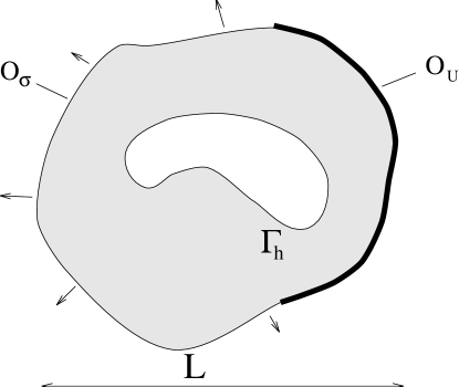
FIG. 1.: To calculate the energy release in the thermodynamic limit we specify displacements along $O_{U}$ and stresses along $O_{\sigma}$.

We define the energy release due to the formation of a void in an infinite material as the energy in a previously stretched material, released by cutting out a hole in it and letting the hole boundary relax the stress: the deformation energy of the discarded piece is excluded. Let’s consider an infinite linear elastic material subject to stress fields $\sigma_{xx}^{\infty}$, $\sigma_{yy}^{\infty}$ and $\sigma_{xy}^{\infty}$ at infinity. We want to calculate the energy release $E_{\rm release}$ due to cutting out a hole with boundary $\Gamma_{h}$. We assume that the hole boundary is stress free and non self-intersecting as a result of the stress relaxation. $\Gamma_{b}$ denotes a regularization boundary with a characteristic size $L$. Before the void formation, displacements along $\Gamma_{b}$ are $\vec{U}_{1}^{b}=(u_{1}^{b},v_{1}^{b})$, while those along the prospective void contour $\Gamma_{h}$ correspondingly $\vec{U}_{1}^{h}=(u_{1}^{h},v_{1}^{h})$. Let $O_{\sigma}$ and $O_{U}$ be nonintersecting parts of $\Gamma_{b}$, such that $O_{\sigma}\cup O_{U}=\Gamma_{b}$. Along $O_{\sigma}$ we fix the stresses $\sigma_{xx}^{\infty}$, $\sigma_{yy}^{\infty}$ and $\sigma_{xy}^{\infty}$ as a function of position; along $O_{U}$ we fix the displacements to be $\vec{U}_{1}^{b}$ (Figure 1). In analogy to the usage in field theory, each choice of boundary conditions $O_{\sigma}$, $\sigma^{\infty}$, $O_{U}$, $U^{b}_{1}$ we call a regularization. For a fixed $L$ we calculate the energy release $E_{\rm release}^{L}$. The thermodynamic limit of the energy release is then given by

$$E_{\rm release}=\lim_{L\to\infty}E_{\rm release}^{L}.$$ (1)

Physically the described regularization means that we compute first the energy release due to the formation of the void $\Gamma_{h}$ in a finite size material with the boundary $\Gamma_{b}$, and then push the outer (regularization) boundary to infinity. We will show that defined as above, $E_{\rm release}$ is independent of a particular choice of $O_{\sigma}$ and $O_{U}$, even if they are themselves functions of $L$. The boundary condition with $O_{\sigma}=\Gamma_{b}$ is known as a “fixed tension boundary condition”, while that with $O_{U}=\Gamma_{b}$ is referred to as a “fixed grip boundary condition”.

Let’s first consider a straight cut. As shown by explicit calculation[10], the “fixed tension” and the “fixed grip” boundary conditions for the special case of a straight cut of length $\ell$ opened by a uniform isotropic tension $T$, give the same energy release

$$E_{\rm release}={{\pi T^{2}{\ell}^{2}(\chi+1)}\over{32\mu}}={{\pi T^{2}{\ell}^{2}}\over{4Y}}.$$ (2)

The material elastic constants $\mu$ and $\chi$ can be expressed through its Young’s modulus $Y$ and Poisson ratio $\sigma$ as follows

$$\mu = {Y\over{2(1+\sigma)}}$$ (3)

$$\chi = {{3-\sigma}\over{1+\sigma}}.$$ (4)

(The given value for $\chi$ corresponds to a plain stress in a three dimensional elastic theory; for a plain strain one should use $\chi=3-4\sigma$.) Note that (2) coincides with Griffith’s result. This result is not trivial! If one calculates the energy change in a region $\Gamma_{b}$ embedded in an infinite medium (i.e., neither fixing the displacements nor allowing them to relax at fixed stress), the energy release does depend on the shape of the boundary. The relaxations at the boundary scale like $1/L$: even as $L\to\infty$, integrated over the perimeter they must be included for a sensible thermodynamic limit.

For a general void, the energy release is a sum of the work performed by the external $(W_{e})$ and the internal $(W_{i})$ forces as a result of the void formation

$$E_{\rm release}^{L}=W_{e}+W_{i}.$$ (5)

Let $e_{ij}^{(1)}$, $\sigma_{ij}^{(1)}$ be the strain and stress fields of the first state before the cut is made and $e_{ij}^{(2)}$, $\sigma_{ij}^{(2)}$ define the fields of the second state with the void; finally displacements along $O_{\sigma}$ for the second state are $\vec{U}_{2}^{b}=(u_{2}^{b},v_{2}^{b})$ and displacements along the void boundary $\Gamma_{h}$ are given by $\vec{U}_{2}^{h}=(u_{2}^{h},v_{2}^{h})$. As the void boundary relaxes, the external forces do work

$$W_{e}=\int_{O_{\sigma}}\vec{F}_{n}(\vec{U}_{2}^{b}-\vec{U}_{1}^{b})d{\ell}_{1}$$ (6)

where $\vec{F}_{n}=(F_{n_{x}},F_{n_{y}})$ is the traction along $O_{\sigma}$ defined through the asymptotic stress fields

$$F_{n_{x}}=\sigma_{xx}^{\infty}n_{x}+\sigma_{xy}^{\infty}n_{y}$$ (7)

$$F_{n_{y}}=\sigma_{xy}^{\infty}n_{x}+\sigma_{yy}^{\infty}n_{y}$$ (8)

with $(n_{x},n_{y})$ being the outwards normal to $O_{\sigma}$. The work done by the internal forces is the change in the energy of the elastic deformation of the first and the second states

$$W_{i}={1\over 2}{\int\int}_{A}\sigma_{ij}^{(1)}e_{ij}^{(1)}dA-{1\over 2}{\int\int}_{A}\sigma_{ij}^{(2)}e_{ij}^{(2)}dA.$$ (9)

The integration in (9) is performed over the area $A$ of the material excluding the void; the summation over repeating indexes is assumed. As a consequence of Hook’s law,

$${\int\int}_{A}\sigma_{ij}^{(1)}e_{ij}^{(2)}dA={\int\int}_{A}\sigma_{ij}^{(2)}e_{ij}^{(1)}dA$$ (10)

so we can rewrite (9) as

$$W_{i}={1\over 2}{\int\int}_{A}(\sigma_{ij}^{(1)}+\sigma_{ij}^{(2)})(e_{ij}^{(1)}-e_{ij}^{(2)})dA.$$ (11)

Let’s introduce a plus state specified by the stresses $\sigma^{+}_{ij}=\sigma_{ij}^{(1)}+\sigma_{ij}^{(2)}$ and a minus state defined by the strain fields $e^{-}_{ij}=e_{ij}^{(1)}-e_{ij}^{(2)}$. Then the work of the internal forces $(\ref{9})$ is a mixed energy of the plus and the minus states. According to Betti’s theorem [16], the mixed energy equals one half the work done by the stresses of one state over the displacements of the other, no matter from what state the stresses or displacements are taken. With the stresses from the plus state and the displacements from the minus state we obtain

$$W_{i} = {1\over 2}\int_{O_{\sigma}}\vec{F}^{+}_{n}\vec{U}^{-}_{b}d{\ell}_{1}+{1\over 2}\oint_{\Gamma_{h}}\vec{F}^{+}_{h}\vec{U}^{-}_{h}d{\ell}_{h}$$ (12)

$$= {1\over 2}\int_{O_{\sigma}}(\vec{F}_{n}+\vec{F}_{n})(\vec{U}_{1}^{b}-\vec{U}_{2}^{b})d{\ell}_{1}$$ (14)

$$+{1\over 2}\oint_{\Gamma_{h}}(\vec{F}_{h}+\vec{0})(\vec{U}_{1}^{h}-\vec{U}_{2}^{h})d{\ell}_{h}$$

$$= \int_{O_{\sigma}}\vec{F}_{n}(\vec{U}_{1}^{b}-\vec{U}_{2}^{b})d{\ell}_{1}+{1\over 2}\oint_{\Gamma_{h}}\vec{F}_{h}(\vec{U}_{1}^{h}-\vec{U}_{2}^{h})d{\ell}_{h}$$ (15)

where a traction of the first state $\vec{F}_{h}$ is defined as in (7) through the stresses of the first state along $\Gamma_{h}$. From (5), (6) and (12) we find the regularized energy release[8],[9]

$$E_{\rm release}^{L}={1\over 2}\oint_{\Gamma_{h}}\vec{F}_{h}(\vec{U}_{1}^{h}-\vec{U}_{2}^{h})d{\ell}_{h}.$$ (16)

The thermodynamic limit (1) is then taken by simply replacing $\vec{U}_{2}^{h}$ with its value

$$\vec{U}_{\infty}^{h}=\lim_{L\to\infty}\vec{U}_{2}^{h}$$ (17)

for the infinite media. One can check (using for example the complex variable method described below) that the difference between two can at most be of order $O(1/L)$, thus according to (16) and (1) not contributing to $E_{\rm release}$. So we conclude that

$$E_{\rm release}={1\over 2}\oint_{\Gamma_{h}}\vec{F}_{h}(\vec{U}_{1}^{h}-\vec{U}_{\infty}^{h})d{\ell}_{h}.$$ (18)

Thus the total energy release is half the work done at the cut boundary. The above result is explicitly independent of a particular regularization from the discussed class as well as of the shape of the regularization contour $\Gamma_{b}$. It has a straightforward extension for a finite number of voids in a media. For a media with $n$ holes with contours $\{\Gamma_{h_{i}}\}$, (18) generalizes to

$$E_{\rm release}={1\over 2}\sum_{i=1}^{n}\oint_{\Gamma_{h_{i}}}\vec{F}_{h_{i}}(\vec{U}_{1}^{h_{i}}-\vec{U}_{\infty}^{h_{i}})d{\ell}_{h_{i}}.$$ (19)

The same class of regularizations gives well defined thermodynamic limit in a three dimensional case as well. The arguments are practically the same resulting in the energy release (18) with the only change in the use of surface integrals rather than the contour ones for the regularization and void boundaries.

In order to use (18) one has to know displacements along the void contour for the second state. For all but several simple cases this is a very complicated problem to approach analytically: at best, one can hope to get an asymptotic behavior of the displacement and stress fields. So for practical purposes we have to find an asymptotic analog of the above expression that would allow the calculation of the energy release from the asymptotic behavior of the displacement fields. To do this, it is convenient to specify the stresses at infinity — the regularization with $O_{U}=\emptyset$ and $O_{\sigma}=\Gamma_{b}$. As we have already shown, this does not restrict the applicability of the result. To get the asymptotic expression for the energy release we first note that elastic states one and two are each in equilibrium, so from Clapeyron’s theorem[16]

$${1\over 2}{\int\int}_{A}\sigma_{ij}^{(1)}e_{ij}^{(1)}dA = {1\over 2}\oint_{\Gamma_{b}}\vec{F}_{n}\vec{U}_{1}^{b}d{\ell}_{b}+{1\over 2}\oint_{\Gamma_{h}}\vec{F}_{h}\vec{U}_{1}^{h}d{\ell}_{h}$$ (20)

$${1\over 2}{\int\int}_{A}\sigma_{ij}^{(2)}e_{ij}^{(2)}dA = {1\over 2}\oint_{\Gamma_{b}}\vec{F}_{n}\vec{U}_{2}^{b}d{\ell}_{b}.$$ (21)

Which, following (5), (6) and (9) gives

$$E_{\rm release}^{L} = {1\over 2}\oint_{\Gamma_{b}}\vec{F}_{n}\vec{U}_{2}^{b}d{\ell}_{b}-{1\over 2}\oint_{\Gamma_{b}}\vec{F}_{n}\vec{U}_{1}^{b}d{\ell}_{b}$$ (23)

$$+{1\over 2}\oint_{\Gamma_{h}}\vec{F}_{h}\vec{U}_{1}^{h}d{\ell}_{h}.$$

Next, we break $\vec{U}_{2}^{b}$ into two pieces: displacements of the second elastic state for the infinite media along $\Gamma_{b}$, $\vec{U}_{f}^{b}$, and the boundary relaxation displacements, $\vec{U}_{r}^{b}$,

$$\vec{U}_{2}^{b}=\vec{U}_{f}^{b}+\vec{U}_{r}^{b}.$$ (24)

The boundary relaxation displacements comes from relaxing the the stresses along $\Gamma_{b}$ for the infinite material to comply with the thermodynamic limit prescription: the “fixed tension boundary condition”. For the energy release calculation it is sufficient to relax the stresses to $O(1/L^{3})$ — the stresses of order $O(1/L^{3})$ generate the relaxation displacements along $\Gamma_{b}$ of order $O(1/L^{2})$ and thus do not contribute to the energy release in the limit $L\to\infty$. So, from (1), (23) and (24)

$$E_{\rm release}=\lim_{L\to\infty}\biggl{\{} {1\over 2}\oint_{\Gamma_{b}}\vec{F}_{n}(\vec{U}_{f}^{b}+\vec{U}_{r}^{b})d{\ell}_{b}-{1\over 2}\oint_{\Gamma_{b}}\vec{F}_{n}\vec{U}_{1}^{b}d{\ell}_{b}$$ (26)

$$+{1\over 2}\oint_{\Gamma_{h}}\vec{F}_{h}\vec{U}_{1}^{h}d{\ell}_{h}\biggr{\}}.$$

This is the desired expression. One can see that (26) is nothing but the difference between the regularized elastic deformation energy of the infinite media with the void (the first integral) and the elastic energy stored in the same media before the formation of void, not accounting for the elastic energy of the void itself (the remaining two integrals). Although the asymptotic expression for the energy release may look more complicated than (18) and actually requires solving of two elastic problems, its use is justified because it is difficult to find displacements of the second state along the void contour.

III Energy release of “slightly” curvy cuts

Armed with the knowledge that the energy release is independent of the shape of the regularization boundary, we now turn to the calculation of the energy release due to the opening of a “slightly” curvy cut $\Gamma_{h}$ in a two dimensional isotropic linear elastic infinite media subject to a uniform isotropic tension $T$ at infinity. We find an amazingly simple answer: the energy release of a curvy cut coincides to cubic order with the energy release of the straight cut with the same end points.

An elastic state is completely defined once displacements $(u,v)$ are known everywhere. Rather than considering these two functions, Muskhelishvili[17] introduces two complex functions $\phi(z)$ and $\psi(z)$ that in equilibrium should be the functions of only one complex variable $z$ (i.e. do not depend $\overline{z}$). Moreover in our case (a uniform isotropic tension at infinity) $\phi(z)$ decomposes as

$$\phi(z) = {1\over 2}Tz+\phi_{0}(z)$$ (27)

The functions $\phi_{0}(z)$ and $\psi(z)$ are holomorphic in the complex $z$ plane including infinity but excluding the cut contour. This description associates the components of stress $(\sigma_{xx},\sigma_{yy},\sigma_{xy})$ and displacement $(u,v)$ to $(\phi,\psi)$ by the following relations

$$\sigma_{xx}+\sigma_{yy} = 2(\phi^{\prime}(z)+\overline{\phi^{\prime}(z)})$$ (28)

$$\sigma_{yy}-\sigma_{xx}+2i\sigma_{xy} = 2(\overline{z}\phi^{\prime\prime}(z)+\psi^{\prime}(x))$$ (29)

$$2\mu(u+iv) = \chi\phi(z)-z\overline{\phi^{\prime}(z)}-\overline{\psi(z)}$$ (30)

(The detailed discussion of the change of “variables” $(u,v)\to(\phi,\psi)$ along with the derivation of (27)-(28) can be found in [17].) Using a circular regularization contour ($\Gamma_{b}$ is a circle of radius $L$) and an expression analogous to (26), Sih and Liebowitz[11] explicitly computed stresses along the outer boundary $\Gamma_{b}$ and found the energy release

$$E_{\rm release}=-{{\pi T}\over{4\mu}}(1+\chi)\rm{Re}[y_{1}]$$ (31)

with $y_{1}$ being the residue of $\psi(z)$ at infinity (the $1/z$ coefficient in the expansion about $z=\infty$). Of course, to determine $y_{1}$ we still need to solve the asymptotics of the elasticity problem.

To illustrate the correspondence between the energy release of a curvy cut and the straight one with the same end points, let’s consider a rare example where it is possible to find an exact analytical solution. Suppose a material with a “smile” cut - an arc of a circle ABC - of total arc length $\ell$ (Figure 2) is subject to a uniform isotropic stretching $T$ at infinity. Expanding the exact answer in[17] about $z=\infty$, we find

$$\psi_{\rm ABC}(z)=-{{T\ell^{2}}\over{8z}}{{8\sin^{2}\theta/2}\over{\theta^{2}(3-\cos\theta)}}+O\biggl{(}{{1}\over{z^{2}}}\biggr{)}$$ (32)

which according to (31) gives the energy release $E_{\rm ABC}$

$$E_{\rm ABC}={{\pi T^{2}\ell^{2}}\over{32\mu}}(1+\chi){{8\sin^{2}\theta/2}\over{\theta^{2}(3-\cos\theta)}}.$$ (33)

On the other hand, for a straight cut AC of length $(\ell/\theta)\sin\theta$, the holomorphic function $\psi_{\rm AC}(z)$ has asymptotic behavior [17]

$$\psi_{\rm AC}(z)=-{{T\ell^{2}}\over{8z}}{{\sin^{2}\theta}\over{\theta^{2}}}+O\biggl{(}{{1}\over{z^{2}}}\biggr{)}$$ (34)

resulting in the energy release $E_{\rm AC}$

$$E_{\rm AC}={{\pi T^{2}\ell^{2}}\over{32\mu}}(1+\chi){{\sin^{2}\theta}\over{\theta^{2}}}.$$ (35)

For small $\theta$ we find from (33) and (35) the advertised result: the energy release of ABC coincides with that of AC to cubic order in $\theta$, but not to quartic order!

$$E_{\rm ABC} = {{\pi T^{2}\ell^{2}}\over{32\mu}}(1+\chi)\biggl{(}1-{{\theta^{2}}\over 3}+{{77\theta^{4}}\over{720}}+O(\theta^{6})\biggr{)}$$ (36)

$$E_{\rm AC} = {{\pi T^{2}\ell^{2}}\over{32\mu}}(1+\chi)\biggl{(}1-{{\theta^{2}}\over 3}+{{2\theta^{4}}\over{45}}+O(\theta^{6})\biggr{)}.$$ (37)

FIG. 2.: The “smile”-like cut ABC and the straight cut AC result in the same energy release to cubic order in $\theta$.

We proceed now with the general proof. First, an arbitrary cut is approximated by a finite number of line segments, parameterized by the kink angles $\alpha_{i}$ — the angles between consecutive kinks. The exact shape of the cut is then restored as the length of each link goes to zero (as their number goes to infinity). The energy release is evaluated to cubic order in the kink angles, e.g for the $n$ - kink regularization, the energy release $E_{n}(\{\alpha_{i}\})$ for a curvy cut with a fixed separation $\ell_{p}$ between the endpoints is approximated as

$$E_{n}(\{\alpha_{i}\}) = E^{(0)}+\sum_{i=1}^{n}E_{i}^{(1)}\alpha_{i}+\sum_{i=1}^{n}\sum_{j=1}^{n}E^{(2)}_{ij}\alpha_{i}\alpha_{j}$$ (39)

$$+\sum_{i=1}^{n}\sum_{j=1}^{n}\sum_{m=1}^{n}E^{(3)}_{ijm}\alpha_{i}\alpha_{j}\alpha_{m}+O(\alpha_{i}^{4})$$

where $E^{0}$ is the energy release for a straight cut of length $\ell_{p}$ and the coefficients $E_{i}^{(1)}$, $E^{(2)}_{ij}$ and $E^{(3)}_{ijm}$ depend only on the positions of the kinks along the cut. We claim that all coefficients up to cubic order are zero, and thus the energy of a curvy cut and the straight one with the same endpoints can differ only at $O(\alpha_{i}^{4})$.

That $E_{i}^{(1)}$ and $E_{ijm}^{(3)}$ (in fact, all terms odd in the kink angles) are zero follows from a symmetry argument: cuts (having the same number of segments with the corresponding segments being of the same length) with kink angles $\{\alpha_{i}\}$ and $\{-\alpha_{i}\}$ respectively, are mirror images to each other with respect to the first link. The boundary condition for our problem (a uniform tension at infinity) is reflection invariant, so

$$E_{n}(\{\alpha_{i}\})=E_{n}(\{-\alpha_{i}\})$$ (40)

which requires that all energy release terms odd in the kink angles vanish. To calculate $E_{ij}^{(2)}$ for a given pair of indexes we can put all kink angles to zero except for $\alpha_{i}$ and $\alpha_{j}$, reducing the $n$-kink problem to a two-kink one. From now on we will consider only the two-kink problem to quadratic order in the kink angles.

FIG. 3.: The two-kink cut ABCD can be considered as a deformation of a straight cut AD.

We choose the coordinate system $XY$ in the complex $z$ plane in such a way that the ends of the two-kink cut are on the $X$ axis, symmetric with respect to the $Y$ axis (Figure 3). Assuming a uniform isotropic tension $T$ at infinity we rewrite (31), explicitly indicating the dependence of the energy release on the kink angles

$$E_{2}(\alpha_{1},\alpha_{2})=-{{\pi T}\over{4\mu}}(1+\chi)\rm{Re}[y_{1}(\alpha_{1},\alpha_{2})]$$ (41)

where $y_{1}(\alpha_{1},\alpha_{2})$ is $1/z$ coefficient in the expansion of the function $\psi(z)$ at infinity. As discussed earlier in the section, $\psi(z)$ is a holomorphic function in the complex $z$ plane including infinity (the extended complex plane) but excluding the two-kink cut. The other function $\phi(z)$ that is necessary for the specification of the equilibrium elastic state satisfies (27) with $\phi_{0}(z)$ holomorphic in the same region as $\psi(z)$. The analytical functions $\phi(z)$ and $\psi(z)$ must provide a stress free cut boundary, which following[17] can be expressed as

$$if(\phi,\psi)=\bigg{[}\phi(z)+z\overline{\phi^{\prime}(z)}+\overline{\psi(z)}\bigg{]}\Bigg{|}_{W}^{X}=0$$ (42)

where $f=F_{x}+iF_{y}$ is the complex analog of the force acting on the portion of the cut boundary between points $W$ and $X$.

It is important to note that any two pairs of functions $(\phi_{0}^{1}(z),\psi^{1}(z))$ and $(\phi_{0}^{2}(z),\psi^{2}(z))$ that are holomorphic in the extended $z$ plane excluding the same curvy cut, and which provide the stress free cut boundaries to $O(\alpha^{3})$ (42), can differ only by $O(\alpha^{3})$ everywhere:

$$\delta\phi(z) = \phi_{0}^{1}(z)-\phi_{0}^{2}(z)=O(\alpha^{3})$$ (43)

$$\delta\psi(z) = \psi^{1}(z)-\psi^{2}(z)=O(\alpha^{3}).$$ (44)

This follows explicitly from Cauchy’s theorem, but also follows from the elastic theory. Each pair $(\phi_{0}^{1}(z)+Tz/2,\psi^{1}(z))$ or $(\phi_{0}^{2}(z)+Tz/2,\psi^{2}(z))$ defines the equilibrium elastic state with stresses of order $O(\alpha^{3})$ along the cut boundary and uniform isotropic stretching $T$ at infinity. So, $(\delta\phi(z),\delta\psi(z))$ corresponds to the equilibrium state with the specified stresses of order $O(\alpha^{3})$ along the cut boundary and zero tension at infinity. Thus (43) follows because the response to this force within linear elastic theory must be linear. The above argument guarantees that once we find $\phi_{0}(z)$ and $\psi(z)$ that satisfy the discussed constraints to $O(\alpha^{3})$, we can use them to calculate the energy release of the curvy cut to quadratic order.

Let functions $\phi^{s}(z)$ and $\psi^{s}(z)$ define the equilibrium elastic state of a material with a straight cut AD subject to a uniform tension $T$ at infinity. $\phi_{0}^{s}(z)=\phi^{s}(z)-Tz/2$ and $\psi^{s}(z)$ should then be holomorphic in the extended complex $z$ plane excluding the straight cut and should provide stress free boundaries along AD. Muskhelishvili finds[17]

$${{d\phi^{s}(z)}\over{dz}} = {T\over 2}{z\over{\sqrt{z^{2}-{\ell_{p}}^{2}/4}}}$$ (45)

$${{d\psi^{s}(z)}\over{dz}} = {T\over 8}{{z{\ell_{p}}^{2}}\over{(z^{2}-{\ell_{p}}^{2}/4)\sqrt{z^{2}-{\ell_{p}}^{2}/4}}}.$$ (46)

(To obtain $\phi^{s}(z)$ and $\psi^{s}(z)$ we integrate (45); the arbitrariness in the integration constants reflect the ambiguity in the displacements up to a rigid motion of the material as a whole.) Note that $\phi_{0}^{s}(z)$ and $\psi^{s}(z)$ can be “made” holomorphic everywhere in the complex $z$ plane excluding the two-kink cut ABCD, and thus can serve as a good starting point for the construction of $\phi_{0}(z)$ and $\psi(z)$. The process of an analytical continuation is demonstrated by Figure 4. $\phi_{0}^{s}(z)$ (or equivalently $\psi^{s}(z)$) is holomorphic in the $z$ plane excluding the straight cut AD (4a). Removing the region ABCDA (4b), we make it holomorphic in the complex plane excluding ABCDA. Now we analytically continue $\phi_{0}^{s}(z)$ from the link AD (4c) into the removed region (the continuation is possible explicitly using (45)). The obtained function becomes holomorphic everywhere in the complex $z$ plane excluding the two-kink cut ABCD (4d), moreover the original function and the one obtained through the analytical continuation coincide outside ABCDA.

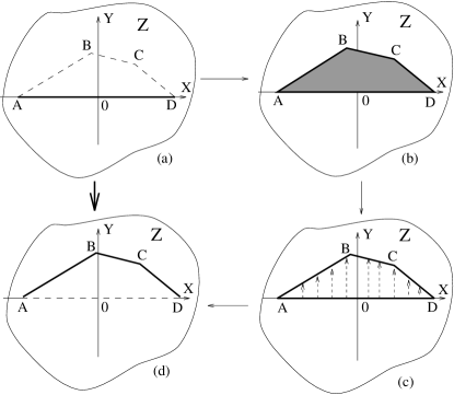
FIG. 4.: Functions $\phi_{0}^{s}(z)$ and $\psi^{s}(z)$ holomorphic in the complex $z$ plane excluding the straight cut AD (a), can be “made” holomorphic in the complex $z$ plane excluding the two-kink cut ABCD (d).

The idea of construction the holomorphic functions $\phi_{0}(z)$ and $\psi(z)$ is simple: we start with the functions $\phi_{0}^{s}(z)$ and $\psi^{s}(z)$ and calculate to quadratic order the stresses along the two-kink cut boundary ABCD under the analytical continuation as described by Figure 4. The stresses along the curvy cut boundary (Figure 5) are then compensated up to quadratic order in the kink angles by introducing counter-forces along the original (straight) cut, leading to corrected functions $\delta\phi^{c}(z)$ and $\delta\psi^{c}(z)$, where $\phi(z)=\phi^{s}(z)+\delta\phi^{c}(z)+O(\alpha^{3})$ and $\psi(z)=\psi^{s}(z)+\delta\psi^{c}(z)+O(\alpha^{3})$. For the calculation of the energy release (41) we need the real part of the residue of $\psi(z)$ at infinity: we will show that the residue of $\delta\psi^{c}(z)$ at infinity is zero and thus the residues of $\psi(z)$ and $\psi^{s}(z)$ at $z=\infty$ are the same — which means that the energy release for the curvy cut ABCD is the same as that of for the straight cut AD.

FIG. 5.: The stress free boundary of a two–kink ABCD cut (b) can be mimicked by applying the tangential force to the previously unstressed (a) straight cut boundary AD.

Let’s assume that points $W$ and $X$ are on the upper boundary of the link AB. From Figure 3, $z=t+i\beta(t+\ell_{p}/2)+O(\alpha^{3})$, where $t\in{\rm AB^{\prime}}$ and $\beta=(1-k_{1})\alpha_{1}+(1-k_{2})\alpha_{2}+O(\alpha^{3})$. Using (42) we find

$$i f(\phi_{0}^{s},\psi^{s})=\bigg{[}{\phi^{s}(t)}^{+}+t\overline{{{\phi^{s}(t)}^{\prime}}^{+}}+\overline{{\psi^{s}(t)}^{+}}\bigg{]}\Bigg{|}_{W}^{X}$$ (51)

$$+i\beta(t+\ell_{p}/2)\biggl{(}{{\phi^{s}(t)}^{\prime}}^{+}+\overline{{{\phi^{s}(t)}^{\prime}}^{+}}$$

$$\qquad-t\overline{{{\phi^{s}(t)}^{\prime\prime}}^{+}}-\overline{{{\psi^{s}(t)}^{\prime}}^{+}}\biggr{)}\bigg{|}_{W}^{X}$$

$$-{{\beta^{2}(t+\ell_{p}/2)^{2}}\over 2}\biggl{(}{{\phi^{s}(t)}^{\prime\prime}}^{+}+t\overline{{{\phi^{s}(t)}^{\prime\prime\prime}}^{+}}-2\overline{{{\phi^{s}(t)}^{\prime\prime}}^{+}}$$

$$\qquad+\overline{{{\psi^{s}(t)}^{\prime\prime}}^{+}}\biggr{)}\bigg{|}_{W}^{X}+O(\alpha^{3})$$

$$= 2\beta^{2}(t+\ell_{p}/2)^{2}{{\phi^{s}(t)}^{\prime\prime}}^{+}\bigg{|}_{W}^{X}+O(\alpha^{3}),$$ (52)

where $t$ runs along ${\rm AB^{\prime}}$; the $+$ superscript means that the values of $\phi_{0}^{s}(t)$ and $\psi(t)$ should be taken at the upper boundary of the straight cut. To obtain the second expression in (52) one can plug in the explicit form (45), or - more elegantly - note that for $t\in{\rm AB^{\prime}}$, $\phi^{s}(t)$ is pure imaginary and $\psi^{s}(z)^{\prime}=-z\phi^{s}(z)^{\prime\prime}$. Either way, it follows that the functions $\delta\phi^{c}(z)$ and $\delta\psi^{c}(z)$ satisfy

$$i\delta f = \bigg{[}{\delta\phi^{c}(t)}^{+}+t\overline{{{\delta\phi^{c}(t)}^{\prime}}^{+}}+\overline{{\delta\psi^{c}(t)}^{+}}\bigg{]}\Bigg{|}_{W}^{X}$$ (53)

$$= -2\beta^{2}(t+\ell_{p}/2)^{2}{{\phi^{s}(t)}^{\prime\prime}}^{+}\bigg{|}_{W}^{X}.$$ (54)

This is the force we need to add along the straight cut just below segment AB to cancel the stress along the curvy cut. Similar expressions can be found for the forces needed below BC and CD. To find $\delta\phi^{c}(z)$ and $\delta\psi^{c}(z)$ we have to solve the elasticity problem for the material with the straight cut AD, subject to these applied forces $i\delta f$ along the cut boundary. Fortunately, this problem allows a closed analytical solution[17]. Expanding the exact expression for $\delta\psi^{c}(z)$ in[17] we find

$$\delta\psi^{c}(z)={{\ell_{p}}\over{4\pi iz}}\oint_{\gamma}{\rm Re}\biggl{[}i\delta f(x(\sigma))\biggr{]}d\sigma+O\biggl{(}{1\over{z^{2}}}\biggr{)}$$ (55)

where the integration is along the unit circle $\gamma$ in the complex plane, and $i\delta f$ is a function of a variable point $x(\sigma)=\ell_{p}(\sigma+1/\sigma)/4$ along the straight cut boundary AD. Notice from (54) that $i\delta f$ is pure imaginary evaluated on the upper boundary of the link AB: in this case $|t|<\ell_{p}/2$, and so the argument of the square root in (45) is negative resulting in pure imaginary ${\phi^{s}(t)}^{\prime}$, thus ${\phi^{s}(t)}^{\prime\prime}$ is also pure imaginary. In fact, as it can be checked explicitly, ${\rm Re}\biggl{[}i\delta f\biggr{]}=0$ for arbitrary $W$ and $X$ along the cut boundary. So we conclude from (55) that the residue of $\delta\psi^{c}(z)$ at infinity is zero and thus the energy release for the curvy cut ABCD is the same as for the straight cut AD. The underling physical reason for this seeming remarkable coincidence is that to imitate the stress free curvy cut to quadratic order in the kink angles we have to apply only tangential force along the straight cut (pure imaginary $i\delta f$ means $F_{y}=0$), which do no work because a straight cut under a uniform isotropic tension at infinity opens up but does not shrink[17].

We find that the energy release $E(\ell_{p})$ of the curvy cut with projected distance $\ell_{p}$ between the endpoints is the same to quadratic order in the kink angles as the energy release of the straight cut of length $\ell_{p}$. The latter one is given by the second formula in (36) with $\theta=0$ (it also coincides with Griffith’s result (2))

$$E(\ell_{p})={{\pi T^{2}\ell_{p}^{2}}\over{32\mu}}(1+\chi).$$ (56)

The natural variables to describe the curvy cut are its total length $\ell$ and its curvature $k(x),\ x\in[0,\ell]$. In what follows we express (56) in these variables and find the normal modes of the curvature that diagonalize the energy release.

For the two-kink cut ABCD (Figure 3) of total length $\ell$ one can find

$$\ell_{p} = \ell\biggl{(}1-{{x_{1}(\ell-x_{1})}\over{2\ell^{2}}}\alpha_{1}^{2}-{{x_{1}(\ell-x_{2})}\over{\ell^{2}}}\alpha_{1}\alpha_{2}$$ (58)

$$-{{x_{2}(\ell-x_{2})}\over{2\ell^{2}}}\alpha_{2}^{2}\biggr{)}+O(\alpha^{3})$$

where $x_{1}$ and $x_{2}$ parameterize the kink positions: the length of the link AB is assumed to be $x_{1}$ and the length of the segment ABC equals $x_{2}$. Similarly, for the n-kink cut of total length $\ell$ with the kink angles $\{\alpha_{i}\}$ parameterized by their distance $\{x_{i}\}$ from the cut end

$$\ell_{p} = \ell\biggl{(}1-{1\over 2}\sum_{i,j=1}^{n}\alpha_{i}\alpha_{j}\biggl{[}-{{x_{i}x_{j}}\over{\ell^{2}}}+{{{\rm min}(x_{i},x_{j})}\over\ell}\biggr{]}\biggr{)}$$ (60)

$$+O(\alpha^{3}).$$

Expressing the kink angles through the local curvature of the curve, $\alpha_{i}=k(x_{i})\Delta x_{i}/\lambda$, we find the continuous limit of (60)

$$\ell_{p} = \ell\biggl{(}1-{1\over 2}\int_{0}^{\ell}\int_{0}^{\ell}{{dxdy}\over{\lambda^{2}}}k(x)M(x,y)k(y)\biggr{)}$$ (62)

$$+O({k(x)}^{3}),$$

with

$$M(x,y)=-{{xy}\over{\ell^{2}}}+{{{\rm min}(x,y)}\over\ell}$$ (63)

and the scale $\lambda$ is introduced to make the curvature dimensionless ($\lambda$ can be associated with the ultraviolet cutoff of the theory — roughly the interatomic distance). Substituting (63) into (56) we find the energy release $E(\ell,k(x))=E(\ell_{p})$ of the curvy cut in its intrinsic variables

$$E(\ell k(x))=$$ , (66)

$${{\pi T^{2}\ell^{2}}\over{32\mu}}(1+\chi)\biggl{(}1-\int_{0}^{\ell}\int_{0}^{\ell}{{dxdy}\over{\lambda^{2}}}k(x)M(x,y)k(y)\biggr{)}$$

$$+O({k(x)}^{3}).$$

To find the normal modes of the curvature we have to find the eigenvalues and eigenvectors of the operator $M(x,y)$. If $k_{n}(x)$ is an eigenvector of $M(x,y)$ with eigenvalue $\lambda_{n}$, then

$$\lambda_{n}k_{n}(x)=\int_{0}^{\ell}{{dy}\over\lambda}M(x,y)k_{n}(y).$$ (67)

From (63), $M(0,y)=0$ and $M(\ell,y)=0$ for arbitrary $y\in[0,\ell]$, so from (67) the eigenvectors of $M(x,y)$ must be zero at $x=0$ and $x=\ell$: $k_{n}(0)=k_{n}(\ell)=0$. An arbitrary function $k_{n}(x)$ with this property is given by the Fourier series

$$k_{n}(x)=\sum_{m=1}^{\infty}c_{m}\sqrt{{{2\lambda}\over{\ell}}}\sin{{\pi mx}\over{\ell}}$$ (68)

where the overall constant $\sqrt{2\lambda/\ell}$ is introduced to normalize the Fourier modes with the integration measure $dx/\lambda$ over $x\in[0,\ell]$. One can explicitly check from (67) that each Fourier mode $\sqrt{2\lambda/\ell}\sin(\pi mx/\ell)$ is in fact an eigenvector of $M(x,y)$ with the eigenvalue $\lambda_{m}=\ell/(\pi^{2}m^{2}\lambda)$. In terms of the amplitudes of the normal modes $\{c_{n}\}$, (66) is rewritten as

$$E(\ell,\{c_{n}\})={{\pi T^{2}\ell^{2}}\over{32\mu}}(1+\chi)\biggl{(}1-\sum_{n=1}^{\infty}{{\ell}\over{\pi^{2}n^{2}\lambda}}c_{n}^{2}\biggr{)}+O(c_{n}^{3}).$$ (69)

(69) is the main results of the section: we’ve calculated the energy release of an arbitrary curvy cut in its intrinsic variables — the total length $\ell$ and the curvature $k(x),\ x\in[0,\ell]$ — to quadratic order in $k(x)$ and found the normal modes of the curvature that diagonalize the energy release.

In conclusion we mention that the measure in the kink angle space is Cartesian — $\prod_{i}d\alpha_{i}$ — (and thus the functional measure $Dk(x)\equiv D\alpha(x)$ is Cartesian), so the measure in the vector space of the amplitudes of the normal modes $\{c_{n}\}$ is also Cartesian — $\prod_{n=1}^{\infty}dc_{n}$, because the Fourier transformation $\{k(x)\}\to\{c_{n}\}$ is orthonormal. This will be important in section V, where we will be integrating over crack shapes.

IV Surface phonons

In the previous sections we have extensively discussed the calculation of the energy release due to the equilibrium opening of a cut in an elastic material. Since our goal is to deal with cracks as thermal fluctuations, we must also deal with the more traditional elastic fluctuations — phonons, or sound. We find here that the bulk fluctuations decouple from the new surface phonon modes introduced by the cut. We discuss the quadratic fluctuations for linear elastic material with a straight cut of length $\ell$ subject to a uniform isotropic tension $T$ at infinity; more specifically, we calculate the energy release for the material with an arbitrary opening of the straight cut and we find collective coordinates (normal modes) that diagonalize the change in the energy.

An elastic state of the material can be defined through the specification of its displacements $\vec{U}=(u,v)$ at every point $(x,y)$. For the material with a cut, the fields $u(x,y)$ and $v(x,y)$ can in principle have a discontinuity along the cut: assuming that the cut is an interval $(x,y)=([-\ell/2,\ell/2],0)$,

$$2g_{x}(x)=u(x,0+)-u(x,0-),\mbox{\hskip 7.22743pt }{\rm for}\mbox{\hskip 7.22743pt }x\in[-\ell/2,\ell/2]$$ (70)

and

$$2g_{y}(x)=v(x,0+)-v(x,0-),\mbox{\hskip 7.22743pt }{\rm for}\mbox{\hskip 7.22743pt }x\in[-\ell/2,\ell/2]$$ (71)

may be nonzero. It is clear that the arbitrary state $\vec{U}$ can be decomposed into the superposition of two states $\vec{U}_{g}=(u_{g},v_{g})$ and $\vec{U}_{c}=(u_{c},v_{c})$, where $\vec{U_{g}}$ is the equilibrium state for given displacement discontinuity $(g_{x},g_{y})$ at the cut boundary (70-71) and tension $T$ at infinity that maximizes the energy release, and $\vec{U}_{c}$ given by $(u_{c},v_{c})=(u-u_{g},v-v_{g})$ is a continuous displacement field everywhere. Recall that the energy release is the sum of the work done by the external forces and the work done by the internal forces (5). We define the energy release $E$ for the elastic state $\vec{U}$ with respect to the equilibrium state of the material $\vec{U}_{0}=(u_{0},v_{0})$ without the cut under the same loading at infinity, as a limit of this difference for finite size samples with boundary $\Gamma_{b}$ and enclosed area $A$. We find following (5), (6) and (7)

$$E=\oint_{\Gamma_{b}}T\vec{n}(\vec{U}-\vec{U}_{0})d\ell+{1\over 2}\int\int_{A}(\sigma_{ij}^{0}e_{ij}^{0}-\sigma_{ij}e_{ij})dA$$ (72)

where $\sigma_{ij}^{0}$ and $e_{ij}^{0}$ are the stresses and strains of the equilibrium elastic state of the uncracked material $\vec{U}_{0}$; $\sigma_{ij}$ and $e_{ij}$ are the stresses and strains of the elastic state of material with the straight cut and displacement field $\vec{U}$; and $\vec{n}$ is a unit normal pointing outwards from the regularization boundary $\Gamma_{b}$. This argument is similar to that in the second section, but the elastic state $\vec{U}$ is not an equilibrium one and so the arguments there are not directly applicable. We rewrite the energy release (72) making use of the decomposition $\vec{U}=\vec{U}_{g}+\vec{U}_{c}$ to get

$$E = \oint_{\Gamma_{b}}T\vec{n}(\vec{U}_{g}-\vec{U}_{0})d\ell+{1\over 2}\int\int_{A}(\sigma_{ij}^{0}e_{ij}^{0}-\sigma_{ij}^{g}e_{ij}^{g})dA$$ (75)

$$-{1\over 2}\int\int_{A}\sigma_{ij}^{c}e_{ij}^{c}dA$$

$$+\oint_{\Gamma_{b}}T\vec{n}\vec{U}_{c}d\ell-{1\over 2}\int\int_{A}(\sigma_{ij}^{g}e_{ij}^{c}+\sigma_{ij}^{c}e_{ij}^{q})dA.$$

The first two integrals in (75) give the energy release for the equilibrium elastic state with the specified cut opening $(g_{x},g_{y})$ and tension $T$ at infinity. According to our decomposition this energy release is maximum for given $g_{x}(x)$ and $g_{y}(x)$ and thus can not increase linearly by tuning $\vec{U}_{c}$. The latter is true only if the last two integrals on the RHS of $(\ref{82})$ - linear in $\vec{U}_{c}$ - cancel each other. (This can be verified explicitly by integrating by parts the last integral on the RHS of (75) and using the fact that $\vec{U}_{g}$ is an equilibrium state.) Thus

$$E = \oint_{\Gamma_{b}}T\vec{n}(\vec{U}_{g}-\vec{U}_{0})d\ell+{1\over 2}\int\int_{A}(\sigma_{ij}^{0}e_{ij}^{0}-\sigma_{ij}^{g}e_{ij}^{g})dA$$ (77)

$$-{1\over 2}\int\int_{A}\sigma_{ij}^{c}e_{ij}^{c}dA:$$

the energy factors, and the last term representing the continuous degrees of freedom does not “feel” the presence of the cut and thus will have exactly the same spectrum as that of the uncracked material.

Although the elastic state $\vec{U}_{g}$ is an equilibrium one, the cut boundary is in general stressed, and so we still have to modify the result of the second section for the energy release (26). From the first equation in (21), the elastic energy of the uncracked material is given by

$${1\over 2}\int\int_{A}\sigma_{ij}^{0}e_{ij}^{0}dA={1\over 2}\oint_{\Gamma_{b}}T\vec{n}\vec{U}_{0}d\ell.$$ (78)

The elastic energy of the material with the cut (the second equation in (21)) is modified to incorporate the stressed cut boundary

$${1\over 2}\int\int_{A}\sigma_{ij}^{g}e_{ij}^{g}dA={1\over 2}\oint_{\Gamma_{b}}T\vec{n}\vec{U}_{g}d\ell+{1\over 2}\oint_{\Gamma_{h}}\vec{F}_{h}\vec{U}_{g}d\ell.$$ (79)

The second integral in (79) is over the cut boundary $\Gamma_{h}$ and $\vec{F_{h}}$ is the force we have to apply to the cut boundary to insure its displacements satisfy (70-71). With this change, following (77-79) we find that the energy release as given by (26) decreases by $\delta E$

$$\delta E={1\over 2}\oint_{\Gamma_{h}}\vec{F_{h}}\vec{U}_{g}d\ell.$$ (80)

In the spirit of the third section, the equilibrium elastic state $\vec{U}_{g}$ can be described by the analytical functions $\phi(z)$ and $\psi(z)$; $\phi_{0}(z)=\phi(z)-Tz/2$ and $\psi(z)$ are holomorphic in the extended complex $z$ plane excluding the straight cut and are constrained to provide displacement discontinuity $(g_{x},g_{y})$. The energy release $E_{g}$ is then smaller than the one given by (31) by $\delta E$

$$E_{g} = -{{\pi T}\over{4\mu}}(1+\chi){\rm Re}[y_{1}^{g}]-\delta E$$ (81)

where $y_{1}^{g}$ is the $1/z$ coefficient in the expansion of $\psi(z)$ at infinity.

To determine the functions $\phi_{0}(z)$ and $\psi(z)$ we conformally map the complex $z$ plane with the cut to the outside of the unit circle $\gamma$ (Figure 6)

$$z=\omega(\zeta)={{\ell}\over 4}\biggl{(}\zeta+{1\over{\zeta}}\biggr{)}$$ (82)

so that the unit circle in the $\zeta$ plane is mapped to the straight cut boundary $\Gamma_{h}$ in the original plane, $\Gamma_{h}=\omega(\gamma)$.

FIG. 6.: The determination of the holomorphic functions describing the equilibrium elastic state of the material with a straight cut is simplified in the conformal plane $\zeta$, where the unit circle $\gamma$ corresponds to cut boundary $\Gamma_{h}$ in the original $z$ plane.

The elasticity problem is reformulated in the conformal plane as follows: we have to find analytical functions $\phi_{g}(\zeta)=\phi(\omega(\zeta))$ and $\psi_{g}(\zeta)=\psi(\omega(\zeta))$, such that ${\phi_{g}}_{0}(\zeta)=\phi_{g}(\zeta)-\ell\zeta/4$ and $\psi_{g}(\zeta)$ are holomorphic in the extended complex $\zeta$ plane outside the unit circle and give the maximum energy release with displacement discontinuity $(g_{x},g_{y})$ at the cut boundary. We introduce

$$g(\sigma)=u_{g}+iv_{g}\bigg{|}_{\gamma}$$ (83)

where $\sigma=\exp(i\alpha)$, $\alpha\in[0,2\pi)$, is a parameterization of the unit circle $\gamma$. Since $\sigma$ and $1/\sigma$ represent opposite points across the cut, (70-71) require

$$g(\sigma)-g(1/\sigma)=2[g_{x}(\omega(\sigma))+ig_{y}(\omega(\sigma))],\ \alpha\in[0,\pi).$$ (84)

It is important to note that the equilibrium elastic state that maximizes the energy release for given displacement discontinuity $(g_{x},g_{y})$ is unique; on the other hand (84) determines only the asymmetric modes $g^{\rm asym}(\sigma)$ of the crack opening displacement for this state

$$2g^{\rm asym}(\sigma) = [u_{g}(\sigma)+iv_{g}(\sigma)]-[u_{g}(1/\sigma)+iv_{g}(1/\sigma)]$$ (85)

$$= 2[g_{x}(\omega(\sigma))+ig_{y}(\omega(\sigma))].$$ (86)

The symmetric modes $g^{\rm sym}(\sigma)$

$$2g^{\rm sym}(\sigma)=[u_{g}(\sigma)+iv_{g}(\sigma)]+[u_{g}(1/\sigma)+iv_{g}(1/\sigma)]$$ (87)

left unconstrained by (84), should then be relaxed to provide the maximum energy release for given $g^{\rm asym}(\sigma)$. Thus, to calculate the energy release $E_{g}$ of the elastic state $\vec{U}_{g}$ we first find the energy release $E(g)=E(g^{\rm asym}+g^{\rm sym})$ for the equilibrium state with an arbitrary displacement along the cut boundary $g(\sigma)$ and then maximize the result with respect to $g^{\rm sym}$

$$E_{g}=\max\limits_{g^{\rm sym}}E(g^{\rm asym}+g^{\rm sym}).$$ (88)

In what follows we will use $\phi_{\zeta}(\zeta)$ and $\psi_{\zeta}(\zeta)$ to describe the equilibrium elastic state with an arbitrary displacement $g(\sigma)$ along the cut boundary and tension $T$ at infinity. (The energy release for arbitrary $g(\sigma)$ is still given by (80-81).) Making the change of variables $z\to w(\zeta)$ in (28) and putting $\zeta=\sigma$ we obtain a constraint on $\phi_{\zeta}(\zeta)$ and $\psi_{\zeta}(\zeta)$ that guarantees the displacements along $\gamma$ to be $g(\sigma)$

$$\chi\phi_{\zeta}(\sigma)-{{\omega(\sigma)}\over{\overline{\omega^{\prime}(\sigma)}}}\overline{\phi_{\zeta}^{\prime}(\sigma)}-\overline{\psi_{\zeta}(\sigma)}=2\mu g(\sigma).$$ (89)

Once the solution $(\phi_{\zeta},\psi_{\zeta})$ of the elasticity problem is found, we can compute the correction (80) to the energy release. Introducing the polar coordinates $(\rho,\theta)$ (Figure 6) in the complex $\zeta$ plane, $\vec{F_{h}}=F_{\rho}\vec{\rho}+F_{\theta}\vec{\theta}$ and $\vec{U}_{g}=v_{\rho}\vec{\rho}+v_{\theta}\vec{\theta}$, and using $d\ell=|\omega^{\prime}(\sigma)||d\sigma|$ we find

$$\delta E = {1\over 2}\oint_{\gamma}\biggl{(}F_{\rho}v_{\rho}+F_{\theta}v_{\theta}\biggr{)}|\omega^{\prime}(\sigma)||d\sigma|$$ (90)

$$= {1\over 2}\oint_{\gamma}\biggl{(}\sigma_{\rho\rho}v_{\rho}+\sigma_{\rho\theta}v_{\theta}\biggr{)}|\omega^{\prime}(\sigma)||d\sigma|$$ (91)

where in the second equality we express the force through the stress tensor components: $F_{\rho}=\sigma_{\rho\rho}$ and $F_{\theta}=\sigma_{\rho\theta}$. The stress tensor components $\sigma_{\rho\rho}$ and $\sigma_{\rho\theta}$ are given in terms of the $\phi_{\zeta}(\zeta)$ and $\psi_{\zeta}(\zeta)$ functions that, as we already mentioned, completely determine the equilibrium elastic state. Muskhelishvili finds[17]

$$\sigma_{\rho\rho}-i\sigma_{\rho\theta} = {{\phi_{\zeta}^{\prime}(\zeta)}\over{\omega^{\prime}(\zeta)}}+{{\overline{\phi_{\zeta}^{\prime}(\zeta)}}\over{\overline{\omega^{\prime}(\zeta)}}}-{{\zeta^{2}}\over{\rho^{2}\overline{\omega^{\prime}(\zeta)}}}\biggl{\{}{{\overline{\omega(\zeta)}}\over{\omega^{\prime}(\zeta)}}\phi_{\zeta}^{\prime\prime}(\zeta)$$ (93)

$$-{{\overline{\omega(\zeta)}\omega^{\prime\prime}(\zeta)}\over{{\omega^{\prime}(\zeta)}}^{2}}\phi_{\zeta}^{\prime}(\zeta)+\psi_{\zeta}^{\prime}(\zeta)\biggr{\}}.$$

Noting that the transformation of the displacements along the unit circle in the Cartesian coordinates $(u_{g},v_{g})$, $g=u_{g}+iv_{g}$, to the polar coordinates $(v_{\rho},v_{\theta})$ is[17]

$$v_{\rho}+iv_{\theta}={1\over{\sigma}}{{\overline{\omega^{\prime}(\sigma)}}\over{|\omega^{\prime}(\sigma)|}}(u_{g}+iv_{g})={1\over{\sigma}}{{\overline{\omega^{\prime}(\sigma)}}\over{|\omega^{\prime}(\sigma)|}}g(\sigma),$$ (94)

we conclude from (90)

$$\delta E = {1\over 2}{\rm Re}\oint_{\gamma}(\sigma_{\rho\rho}-i\sigma_{\rho\theta})(v_{\rho}+iv_{\theta})|\omega^{\prime}(\sigma)||d\sigma|$$ (95)

$$= {1\over 2}{\rm Re}\oint_{\gamma}(\sigma_{\rho\rho}-i\sigma_{\rho\theta}){{\overline{\omega^{\prime}(\sigma)}}\over{\sigma}}g(\sigma){{d\sigma}\over{i\sigma}}$$ (96)

where $\sigma_{\rho\rho}-i\sigma_{\rho\theta}$ is given by (93) with $\zeta\to\sigma$ ($\rho\to 1$). From (81) and (95) we find the energy release $E(g)$

$$E(g) = -{{\pi T}\over{4\mu}}(1+\chi){\rm Re}[y_{1}(g)]$$ (98)

$$-{1\over 2}{\rm Re}\oint_{\gamma}(\sigma_{\rho\rho}-i\sigma_{\rho\theta}){{\overline{\omega^{\prime}(\sigma)}}\over{\sigma}}g(\sigma){{d\sigma}\over{i\sigma}}$$

where $y_{1}(g)$ is the $1/z$ coefficient in the expansion of $\psi_{\zeta}(\omega^{-1}(z))$ at $z=\infty$.

The equilibrium elastic problem for material with the straight cut allows a closed analytical solution for the arbitrary specified displacement $g(\sigma)$ along the unit circle in the conformal plane $\zeta$. Using the fact that ${\phi_{\zeta}}_{0}(\zeta)$ and $\psi_{\zeta}(\zeta)$ are holomorphic functions outside the unit circle that satisfy (89), Muskhelishvili finds[17]

$$\phi_{\zeta}(\zeta) = {{T\ell\zeta}\over 8}-{{2\mu}\over\chi}{1\over{2\pi i}}\oint_{\gamma}{{g(\sigma)d\sigma}\over{\sigma-\zeta}}+{{T\ell}\over{8\chi\zeta}}$$ (99)

$$\psi_{\zeta}(\zeta) = {{\mu}\over{\pi i}}\oint_{\gamma}{{\overline{g(\sigma)}d\sigma}\over{\sigma-\zeta}}+{{T\ell}\over 8}\biggl{(}{\chi\over\zeta}-{{2\zeta}\over{\zeta^{2}-1}}\biggr{)}$$ (101)

$$-\zeta{{1+\zeta^{2}}\over{\zeta^{2}-1}}\biggl{(}\phi_{\zeta}^{\prime}(\zeta)-{{T\ell}\over 8}\biggr{)}-{{\mu}\over{\pi i}}\oint_{\gamma}{{\overline{g(\sigma)}d\sigma}\over{\sigma}}.$$

Assuming that $g(\sigma)$ is smooth, we represent it by a convergent Fourier series

$$g(\sigma)=\sum_{-\infty}^{+\infty}(a_{n}+ib_{n})\sigma^{n}.$$ (102)

Using representation (102) for $g(\sigma)$ we find from (98) the energy release $E$

$$E(g) = {{\pi T\ell(1+\chi)}\over{4\chi}}(a_{-1}+\chi a_{1})$$ (105)

$$-2\pi\mu\sum_{n=1}^{+\infty}n\biggl{(}a_{n}^{2}+b_{n}^{2}+{{a_{-n}^{2}+b_{-n}^{2}}\over\chi}\biggr{)}$$

$$-{{\pi T^{2}{\ell}^{2}(1+\chi)}\over{128\mu}}\biggl{(}\chi-2+{1\over\chi}\biggr{)}.$$

(The computations are tedious, but straightforward: first we substitute (102) into (99) to find the solution of the elasticity problem in terms of the Fourier amplitudes $\{a_{n},b_{n}\}$, then we calculate the stress tensor components at the unit circle using (93), and finally plugging the result into (98) we obtain (105).) The next step is to relax the symmetric modes in the crack opening displacement given by $g(\sigma)$. From $(\ref{95})$ and $(\ref{86})$ we find

$$u_{g} = \sum_{n=1}^{+\infty}(a_{n}+a_{-n})\cos n\alpha+(b_{-n}-b_{n})\sin n\alpha$$ (106)

$$v_{g} = \sum_{n=1}^{+\infty}(b_{n}+b_{-n})\cos n\alpha+(a_{n}-a_{-n})\sin n\alpha$$ (107)

which with the change of variables

$$u_{n} = b_{-n}-b_{n}$$ (108)

$$v_{n} = a_{n}-a_{-n}$$ (109)

$$\tilde{u}_{n} = b_{n}+b_{-n}$$ (110)

$$\tilde{v}_{n} = a_{n}+a_{-n}$$ (111)

is rewritten as

$$u_{g} = \sum_{n=1}^{+\infty}\tilde{v}_{n}\cos n\alpha+u_{n}\sin n\alpha$$ (112)

$$v_{g} = \sum_{n=1}^{+\infty}\tilde{u}_{n}\cos n\alpha+v_{n}\sin n\alpha.$$ (113)

It is clear now that the asymmetric modes of the crack opening displacement are described by $\{u_{n},v_{n}\}$, while the symmetric ones are specified by $\{\tilde{u}_{n},\tilde{v}_{n}\}$. (Recall that points parameterized by $\sigma$ and $1/\sigma$ (or equivalently $\alpha$ and $-\alpha$) are opposite from one another across the cut.) The amplitudes $\{u_{n},v_{n}\}$ are uniquely determined for the given $(g_{x},g_{y})$. From (85) and (112)

$$g_{x}(\ell/2\cos\alpha)+ig_{y}(\ell/2\cos\alpha)=\sum_{n=1}^{+\infty}(u_{n}+iv_{n})\sin n\alpha$$ (114)

where $\alpha\in[0,\pi]$. Using the transformation inverse to (108) we can express the energy release (105) in terms of $\{u_{n},v_{n},\tilde{u}_{n},\tilde{v}_{n}\}$. The obtained expression is maximum for

$$\tilde{u}_{n} = u_{n}{{\chi-1}\over{1+\chi}}$$ (115)

$$\tilde{v}_{n} = v_{n}{{1-\chi}\over{1+\chi}},\mbox{\hskip 7.22743pt }n\neq 1$$ (116)

$$\tilde{v}_{1} = v_{1}{{1-\chi}\over{1+\chi}}+{{T\ell(\chi-1)}\over{8\mu}}$$ (117)

and gives the energy release $E_{g}$

$$E_{g}={{T\ell\pi}\over 2}v_{1}-{{2\pi\mu}\over{\chi+1}}\sum_{n=1}^{+\infty}n\biggl{(}u_{n}^{2}+v_{n}^{2}\biggr{)}.$$ (118)

Finally, the maximum of (118) is achieved for

$$u_{n}^{\rm max} = 0$$ (119)

$$v_{n}^{\rm max} = 0,\mbox{\hskip 7.22743pt }n\neq 1$$ (120)

$$v_{1}^{\rm max} = {{\pi T\ell(1+\chi)}\over{8\mu}}$$ (121)

and

$$E_{g}^{\rm max}={{\pi T^{2}\ell^{2}(1+\chi)}\over{32\mu}}$$ (122)

which, as one might expect, corresponds to the equilibrium opening of the cut[17] and the energy release associated with this opening (2). Expanding (118) about $\{u_{n}^{\rm max},v_{n}^{\rm max}\}$, $\{u_{n},v_{n}\}\to\{u_{n}^{\rm max}+u_{n},v_{n}^{\rm max}+v_{n}\}$, we find

$$E_{g}={{\pi T^{2}\ell^{2}(1+\chi)}\over{32\mu}}-{{2\pi\mu}\over{1+\chi}}\sum_{n=1}^{+\infty}n\biggl{(}u_{n}^{2}+v_{n}^{2}\biggr{)}.$$ (123)

Expression (123) is the desired result: we find that the crack opening displacements (specified on the unit circle in the conformal plane)

$$\{u,v\}=\bigg{\{} v_{n}{{1-\chi}\over{1+\chi}}\cos n\alpha+u_{n}\sin n\alpha,$$ (125)

$$u_{n}{{\chi-1}\over{1+\chi}}\cos n\alpha+v_{n}\sin n\alpha\bigg{\}}$$

imposed on the saddle point cut opening

$$\{u^{\rm max},v^{\rm max}\}=\{0,{{\pi T\ell(1+\chi)}\over{8\mu}}\sin\alpha\}$$ (126)

diagonalize the energy release and thus are the normal modes; with the excitation of the $n$-th normal mode with the amplitude $\{u_{n},v_{n}\}$ the energy release decreases by $2\pi\mu n(u_{n}^{2}+v_{n}^{2})/(1+\chi)$.

Although (118) has been derived for the material under uniform isotropic stretching at infinity, it can be reinterpreted to describe the minimum increase in the energy $\Delta E$ of the material under a uniform isotropic compression (pressure) $P$ at infinity, due to the opening of the straight cut with specified displacement discontinuity along its boundary. For the displacement discontinuity given by (114) we find similar to (118)

$$\Delta E={{P\ell\pi}\over 2}v_{1}+{{2\pi\mu}\over{\chi+1}}\sum_{n=1}^{+\infty}n\biggl{(}u_{n}^{2}+v_{n}^{2}\biggr{)}.$$ (127)

One can use the same arguments that lead to (77) to show that the crack opening normal modes (125) decouple from all continuous modes (that are present in the uncracked material) and thus leave their spectrum unchanged. The saddle point is however unphysical in this case: as follows from (126), ($T$ in (126) should be replaced with $-P$), it corresponds to a configuration where the material overlaps itself.

V The imaginary part of the partition function

Elastic materials at finite temperature undergo a phase transition to fracture at zero applied stress, similar to the first order phase transition in spin systems below the critical temperature at zero magnetic field. The free energy of an elastic material under a stretching load develops an imaginary part which determines the material lifetime with respect to fracture. The imaginary part of the free energy has an essential singularity at zero applied stress. In this section we calculate this singularity at low temperatures in a saddle point approximation including quadratic fluctuations.

Consider an infinite two-dimensional elastic material subject to a uniform isotropic stretching $T$ at infinity. Creation of a straight cut of length $\ell$ will increase the energy by $2\alpha\ell$, where $\alpha$ is the surface tension (the energy per unit length of edge), with a factor of $2$ because of the two free surfaces. On the other hand, the cut will open up because of elastic relaxation. Using (122) for the energy release we find the total energy $E(\ell)$ of the straight cut in equilibrium under stretching tension $T$:

$$E(\ell)=2\alpha\ell-{{\pi T^{2}\ell^{2}(1+\chi)}\over{32\mu}}.$$ (128)

Introducing

$$\ell_{c}={{32\mu\alpha}\over{\pi T^{2}(1+\chi)}}$$ (129)

we can rewrite the energy of the crack as

$$E(\ell)=2\alpha\ell-\alpha{\ell^{2}\over\ell_{c}}.$$ (130)

It follows that cracks with $\ell>\ell_{c}$ will grow, giving rise to the fracture of the material, while those with $\ell<\ell_{c}$ will heal — a result first obtained by Griffith[1]. At finite temperature a crack of any size can appear as a thermal fluctuation, which means that for arbitrary small stretching $T$ the true ground state of the system is fractured into pieces and so the free energy of the material cannot be analytical at $T=0$. Because the energy $E(\ell_{c})=\alpha\ell_{c}$ grows as $1/T^{2}$ as $T\rightarrow 0$, interactions between thermally nucleated cracks are unimportant at small $T$ and low temperatures (allowing us to use the “dilute gas approximation”).

The thermodynamic properties of a macroscopic system can be obtained from its partition function $Z$:

$$Z=\sum_{N=0}^{\infty}\sum_{n}\exp(-\beta E_{nN})$$ (131)

where the summation $N$ is over all possible numbers of particles (cracks in our case) and the summation $n$ is over all states of the system with $N$ cracks.

To begin with, let’s consider the partition function of the material with one cut $Z_{1}$

$$Z_{1}=\sum_{E}\exp(-\beta E)$$ (132)

where the summation is over all energy states of the material with a single cut. The calculation of the imaginary part of the partition function is dominated by a saddle point, that in our case is a straight cut of length $\ell_{c}$. The straight cut is the saddle point because it gains the most elastic relaxation energy for a given number of broken bonds (we explicitly show in section III that curving a cut reduces the energy release). For now we neglect all fluctuations of the critical droplet (the cut of length $\ell_{c}$) except for its uniform contraction or expansion — fluctuations in the length of the straight cut. Introducing the deviation $\Delta\ell$ in the cut length from the critical length $\ell_{c}$, $\Delta\ell=\ell-\ell_{c}$, we find from (130)

$$E=\alpha\ell_{c}-\alpha{{{\Delta\ell}^{2}}\over{\ell_{c}}}.$$ (133)

The fact that this degree of freedom has negative eigenvalue means that direct computation of the partition function yields a divergent result. A similar problem for the three-dimensional Ising model was solved by Langer[18]: one has to compute the partition function in a stable state $P=-T$ (compression), and then do an analytical continuation in parameter space to the state of interest. The free energy develops an imaginary part in the unstable state, related to the decay rate for fracture[19]: the situation is similar to that of barrier tunneling in quantum mechanics [20], where the imaginary part in the energy gives the decay rate of a resonance. We have explicitly implemented this prescription for the simplified calculation of the imaginary part of the free energy[13]: for the elastic material under a uniform isotropic compression at infinity allowing for the nucleation of straight cuts of an arbitrary length with an arbitrary elliptical opening (mode $v_{1}$ in (127)), we calculated the free energy in a dilute gas approximation. We carefully performed the analytical continuation to the metastable state describing the elastic material under the uniform isotropic stretching $T$ at infinity and found the imaginary part of the free energy

$${\rm Im}F^{\rm simple}(T)={2\over{\beta^{2}T\lambda^{2}}}\biggl{(}{\pi{{A}\over{\lambda^{2}}}}\biggr{)}\exp{\biggl{\{}{{-32\beta\mu\alpha^{2}}\over{\pi T^{2}(\chi+1)}}\biggr{\}}}$$ (134)

where $A$ is the area of the material and $\lambda$ is the ultraviolet cutoff of the theory. (The version of equation (134) as derived in[13], overcounts the contribution from zero-restoring-force modes $(2\pi A/\lambda^{2})$ by factor $2$. Because cracks tilted by $\theta$ and $\pi+\theta$ are identical, the proper contribution from rotations must be $\pi$, rather than $2\pi$.)

The alternative to this analytical continuation approach is to deform the integration contour over the amplitude of the unstable (negative eigenvalue) mode from the saddle point $\Delta\ell=0$ along the path of the steepest descent[18]. More precisely, we regularize the direct expression for the partition function

$$Z_{1}=Z_{0}\biggl{(}\pi{A\over{\lambda^{2}}}\biggr{)}\int_{-\ell_{c}}^{\infty}{{d\Delta\ell}\over\lambda}\exp\biggl{\{}-\beta\biggl{(}\alpha\ell_{c}-\alpha{{{\Delta\ell}^{2}}\over{\ell_{c}}}\biggr{)}\biggr{\}}$$ (135)

(which diverges at big $\Delta\ell$) by bending the $\Delta\ell$ integration contour from the saddle into the complex plane:

$$Z_{1} = Z_{0}\biggl{(}\pi{A\over{\lambda^{2}}}\biggr{)}\int_{-\ell_{c}}^{0}{{d\Delta\ell}\over\lambda}\exp\biggl{\{}-\beta\biggl{(}\alpha\ell_{c}-\alpha{{{\Delta\ell}^{2}}\over{\ell_{c}}}\biggr{)}\biggr{\}}$$ (137)

$$+Z_{0}\biggl{(}\pi{A\over{\lambda^{2}}}\biggr{)}\exp(-\beta\alpha\ell_{c})\int_{0}^{\pm i\infty}{{d\Delta\ell}\over\lambda}\exp\biggl{\{}\beta\alpha{{{\Delta\ell}^{2}}\over{\ell_{c}}}\biggl{\}}$$

In (135-137) the factor $(\pi A/{\lambda^{2}})$ comes from the zero-restoring-force modes for rotating and translating the cut, and $Z_{0}$ is the partition function for the uncracked material (unity for the present simplified calculation). The second integral in (137) generates the imaginary part of the partition function

$${\rm Im}Z_{1}=\pm{1\over 2}Z_{0}\biggl{(}\pi{A\over{\lambda^{2}}}\biggr{)}\exp(-\beta\alpha\ell_{c}){\biggl{(}{{\pi\ell_{c}}\over{\beta\alpha\lambda^{2}}}\biggr{)}}^{1/2}$$ (138)

with the $\pm$ sign corresponding to the analytical continuation to either side of the branch cut of the partition function. (We showed in[13] that partition function is an analytical function in complex $T$ with a branch cut along the line $T\in[0,+\infty$).) In a dilute gas approximation the partition function for the material with $N$ cuts $Z_{N}$ is given by

$$Z_{N}=Z_{0}{{{({Z_{1}}/Z_{0})}^{N}}\over{N!}}$$ (139)

which from (131) determines the material free energy

$$F=-{1\over\beta}\ln Z=-{1\over\beta}\ln\sum_{N=0}^{\infty}Z_{N}=-{1\over\beta}\ln Z_{0}-{1\over\beta}{{Z_{1}}\over{Z_{0}}}.$$ (140)

Following (138) and (140) we find the imaginary part of the free energy

$${\rm Im}F^{\rm simple}(T)=\pm {2\over{\beta^{2}T\lambda^{2}}}{\biggl{(}{{2\beta\mu\lambda^{2}}\over{\chi+1}}\biggr{)}}^{1/2}\biggl{(}{\pi{{A}\over{\lambda^{2}}}}\biggr{)}$$ (142)

$$\exp{\biggl{\{}{{-32\beta\mu\alpha^{2}}\over{\pi T^{2}(\chi+1)}}\biggr{\}}}$$

(142) differs from (134) only because for the calculation of the imaginary part of the free energy in[13] we used two degrees of freedom: the length of the cut and its elliptical opening, while in current calculation there is only one degree of freedom. One can immediately restore (134) by adding the $v_{1}$ mode of (123) to the energy of the elastic material (133) and integrating it out. From (123), the $v_{1}$ mode generates an additional multiplicative contribution $Z_{v_{1}}$ to the partition function for a single crack $Z_{1}$, and thus from (140) changes the imaginary part of the free energy for multiple cracks $F^{\rm simple}$, ${\rm Im}F^{\rm simple}\to Z_{v_{1}}{\rm Im}F^{\rm simple}$

$$Z_{v_{1}}=\int_{-\infty}^{+\infty}{{dv_{1}}\over{\lambda}}\exp\biggl{\{}-{{2\pi\mu\beta}\over{1+\chi}}v_{1}^{2}\biggr{\}}={\biggl{(}{{1+\chi}\over{2\mu\beta\lambda^{2}}}\biggr{)}}^{1/2}$$ (143)

which will cure the discrepancy between (142) and (134). Although the analytical continuation method is theoretically more appealing, the calculation of the imaginary part through the deformation of the integration contour of the unstable mode is more convenient once we include the quadratic fluctuations. It is clear that both methods (properly implemented) must give the same results.

We have already emphasized that the above calculation ignores the quadratic fluctuations about the saddle point (except for the uniform contraction or extension of the critical droplet), which may change the prefactor in the expression (142) for the imaginary part of the free energy and may renormalize the surface tension $\alpha$. There are three kinds of quadratic fluctuations we have to deal with. (I) Curvy cuts — changes in the shape of the tear in the material: deviations of the broken bonds from a straight-line configuration. (II) Surface phonons — thermal fluctuations of the free surface of the crack about its equilibrium opening. (III) Bulk phonons — thermal fluctuations of the elastic media that are continuous at the cut boundary. To incorporate these fluctuations we have to integrate out the quadratic deviation from the saddle point energy coming from their degrees of freedom (as we did for the surface phonon $v_{1}$ above). In all cases the answer will depend upon the microscopic lattice-scale structure of the material. In field-theory language, our theory needs regularization: we must decide exactly how to introduce the ultraviolet cut-off $\lambda$. Here we discuss the lattice regularization, where the cut-off is explicitly introduced by the interatomic distance, and $\zeta$-function regularization, common in field theory. We find that the precise form of the surface tension renormalization and the prefactor in the imaginary part of the free energy depends on the regularization prescription, but certain important quantities appear regularization independent.

The partition function of the elastic material with one cut $Z_{1}$ in the saddle point approximation (137), will develop a multiplicative factor $Z_{f}$ upon inclusion of the quadratic fluctuations $Z_{1}\to Z_{f}Z_{1}$ with

$$Z_{f}=\sum_{\Delta E}\exp(-\beta\Delta E).$$ (144)

A deviation $\Delta E$ from the saddle point energy is decomposed into three parts, with each part describing fluctuations of one of the mentioned three types

$$\Delta E = {{\alpha\l_{c}^{2}}\over{\pi^{2}\lambda}}\sum_{n=1}^{\infty}{1\over{n^{2}}}c_{n}^{2}+{{2\pi\mu}\over{1+\chi}}\sum_{n=1}^{\infty}n(u_{n}^{2}+v_{n}^{2})$$ (146)

$$+\Delta E_{\rm continuous}.$$

The first term in (146) accounts for the decrease in the energy release due to the curving of the saddle point cut of length $\ell_{c}$ with the curvature

$$k(x)=\sum_{n=1}^{\infty}c_{n}\sqrt{{{2\lambda}\over{\ell_{c}}}}\sin{{\pi nx}\over{\ell_{c}}},\ x\in[0,\ell_{c}].$$ (147)

(The first term in (146) follows from (69) with $l=l_{c}$ given by (129).) The second term in (146) describes the asymmetric modes in the thermal fluctuations of the free surface of the saddle point crack about its equilibrium opening shape

$$u^{\rm asym}(t)+iv^{\rm asym}(t)=\sum_{n=1}^{\infty}(u_{n}+iv_{n})\sin n\vartheta,\ \vartheta\in[-\pi,\pi)$$ (148)

where a point at the cut boundary is parameterized by its distance $t=\ell_{c}(1+\cos\vartheta)/2$ from the cut end; $\vartheta\in[-\pi,0)$ parameterize the lower boundary displacements and $\vartheta\in[0,\pi)$ parameterize the displacements of the upper boundary points. The symmetric modes of the crack opening about its equilibrium opening shape are assumed to relax providing the minimum increase in the elastic energy for a given $\{u_{n},v_{n}\}$. The latter guarantees that all additional modes with the continuous displacement at the cut boundary (the ones which give $\Delta E_{\rm continuous}$ — the last term in (146) describing the bulk phonons) decouple from $\{c_{n},u_{n},v_{n}\}$ and are the same as the ones for the uncracked material. (The arguments here are the same as those that were used in derivation of (77).) Since the curvature modes $\{c_{n}\}$ give the equilibrium energy of the curvy cut, the response of the surface phonons to such a curving is already incorporated, so the quadratic fluctuations $\{c_{n}\}$ can be calculated independently from the quadratic fluctuations $\{u_{n},v_{n}\}$. The latter means that there are no coupling between $\{c_{n}\}$ and $\{u_{n},v_{n}\}$ modes in (146), and the spectrum of $\{u_{n},v_{n}\}$ modes is the same as that for the straight cut of length $\ell_{c}$ (123).

The last thing we have to settle before the calculation of $Z_{f}$ is the proper integration measure for the surface phonon modes $\{u_{n},v_{n}\}$. (We argued in the conclusion of section III that the integration measure for the modes $c_{n}$ is Cartesian — $\prod_{n=1}^{\infty}dc_{n}$.) Here we show that because the functional measure in the displacement fields $(u(x,y),v(x,y))$ defined at each point of the material $(x,y)$ is naturally Cartesian — $D[u(x,y)/\lambda]D[v(x,y)/\lambda]$, the integration measure for the modes $\{u_{n},v_{n}\}$ must be of the form $\prod_{n=1}^{\infty}(1/2\pi)du_{n}dv_{n}/\lambda^{2}$.

An arbitrary elastic displacement field for the material with a curvy cut is defined by specifying its bulk part $(u_{\rm bulk}(x,y),v_{\rm bulk}(x,y))$ (point (x,y) can be anywhere except at the cut boundary) and the cut part $(u_{\rm cut}^{+}(t),u_{\rm cut}^{-}(t),v_{\rm cut}^{+}(t),v_{\rm cut}^{-}(t))$ (the cut displacements are defined along the cut and are parameterized by the distance $t=\ell_{c}(1+\cos\vartheta)/2,\ \vartheta\in[0,\pi)$ from the cut end; the $+$ and $-$ superscripts are correspondingly the displacements at the upper and the lower boundary of the cut). It is helpful to visualize the introduction of the cut into the material as splitting in half each of the atoms of the material along the cut boundary. Then, the bulk part of the displacement field combines degrees of freedom of all atoms left untouched by splitting and the cut part describes the displacements of the split ones. Note that the splitting increases the total number of the degrees of freedom. The original measure is naturally

$$D[u_{\rm bulk}(x,y)/\lambda] D[v_{\rm bulk}(x,y)/\lambda]D[u_{\rm cut}(t)^{+}u_{\rm cut}(t)^{-}/\lambda^{2}]$$ (150)

$$D[v_{\rm cut}(t)^{+}v_{\rm cut}(t)^{-}/\lambda^{2}]$$

First we separate the symmetric and asymmetric parts in the crack opening displacement

$$u^{\rm asym}(t) = {1\over 2}\biggl{(}u_{\rm cut}^{+}(t)-u_{\rm cut}^{-}(t)\biggr{)}$$ (151)

$$v^{\rm asym}(t) = {1\over 2}\biggl{(}v_{\rm cut}^{+}(t)-v_{\rm cut}^{-}(t)\biggr{)}$$ (152)

$$u^{\rm sym}(t) = {1\over 2}\biggl{(}u_{\rm cut}^{+}(t)+u_{\rm cut}^{-}(t)\biggr{)}$$ (153)

$$v^{\rm sym}(t) = {1\over 2}\biggl{(}v_{\rm cut}^{+}(t)+v_{\rm cut}^{-}(t)\biggr{)}$$ (154)

Because the Jacobian of the transformation

$$(u_{\rm cut}(t)^{+},u_{\rm cut}(t)^{-},v_{\rm cut}(t)^{+},v_{\rm cut}(t)^{-})\to$$ (155)

$$(u^{\rm asym}(t),v^{\rm asym}(t),u^{\rm sym}(t),v^{\rm sym}(t))$$ (156)

is constant

$$\Bigg{|}{{\partial(u_{\rm cut}(t)^{+},u_{\rm cut}(t)^{-},v_{\rm cut}(t)^{+},v_{\rm cut}(t)^{-})}\over{\partial(u^{\rm asym}(t),v^{\rm asym}(t),u^{\rm sym}(t),v^{\rm sym}(t))}}\Bigg{|}={1\over 4},$$ (157)

the integration measure remains Cartesian:

$$D[u_{\rm bulk}(x,y)/\lambda] D[v_{\rm bulk}(x,y)/\lambda]D[u^{\rm sym}(t)v^{\rm sym}(t)/\lambda^{2}]$$ (159)

$$D[u^{\rm asym}(t)v^{\rm asym}(t)/4\lambda^{2}].$$

Now we can combine the bulk and the symmetric cut part of the measure by introducing the continuous displacement fields $(u_{c}(x,y),v_{c}(x,y))$ everywhere, including the cut boundary.(In our atomic picture, the symmetric modes of the cut part of the displacement fields represent the displacements of the split atoms as if they were whole, and so it is natural to combine these degrees of freedom with the bulk ones. Obtained as a result of such combination the continuous degrees of freedom are indistinguishable from the degrees of freedom of the uncracked material.) The integration measure becomes

$$D[u_{c}(x,y)/\lambda]D[v_{c}(x,y)/\lambda]D[u^{\rm asym}(t)v^{\rm asym}(t)/4\lambda^{2}].$$

According to our decomposition, we specify the asymmetric cut opening and find the equilibrium displacement fields that minimize the increase in the elastic energy. In other words, given $(u^{\rm asym}(t),v^{\rm asym}(t))$ determine $(u_{c}^{\rm min}(u^{\rm asym},v^{\rm asym}),v_{c}^{\rm min}(u^{\rm asym},v^{\rm asym}))$. The transformation

$$u_{c}(x,y) = u_{c}^{\rm min}(u^{\rm asym},v^{\rm asym})+\tilde{u}_{c}(x,y)$$ (160)

$$v_{c}(x,y) = v_{c}^{\rm min}(u^{\rm asym},v^{\rm asym})+\tilde{v}_{c}(x,y)$$ (161)

then completely decouple the surface phonon modes and the continuous modes that contribute to $\Delta E_{\rm continuous}$ in (146). The Jacobian of the transformation

$$(u_{c}(x,y),v_{c}(x,y),u^{\rm asym}(t),v^{\rm asym}(t))\to$$ (162)

$$(\tilde{u}_{c}(x,y),\tilde{v}_{c}(x,y),u^{\rm asym}(t),v^{\rm asym}(t))$$ (163)

is unity (the transformation is just a functional shift) and so the measure remains unchanged

$$D[\tilde{u}_{c}(x,y)/\lambda]D[\tilde{v}_{c}(x,y)/\lambda]D[u^{\rm asym}(t)v^{\rm asym}(t)/4\lambda^{2}].$$

The Fourier transformation (148) is orthogonal, but the Fourier modes are not normalized:

$$\int_{0}^{\pi}d\vartheta\ \sin^{2}n\vartheta={\pi\over 2}.$$ (164)

The latter means that at the final stage of the change of variables $(u^{\rm asym}(t),v^{\rm asym}(t))\to\{u_{n},v_{n}\}$ there appear the Jacobian $\prod_{n=1}^{\infty}(2/\pi)$, and so we end up with the integration measure $\prod_{n=1}^{\infty}(1/2\pi)du_{n}dv_{n}/\lambda^{2}$.

From (144-146) with the proper integration measure over the surface phonon modes we find

$$Z_{f} = \prod_{n=1}^{\infty}\int_{-\infty}^{+\infty}dc_{n}\exp\biggl{\{}-\beta{{\alpha\l_{c}^{2}}\over{\pi^{2}\lambda n^{2}}}c_{n}^{2}\biggr{\}}$$ (167)

$$\prod_{n=1}^{\infty}{\int\int}_{-\infty}^{+\infty}{1\over{2\pi}}{{du_{n}dv_{n}}\over{\lambda^{2}}}\exp\biggl{\{}-\beta{{2\pi\mu n}\over{1+\chi}}(u_{n}^{2}+v_{n}^{2})\biggr{\}}$$

$$Z_{\rm continuous}$$

$$= \prod_{n=1}^{\infty}{\biggl{(}{{\pi^{3}\lambda n^{2}}\over{\beta\alpha\ell_{c}^{2}}}\biggr{)}}^{1/2}\ \prod_{n=1}^{\infty}{{1+\chi}\over{4\pi\beta\mu\lambda^{2}n}}\ Z_{\rm continuous}$$ (168)

where

$$Z_{\rm continuous}=\sum_{\Delta E_{\rm continuous}}\exp(-\beta\Delta E_{\rm continuous}).$$ (169)

Because $\Delta E_{\rm continuous}$ corresponds to the degrees of freedom of the uncracked material (with the same energy spectrum), $Z_{\rm continuous}$ contributes to the partition function $Z_{0}$ of the material without the crack, which according to (140) drops out from the calculation of the imaginary part of the free energy.

All the products over $n$ in these expressions diverge: we need a prescription for cutting off the modes at short wavelengths (an ultraviolet cutoff).

First we’ll consider the $\zeta$-function regularization. In this regularization prescription[21], the infinite product of the type $D=\prod_{n=1}^{\infty}\lambda_{n}$ is evaluated by introducing the function $D_{\zeta}(s)$

$$D_{\zeta}(s)=\sum_{n=1}^{\infty}{1\over{\lambda_{n}^{s}}}$$ (170)

so that

$$D=\exp(-D_{\zeta}^{\prime}(0)).$$ (171)

It is assumed that the sum (170) is convergent in some region of the complex $s$ plane and that it is possible to analytically continue $D_{\zeta}(s)$ from that region to $s=0$. From (168) we find

$$Z_{f}=D_{1}D_{2}Z_{\rm continuous}$$ (172)

where $D_{1}$ and $D_{2}$ are obtained following (171) from the corresponding $\zeta$-functions: ${D_{1}}_{\zeta}(s)$ and ${D_{2}}_{\zeta}(s)$

$${D_{1}}_{\zeta}(s) = {\biggl{(}{{\beta\alpha\ell_{c}^{2}}\over{\pi^{3}\lambda}}\biggr{)}}^{s/2}\sum_{n=1}^{\infty}{1\over{n^{s}}}={\biggl{(}{{\beta\alpha\ell_{c}^{2}}\over{\pi^{3}\lambda}}\biggr{)}}^{s/2}\zeta_{R}(s)$$ (173)

$${D_{2}}_{\zeta}(s) = {\biggl{(}{{4\pi\beta\mu\lambda^{2}}\over{1+\chi}}\biggr{)}}^{s}\sum_{n=1}^{\infty}n^{s}={\biggl{(}{{4\pi\beta\mu\lambda^{2}}\over{1+\chi}}\biggr{)}}^{s}\zeta_{R}(-s).$$ (174)

$\zeta_{R}(s)$ in (173) is the standard Riemann $\zeta$-function, holomorphic everywhere in the complex $s$ plane except at $s=1$. Noting that $\zeta(0)=-1/2$ and $\zeta^{\prime}(0)=-(\ln 2\pi)/2$ we find from (171-173)

$$Z_{f}={\biggl{(}{{4\beta\alpha\ell_{c}^{2}}\over{\pi\lambda}}\biggr{)}}^{1/4}{\biggl{(}{{2\beta\mu\lambda^{2}}\over{1+\chi}}\biggr{)}}^{1/2}Z_{\rm continuous}.$$ (175)

From (140) and (168) we find the imaginary part of the free energy in the $\zeta$-function regularization

$${\rm Im}F^{\zeta}={\biggl{(}{{16\beta^{3}\alpha\mu^{2}\lambda^{5}}\over{\pi{(1+\chi)}^{2}}}\biggr{)}}^{1/4}{\biggl{(}{{\ell_{c}}\over{\lambda}}\biggr{)}}^{1/2}{\rm Im}F^{\rm simple}$$ (176)

where ${\rm Im}F^{\rm simple}$ is given by (142).

Second, we consider lattice regularization — which is more elaborate. We represent a curvy cut by $N+1=\ell_{c}/\lambda$ segments of equal length parameterized by the kink angles $\{\alpha_{i}\},\ i\in[1,N]$. With our conventional parameterization of the cut $t=\ell_{c}(1+\cos\vartheta)/2,\ \vartheta[-\pi,\pi)$, the asymmetric modes of the crack opening displacements $\{u^{\rm asym}(t),v^{\rm asym}(t)\}$ are linear piecewise approximation for given asymmetric displacements of the “split” kink atoms $\{u^{\rm asym}_{i},v^{\rm asym}_{i}\},\ i\in[1,N]$. More precisely, if $t_{i}$ and $t_{i+1}$ parameterize the adjacent kinks, we assume

$$u^{\rm asym}(t) = u^{\rm asym}_{i}+{{u^{\rm asym}_{i+1}-u^{\rm asym}_{i}}\over{t_{i+1}-t_{i}}}(t-t_{i})$$ (177)

$$v^{\rm asym}(t) = v^{\rm asym}_{i}+{{v^{\rm asym}_{i+1}-v^{\rm asym}_{i}}\over{t_{i+1}-t_{i}}}(t-t_{i})$$ (178)

for $t\in[t_{i},t_{i+1}]$. From the integration measure arguments for the $\zeta$-function regularization, it is clear that the integration measure in this case must be $\prod_{i=1}^{N}d\alpha_{i}\prod_{i=1}^{N}du^{\rm asym}_{i}dv^{\rm asym}_{i}/4\lambda^{2}$. Now we have to write down the lattice regularization of the quadratic deviation $\Delta E$ from the saddle point energy (146). From (56) and (60), the curving of the critical cut $\ell_{c}$ will reduce the energy release by $\Delta E_{c}$

$$\Delta E_{c} = {{T^{2}\pi(1+\chi)\ell_{c}^{2}}\over{32\mu}}\sum_{i,j=1}^{N}\alpha_{i}\alpha_{j}M^{c}_{ij}$$ (179)

$$= \alpha\ell_{c}\sum_{i,j=1}^{N}\alpha_{i}\alpha_{j}M^{c}_{ij}$$ (180)

where

$$M^{c}_{ij}=-{{ij}\over{{(N+1)}^{2}}}+{{{\rm min}(i,j)}\over{N+1}}.$$ (181)

From (146) the surface phonon contribution to $\Delta E$ is given by

$$\Delta E_{p}={{2\pi\mu}\over{1+\chi}}\sum_{n=1}^{+\infty}n(u_{n}^{2}+v_{n}^{2})$$ (182)

where from (148)

$$u_{n} = {2\over\pi}\int_{0}^{\pi}d\vartheta\ u^{\rm asym}(t(\vartheta))\sin n\vartheta$$ (183)

$$v_{n} = {2\over\pi}\int_{0}^{\pi}d\vartheta\ v^{\rm asym}(t(\vartheta))\sin n\vartheta.$$ (184)

In principle, for a given piecewise approximation of the asymmetric modes (177) determined by $\{u^{\rm asym}_{i},v_{i}^{\rm asym}\}$, $i\in[1,N]$, one could calculate the Fourier amplitudes according to (183) and then plug the result into (182) to obtain $\Delta E_{p}$ in terms of $\{u^{\rm asym}_{i},v_{i}^{\rm asym}\}$. We will use another approach. Using $u^{\rm asym}(0)=u^{\rm asym}(\ell_{c})=0$ (with the same equalities for $v^{\rm asym}(t)$) we integrate (183) by parts to obtain

$$u_{n} = {2\over\pi}\int_{0}^{\pi}d\vartheta\ {{du^{\rm asym}(t(\vartheta))}\over{d\vartheta}}{{\cos n\vartheta}\over n}$$ (185)

$$v_{n} = {2\over\pi}\int_{0}^{\pi}d\vartheta\ {{dv^{\rm asym}(t(\vartheta))}\over{d\vartheta}}{{\cos n\vartheta}\over n}.$$ (186)

Substituting (185) into (182) we find

$$\Delta E_{p} = {{8\mu}\over{\pi(1+\chi)}}\int_{0}^{\pi}\int_{0}^{\pi}d\vartheta_{1}d\vartheta_{2}\biggl{[}{{du^{\rm asym}(\vartheta_{1})}\over{d\vartheta_{1}}}{{du^{\rm asym}(\vartheta_{2})}\over{d\vartheta_{2}}}$$ (188)

$$+{{dv^{\rm asym}(\vartheta_{1})}\over{d\vartheta_{1}}}{{dv^{\rm asym}(\vartheta_{2})}\over{d\vartheta_{2}}}\biggr{]}K(\vartheta_{1},\vartheta_{2})$$

where

$$K(\vartheta_{1},\vartheta_{2}) = \sum_{n=1}^{\infty}{{\cos n\vartheta_{1}\cos n\vartheta_{2}}\over n}.$$ (189)

Following[22]

$$\sum_{k=1}^{\infty}{{\cos kx}\over{k}}={1\over 2}\ln{1\over{2(1-\cos x)}},$$ (190)

we find an analytical expression for the kernel (189)

$$K(\vartheta_{1},\vartheta_{2})=-{1\over 2}\ln 2-{1\over 2}\ln|\cos\vartheta_{1}-\cos\vartheta_{2}|.$$ (191)

Finally, introducing $M_{ij}^{p}$ from

$$\sum_{i,j=1}^{N} \biggl{(}u^{\rm asym}_{i}u^{\rm asym}_{j}+v^{\rm asym}_{i}v^{\rm asym}_{j}\biggr{)}M_{ij}^{p}$$ (192)

$$= \int_{0}^{\pi}\int_{0}^{\pi}d\vartheta_{1}d\vartheta_{2}\biggl{[}{{du^{\rm asym}(\vartheta_{1})}\over{d\vartheta_{1}}}{{du^{\rm asym}(\vartheta_{2})}\over{d\vartheta_{2}}}$$ (194)

$$+{{dv^{\rm asym}(\vartheta_{1})}\over{d\vartheta_{1}}}{{dv^{\rm asym}(\vartheta_{2})}\over{d\vartheta_{2}}}\biggr{]}K(\vartheta_{1},\vartheta_{2})$$

we obtain

$$\Delta E_{p}={{8\mu}\over{\pi(1+\chi)}}\sum_{i,j=1}^{N}\biggl{(}u^{\rm asym}_{i}u^{\rm asym}_{j}+v^{\rm asym}_{i}v^{\rm asym}_{j}\biggr{)}M_{ij}^{p}.$$ (195)

To calculate $M_{ij}^{p}$ we substitute (177) directly into the RHS of (194) and read off the corresponding coefficient, given by the following three equations:

$$M_{ij}^{p}=f_{2}(i,j)+f_{2}(i+1,j+1)-f_{2}(i+1,j)$$ (196)

$$\qquad\quad-f_{2}(i,j+1)$$ (197)

(198)

$$f_{2}(i,j)={3\over 4}+{1\over{(\cos\vartheta_{i-1}-\cos\vartheta_{i})(\cos\vartheta_{j-1}-\cos\vartheta_{j})}}\biggl{[}$$ (199)

$$f_{1}(i,j)+f_{1}(i-1,j-1)-f_{1}(i-1,j)-f_{1}(i,j-1)\biggr{]}$$ (200)

(201)

$$f_{1}(i,j)=$$ (202)

$$\cases{{{{(\cos\vartheta_{i}-\cos\vartheta_{j})}^{2}}\over 4}\ln\bigg{|}\sin{{\vartheta_{i}-\vartheta_{j}}\over 2}\sin{{\vartheta_{i}+\vartheta_{j}}\over 2}\bigg{|},&if $i\neq j$;\cr 0,&otherwise,\cr}$$ (203)

(204)

where $\vartheta_{0}=0$, $\vartheta_{N+1}=\pi$, and $\vartheta_{i}$ parameterizes the $i$-th kink (kinks are equally spaced in real space):

$$\vartheta_{i}=\arccos\biggl{(}1-{{2i}\over{N+1}}\biggr{)},\ i\in[1,N].$$ (205)

From (180) and (195) we find the quadratic deviation from the saddle point energy

$$\Delta E = \Delta E_{c}+\Delta E_{p}+\Delta E_{\rm continuous}$$ (206)

$$= \alpha\ell_{c}\sum_{i,j=1}^{N}\alpha_{i}\alpha_{j}M^{c}_{ij}+{{8\mu}\over{\pi(1+\chi)}}\sum_{i,j=1}^{N}\biggl{(}u^{\rm asym}_{i}u^{\rm asym}_{j}$$ (208)

$$+v^{\rm asym}_{i}v^{\rm asym}_{j}\biggr{)}M_{ij}^{p}+\Delta E_{\rm continuous}.$$

Thus the multiplicative factor $Z_{f}$ to the partition function of the elastic material with one cut in the lattice regularization is given by

$$Z_{f} = \prod_{n=1}^{N}\int_{-\infty}^{+\infty}d\alpha_{n}\exp\biggl{\{}-\beta\alpha\ell_{c}\sum_{i,j=1}^{N}\alpha_{i}\alpha_{j}M^{c}_{ij}\biggr{\}}$$ (212)

$$\prod_{n=1}^{N}\int\int_{-\infty}^{+\infty}{{du_{n}^{\rm asym}dv_{n}^{\rm asym}}\over{4\lambda^{2}}}\exp\biggl{\{}-\beta{{8\mu}\over{\pi(1+\chi)}}$$

$$\sum_{i,j=1}^{N}\biggl{(}u^{\rm asym}_{i}u^{\rm asym}_{j}+v^{\rm asym}_{i}v^{\rm asym}_{j}\biggr{)}M_{ij}^{p}\biggr{\}}$$

$$Z_{\rm continuous}$$

$$= {\biggl{(}{{\pi}\over{\beta\alpha\ell_{c}}}\biggr{)}}^{N/2}{\det}^{-1/2}M_{ij}^{c}\ {\biggl{(}{{\pi^{2}(1+\chi)}\over{32\beta\mu\lambda^{2}}}\biggr{)}}^{N}$$ (214)

$${\det}^{-1}M_{ij}^{p}\ Z_{\rm continuous}$$

where $Z_{\rm continuous}$ is given by (169).

The determinant coming from the curvy cuts $M_{ij}^{c}$ can be calculated analytically. In section III we show that $\sin\pi nx/\ell$ are eigenvectors of the operator (63), the continuous analog of $M_{ij}^{c}$. One can explicitly check that for $n\in[1,N]$, vectors $\vec{m}_{n}=\{\sin\pi ni/(N+1)\}$ are in fact eigenvectors of $M_{ij}^{c}$ with eigenvalues

$$\lambda_{n}={1\over{4(N+1)}}\ \sin^{-2}{{\pi n}\over{2(N+1)}}$$ (215)

and so

$$\det M_{ij}^{c}=\prod_{n=1}^{N}\lambda_{n}={\biggl{(}N+1\biggr{)}}^{-(N+1)}.$$ (216)

(To obtain (216), we take the limit $x\to 0$ of

$$\sin 2(N+1)x=2^{2N+1}\prod_{k=0}^{2N+1}\sin\biggl{(}x+{{k\pi}\over{2(N+1)}}\biggr{)}$$ (217)

[22], to get

$$N+1=4^{N}\prod_{k=1}^{2N+1}\sin{{k\pi}\over{2(N+1)}}=4^{N}\prod_{k=1}^{N}\sin^{2}{{k\pi}\over{2(N+1)}}.$$ (218)

With (218), the calculation in (216) becomes straightforward.) Recalling that $N+1=\ell_{c}/\lambda$, we can rewrite (212) making use of (216)

$$Z_{f} = \sqrt{{\beta\alpha\lambda}\over\pi}{\biggl{(}{\pi\over{\beta\alpha\lambda}}\biggr{)}}^{\ell_{c}/2\lambda}{\biggl{(}{{\ell_{c}}\over\lambda}\biggr{)}}^{1/2}\ \sqrt{{32\beta\mu\lambda^{2}}\over{\pi^{2}(1+\chi)}}$$ (220)

$${\biggl{(}{{\pi^{2}(1+\chi)}\over{32\beta\mu\lambda^{2}}}\biggr{)}}^{\ell_{c}/2\lambda}{\det}^{-1}M_{ij}^{p}\ Z_{\rm continuous}.$$

Note that the first three factors on the RHS of (220) (coming from the curvy cut fluctuations) have the asymptotic form, $N\to\infty$,

$$\sqrt{{\beta\alpha\lambda}\over\pi}{\biggl{(}{\pi\over{\beta\alpha\lambda}}\biggr{)}}^{\ell_{c}/2\lambda}{\biggl{(}{{\ell_{c}}\over\lambda}\biggr{)}}^{1/2}\approx N^{c_{2}}\exp\{c_{0}+c_{1}N\}$$ (221)

with $c_{0}=0$, $c_{1}=\ln(\pi/\beta\alpha\lambda)/2$ and $c_{2}=1/2$.

We were unable to obtain an analytical expression for the surface phonon determinant $\det M^{p}_{ij}$. For $N=2...100$ kinks we calculate the determinant numerically and fit its logarithm with $f(N)=p_{0}+p_{1}N+p_{2}\ln N$ (Figure 7),

$$\det M^{p}_{ij}=N^{p_{2}}\exp\{p_{0}+p_{1}N\}.$$ (222)

We find $p_{0}=0.09\pm 0.02$, $p_{1}=0.166\pm 0.002$ and $p_{2}=0.24\pm 0.05$. (We expect that the surface phonon fluctuations contribute to $Z_{f}$ similar to the curvy cut fluctuations (221) — hence the form of the fitting curve for $\det M^{p}_{ij}$.)

FIG. 7.: We calculate numerically the logarithm of the surface phonon determinant, $\det M^{p}_{ij}$, for $N=2\ ...\ 100$ kinks and fit the result with $f(N)=p_{0}+p_{1}N+p_{2}\ln N$

From (220-222)

$$Z_{f} = \exp\{p_{1}-p_{0}\}{\biggl{(}{{32\beta^{2}\mu\alpha\lambda^{3}}\over{\pi^{3}(1+\chi)}}\biggr{)}}^{1/2}{\biggl{(}{{\ell_{c}}\over\lambda}\biggr{)}}^{-p_{2}+1/2}$$ (224)

$${\biggl{(}{{\pi^{3}(1+\chi)\exp\{-2p_{1}\}}\over{32\beta^{2}\mu\alpha\lambda^{3}}}\biggr{)}}^{\ell_{c}/2\lambda}\ Z_{\rm continuous}$$

which following (140) gives the imaginary part of the free energy in the lattice regularization

$${\rm Im}F^{\rm lattice} = \exp\{p_{1}-p_{0}\}{\biggl{(}{{32\beta^{2}\mu\alpha\lambda^{3}}\over{\pi^{3}(1+\chi)}}\biggr{)}}^{1/2}{\biggl{(}{{\ell_{c}}\over\lambda}\biggr{)}}^{-p_{2}+1/2}$$ (226)

$${\biggl{(}{{\pi^{3}(1+\chi)\exp\{-2p_{1}\}}\over{32\beta^{2}\mu\alpha\lambda^{3}}}\biggr{)}}^{\ell_{c}/2\lambda}{\rm Im}F^{\rm simple}$$

with ${\rm Im}F^{\rm simple}$ from (142).

Throughout the calculation we ignored the kinetic term in the energy of the elastic material: their behavior is pretty trivial, as momenta and positions decouple. Because we introduce new degrees of freedom with our “splitting atoms” model for the crack, we discuss the effects of the corresponding new momenta. Before “splitting”, $(\ell_{c}/\lambda-1)$ atoms along the cut contribute

$$Z_{\rm kinetic}^{u}=$$ (227)

$$\prod_{i=1}^{\ell_{c}/\lambda-1}\int\int dp_{i_{x}}dp_{i_{y}}{\biggl{(}{{\lambda}\over{2\pi\hbar}}\biggr{)}}^{2}\exp\biggl{\{}-\beta\sum_{j=1}^{\ell_{c}/\lambda-1}{{p_{j_{x}}^{2}+p_{j_{y}}^{2}}\over{2m}}\biggr{\}}$$ (228)

(229)

to the partition function of the uncracked material $Z_{0}$. (We do not consider the contribution to the partition function from the bulk atoms — they contribute in a same way to $Z_{0}$ as they do to $Z_{1}$, and thus drop out from the calculation of the imaginary part (140).) The configuration space integration measure for a classical statistical system is $dxdp/2\pi\hbar$; because we integrated out the displacements with the weight $1/\lambda$ to make them dimensionless, the momentum integrals have measure $dp\lambda/2\pi\hbar$, (229). The formation of the cut increases the number of the kinetic degrees of freedom by $(\ell_{c}/\lambda-1)$ (the number of split atoms). The split atoms contribute

$$Z_{\rm kinetic}^{s} = \prod_{i=1}^{2(\ell_{c}/\lambda-1)}\int\int dp_{i_{x}}dp_{i_{y}}{\biggl{(}{{\lambda}\over{2\pi\hbar}}\biggr{)}}^{2}$$ (231)

$$\exp\biggl{\{}-\beta\sum_{j=1}^{2(\ell_{c}/\lambda-1)}{{p_{j_{x}}^{2}+p_{j_{y}}^{2}}\over{m}}\biggr{\}}$$

to the partition function of the material with the cut. From (140), (229) and (231) the kinetic energy of the elastic material modify the imaginary part of the free energy by a factor $Z_{k}$:

$${\rm Im}F^{\rm lattice} \to Z_{k}{\rm Im}F^{\rm lattice}$$ (232)

with

$$Z_{k}={{Z_{\rm kinetic}^{s}}\over{Z_{\rm kinetic}^{u}}}={\biggl{(}{{m\lambda^{2}}\over{8\pi\beta\hbar^{2}}}\biggr{)}}^{\ell_{c}/\lambda-1}.$$ (233)

One might notice that for both ($\zeta$-function and lattice) regularizations the effect of the quadratic fluctuations can be absorbed into the renormalization of the prefactor of the imaginary part of the free energy calculated in a simplified model (without the quadratic fluctuations) (142), and the material surface tension $\alpha$: the multiplicative factor to the imaginary part of the free energy has a generic form

$${\rm Im}F^{\rm simple}\to n_{0}{\biggl{(}{{\ell_{c}}\over\lambda}\biggr{)}}^{n_{1}}\exp\biggl{\{}n_{2}{{\ell_{c}}\over\lambda}\biggr{\}}{\rm Im}F^{\rm simple}$$ (234)

where the first two terms renormalize the prefactor of ${\rm Im}F^{\rm simple}$ and the other one can be absorbed into ${\rm Im}F^{\rm simple}$ through the effective renormalization of the surface tension

$$\alpha\to\alpha_{r}=\alpha+{1\over{2\beta\lambda}}n_{2}$$ (235)

From (232), (233) it follows that in case of the lattice regularization, the inclusion of the kinetic energy of the elastic material shifts the constants $n_{0}$ and $n_{2}$, thus preserving (234):

$$n_{0} \to n_{0}\biggl{(}{{8\pi\beta\hbar^{2}}\over{m\lambda^{2}}}\biggr{)}$$ (236)

$$n_{2} \to n_{2}+\ln{{m\lambda^{2}}\over{8\pi\beta\hbar^{2}}}$$ (237)

The calculation of the kinetic terms in the $\zeta$-function regularization is more complicated. We however have no reason to believe that it will change the form (234).

VI The asymptotic behavior of the inverse bulk modulus

In our earlier work[13], we discussed how the thermal instability of elastic materials with respect to fracture under infinitesimal stretching load determines the asymptotic behavior of the high order elastic coefficients. Specifically, for the inverse bulk modulus K(P) in two dimensions (material under compression)

$${1\over K(P)} = -{1\over A}\left({\partial A\over\partial P}\right)_{\beta}=c_{0}+c_{1}P\cdots+c_{n}P^{n}+\cdots$$ (238)

we found within linear elasticity and ignoring the quadratic fluctuations,

$${c_{n+1}\over c_{n}}\rightarrow-n^{1/2}{\biggl{(}{{\pi(\chi+1)}\over{64\beta\mu\alpha^{2}}}\biggr{)}}^{1/2}\mbox{\hskip 7.22743pt as {\it n}}\rightarrow\infty,$$ (239)

which indicates that the high–order terms $c_{n}$ roughly grow as $(n/2)!$ and so the perturbative expansion for the inverse bulk modulus is an asymptotic one.

In this section we show that, except for the temperature dependent renormalization of the surface tension $\alpha\to\alpha_{r}=\alpha+O(1/\beta)$, (239) remains true even if we include the quadratic fluctuations around the saddle point (the critical crack); moreover, we argue that (239) is also unchanged by the nonlinear corrections to the linear elastic theory near the crack tips.

We review how one can calculate the high order coefficients of the inverse bulk modulus[13]. The free energy $F(T)$ of the elastic material is presumably analytical in the complex $T$ plane function for small $T$ except for a branch cut $T\in[0,+\infty)$ — the axis of stretching. (We show this explicitly in the calculation within linear elastic theory without the quadratic fluctuations[13].) It is assumed here that neither nonlinear effects near the crack tips nor the quadratic fluctuations change the analyticity domain of the free energy for reasonably small $T$ (i.e. $T\leq Y$). One can then use Cauchy’s theorem to express the free energy of the material under compression $F(-P)$, (Figure 8):

$$F(-P)={1\over{2\pi i}}\oint\limits_{\gamma}{{F(T)\over{T+P}}}dT.$$ (240)

FIG. 8.: The free energy of the elastic material $F(T)$ is analytical in the complex $T$ plane except for a branch cut $T\in[0,+\infty)$. This allows a Cauchy representation for the free energy $F(-P)$ of the material under compression.

The contribution to (240) from the arc EFA goes to zero as the latter shrinks to a point. In this limit we have

$$F(-P) = {1\over{2\pi i}}\int\limits_{0}^{B}{{F(T+i0)-F(T-i0)}\over{T+P}}dT$$ (242)

$$+{1\over{2\pi i}}\oint\limits_{\rm BCD}{{F(T)}\over{T+P}}dT$$

$$= {1\over{\pi}}\int\limits_{0}^{B}{{{\rm Im}F(T)}\over{T+P}}dT+{1\over{2\pi i}}\oint\limits_{\rm BCD}{{F(T)}\over{T+P}}dT.$$ (243)

As it was first established for similar problems in field theory[23] —[25], (243) determines the high–order terms in the expansion of the free energy $F(-P)=\sum_{n}{f_{n}P^{n}}$

$$f_{n}={{(-1)}^{n}\over\pi}\int\limits_{0}^{B}{{{\rm Im}F(T)}\over{T^{n+1}}}dT+{{(-1)}^{n}\over{2\pi i}}\oint\limits_{\rm BCD}{{F(T)}\over{T^{n+1}}}dT.$$ (244)

The second integral on the RHS of (244) produces a convergent series; and is hence unimportant to the asymptotics: the radius of convergence by the ratio test is of the order the radius of the circle BCD (i.e. larger than $P$ by construction). The first integral generates the asymptotic divergence of the inverse bulk modulus expansion:

$$f_{n}\to{{(-1)}^{n}\over\pi}\int\limits_{0}^{B}{{{\rm Im}F(T)}\over{T^{n+1}}}dT\mbox{\hskip 7.22743pt as {\it n}}\rightarrow\infty.$$ (245)

Once a perturbative expansion for the free energy is known, one can calculate the power series expansion for the inverse bulk modulus using the thermodynamic relation

$${1\over K(P)}={1\over{PA}}{\biggl{(}{{\partial F(-P)}\over{\partial P}}\biggr{)}_{\beta}}$$ (246)

so that

$${{c_{n+1}}\over{c_{n}}}={{(n+3)f_{n+3}}\over{(n+2)f_{n+2}}}.$$ (247)

Note that because the saddle point calculation becomes more and more accurate as $T\to 0$, and because the integrals in equation (245) are dominated by small $T$ as $n\to\infty$, using the saddle–point form for the imaginary part of the free energy yields the correct $n\to\infty$ asymptotic behavior of the high-order coefficients $f_{n}$ in the free energy. Following (142) and (234) the imaginary part of the free energy including the quadratic fluctuations is given by

$${\rm Im}F(T) = {{2n_{0}}\over{\beta^{2}T\lambda^{2}}}\biggl{(}1-{{n_{1}n_{2}}\over{2\beta\lambda\alpha_{r}}}\biggr{)}{\biggl{(}{{2\beta\mu\lambda^{2}}\over{\chi+1}}\biggr{)}}^{1/2}$$ (249)

$${\biggl{(}{{32\mu\alpha_{r}}\over{\pi T^{2}(\chi+1)\lambda}}\biggr{)}}^{n_{1}}\biggl{(}{\pi{{A}\over{\lambda^{2}}}}\biggr{)}\exp{\biggl{\{}{{-32\beta\mu\alpha_{r}^{2}}\over{\pi T^{2}(\chi+1)}}\biggr{\}}}$$

where $\alpha_{r}$ is given by (235). Note that $n_{0}$, $n_{1}$, $n_{2}$ and $\alpha_{r}$ in (LABEL:185) are regularization dependent coefficients, by our calculations in the previous section. From (245) and (247) we find

$${{c_{n+1}}\over{c_{n}}}\to-{\biggl{(}{{\pi(\chi+1)}\over{32\beta\mu\alpha_{r}^{2}}}\biggr{)}}^{1/2}{{(n+3)\Gamma(n/2+n_{1}+2)}\over{(n+2)\Gamma(n/2+n_{1}+3/2)}}.$$ (251)

(In the limit $n\to\infty$ (251) is independent of $B$ in (245).) Using

$${{\Gamma(n/2+n_{1}+2)}\over{\Gamma(n/2+n_{1}+3/2)}}\to\sqrt{n\over 2}\mbox{\hskip 7.22743pt as {\it n}}\rightarrow\infty$$ (252)

we conclude from (251) that

$${{c_{n+1}}\over{c_{n}}}\to-n^{1/2}{\biggl{(}{{\pi(\chi+1)}\over{64\beta\mu\alpha_{r}^{2}}}\biggr{)}}^{1/2}\mbox{\hskip 7.22743pt as {\it n}}\rightarrow\infty.$$ (253)

Equation (253) is a very powerful result: it shows that apart from the temperature dependent (regularization dependent) correction to the surface tension (235), the asymptotic ratio of the high order coefficient of the inverse bulk modulus is unchanged by the inclusion of the quadratic fluctuations (at least for the regularizations we have tried). One would definitely expect the surface tension to be regularization dependent: the energy to break an atomic bond explicitly depends on the ultraviolet (short scale) physics, which is excluded in the thermodynamic description of the system. This has analogies with calculations in field theory, where physical quantities calculated in different regularizations give the same answer when expressed in terms of the renormalized masses and charges of the particles[7]. Here only some physical quantities appear regularization independent.

The analysis that leads to (253) is based on linear elastic theory that is known to predict unphysical singularities near the crack tips. From[17], the stress tensor component $\sigma_{yy}$, for example, has a square root divergence

$$\sigma_{yy}\sim T\sqrt{{\ell_{c}}\over{4r}},\mbox{\hskip 7.22743pt as {\it r}}\rightarrow 0$$ (254)

as one approaches the crack tip. One might expect that the proper non-linear description of the crack tips changes the asymptotic behavior of the high order elastic coefficients. We argue here that linear analysis gives however the correct asymptotic ration (253): the linear elastic behavior dominates the nonlinear asymptotics within our model.

It is clear that the vital question is how the energy release of the saddle point (critical) crack is changed by nonlinear processes (microcracking, emission of dislocations, etc.) in the vicinity of the crack tips as $T\to 0$. Following[26] we distinguish in the crack system two well-defined zones: the outer zone, consisting of exclusively linear elastic material, transmits the applied traction to the inner, crack tip zone where the nonlinear processes take place (Figure 9). Such separation introduces two length scales to the problem: $r_{\rm nl}$ and $r_{\rm cross}$. The first scale determines the size of the nonlinear process zone near the crack tips. It can be readily estimated from (254) by requiring the stresses at the boundary of the nonlinear zone to be of the order atomic ones $\sigma_{ij}\sim Y$:

$$r_{\rm nl}\sim\ell_{c}{\biggl{(}{{T}\over{Y}}\biggr{)}}^{2}\sim{\alpha\over Y}.$$ (255)

The second length scale is a crossover length $r_{\rm cross}$ where the elastic fields near a crack tip deviate from the inner zone $\sqrt{r}$ strain asymptotics to depend on the outer-zone boundary conditions (i.e. the length of the crack in our case). Normally, $r_{\rm cross}$ is only a few times smaller than the crack length[14], [27] — for the present calculation we assume $r_{\rm cross}\sim\ell_{c}\sim Y\alpha/T^{2}$, (129).

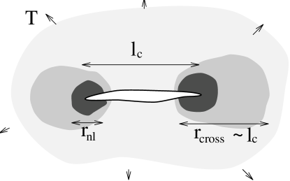
FIG. 9.: In the crack system there are two well-defined zones: the outer zone, consisting of exclusively linear elastic material, and the inner, crack tip zone where the nonlinear processes take place. Such separation introduces two length scales: the first $(r_{\rm nl})$ determines the size of the nonlinear zone, and the second $(r_{\rm cross})$ gives the scale where the elastic fields near the crack tip deviate from the ones predicted by SSY to comply with the outer zone boundary conditions.

First, let’s consider the energy in the nonlinear zone. The saddle point energy is $\alpha\ell_{c}$ and diverges as $1/T^{2}$ as $T\to 0$, while the elastic energy in the nonlinear zone $E_{\rm nl}$ is bounded by the linear value

$$E_{\rm nl}\sim\int_{0}^{r_{\rm nl}}dr\ r\sigma_{ij}^{2}(r)/Y\sim\alpha^{2}/Y.$$ (256)

Since $E_{\rm nl}$ is fixed as $T\to 0$, it renormalizes $n_{0}$ in (234) and hence does not affect the asymptotics (253).

Second, we consider how the existence of the inner (nonlinear) zone changes the energy in the outer (linear) zone. The elastic equations around the crack tip allow many solutions[27]; in each, the stresses $\sigma_{ij}$ have the form $C_{b}r^{b}f_{b}(\theta)$, $r_{\rm nl}\ll r\ll r_{\rm cross}$, in polar coordinates $(r,\theta)$ centered at the crack tip, where $b$ is an half-integer, the $C_{b}$ are constants, and the $f_{b}$ are known trigonometric functions. Linear fracture mechanics predicts $b=-1/2$ to be the most singular solution (compare with (254)) only because modes with $b<-1/2$ would give rise to singular displacements at the crack tip. Incorporation of the nonlinear zone $r<r_{\rm nl}$ however, removes this constraint. In other words, the nonlinear zone introduces new boundary conditions for linear elasticity solutions, allowing them to be more singular. The dominance of $b=-1/2$ solution is known as small scale yielding (SSY) approximation. Analyzing the mode III anti-plane shear fracture, Hui and Ruina argued[28] that SSY approximation becomes more and more accurate as $\epsilon=r_{\rm nl}/r_{\rm cross}\to 0$. (They expect that the same result can be extended for mode I fracture.) Clearly, in our case $\epsilon\to 0$ as $T\to 0$; thus the dominant contribution still comes from $b=-1/2$ solution. In fact, following [27] we expect

$$\sigma_{ij}\{C_{n}\} = T\biggl{(}C_{-1/2}\sqrt{{\ell_{c}}\over{r}}$$ (259)

$$+\sum_{n=\{\cdots,\ -7/2,\ -5/2,\ -3/2\}}C_{n}{\biggl{(}{r\over{r_{\rm nl}}}\biggr{)}}^{n}$$

$$+\sum_{n=\{\ 1/2,\ 3/2,\ 5/2,\cdots\}}C_{n}{\biggl{(}{r\over{l_{c}}}\biggr{)}}^{n}\biggr{)}.$$

The inelastic stresses at the outer boundary of the nonlinear zone $r\sim r_{\rm nl}$ are of order $Y$, thus from (259), for $n<-1/2$, $C_{n}=O(\epsilon^{-1/2})$ (recall that $\epsilon=r_{\rm nl}/r_{\rm cross}\sim(T/Y)^{2}$). These more singular terms in turn generate corrections to $C_{n}$ with $n\geq 1/2$ of order $O(\epsilon)$. (One can see this from the fact that the dominant contribution from the more singular terms at $r\sim\ell_{c}$ is $C_{-3/2}({\ell_{c}}/r_{\rm nl})^{-3/2}\sim\epsilon$.) The dependence of $C_{n}$ in (259) on the polar angle $\theta$ is implied.

There is a formal analogy between the arguments presented here for the stress fields in the crossover zone with the quantum mechanical problem of the bound states of the hydrogen atom. When we treat hydrogen nucleus as a point charge, for each orbital quantum number, the electron wave function has two solutions near the origin (the position of the nucleus): one is finite as $r\to 0$ and the other one is divergent[29, 30]. In a point charge problem one immediately discards the divergent solution because it can not be normalized and thus can not represent a bound state. However, in a finite-size nucleus model one notices that the electron wave function outside the nucleus is a mixture of the finite and the divergent solutions of the point charge problem. The normalization is resolved because inside the nucleus the electron wave function satisfies a different equation and becomes finite. The radius of the nucleus serves as a short-distance cutoff similar to $r_{\rm nl}$ in the crack problem.

The change in the contribution to the saddle point energy from the outer zone as a result of the introduction of the nonlinear zone, $\delta E_{\rm outer}$, is given by

$$\delta E_{\rm outer}\sim\int_{r_{\rm nl}}^{\ell_{c}}dr\ r{{\sigma_{ij}^{2}\{C_{n}\}-\sigma_{ij}^{2}\{C_{n}^{\rm linear}\}}\over Y}.$$ (260)

The dominant contribution to (260) comes from the cross term between $n=-1/2$ and $n=-3/2$ corrections in (259):

$$\delta E_{\rm outer}\sim{{\alpha^{2}}\over Y}\ln{{T\over Y}}:$$ (261)

the correction renormalizes the $n_{1}$ coefficient in the imaginary part of the free energy (LABEL:185) (regularization dependent in a first place), leaving the asymptotic ratio (253) intact.

It is no surprise that the nonlinear effects do not change the generic form of the imaginary part (LABEL:185). The detailed nonlinear description of the crack tips is a specification of the ultraviolet (short scale) physics and thus is nothing but another choice of the regularization. From our experience with $\zeta$-function and the lattice regularizations, we naturally expect that this nonlinear regularization preserves the form of the imaginary part (LABEL:185).

Finally, let’s consider the enhanced nucleation of secondary cracks in the high-strain outer-zone region — a possible cause for breakdown of the “dilute gas” approximation. Inside the nonlinear zone of the saddle point crack, the critical crack length for a second crack is of the order $\alpha/Y$ ( from (129) with $T\sim Y$ ) and thus such microcracks can be easily created. In fact, the nucleation of these microcracks may well be the dominant mechanism of the main crack propagation. Micro-crack nucleation in the nonlinear zone will change the stress fields near the crack tips, but as we discuss above, has little impact on the saddle point energy (as the total energy in the nonlinear zone is finite). We show now that such secondary crack nucleation is exponentially confined to the nonlinear zone of the main crack. The probability $W(r_{0})$ of the second crack nucleated somewhere at $r>r_{0}\sim r_{\rm nl}$ ($r=0$ corresponds to a crack tip) is given by

$$W(r_{0})\sim\int\limits_{r_{0}}^{+\infty}{{rdr}\over{\lambda^{2}}}\exp\{-\beta\alpha\ell(r)\}$$ (262)

where $\ell(r)$ is a critical crack length at distance $r$ from the tip of the critical crack. From (129) with $T$ replaced with the stress field near the crack tip given by (254), we find

$$\ell(r)\sim{{\alpha Y}\over{{\sigma_{ij}(r)}^{2}}}\sim r$$ (263)

(262) with (263) gives

$$W(r_{0})\sim\int\limits_{r_{0}}^{+\infty}{{rdr}\over{\lambda^{2}}}\exp\{-\beta\alpha r\}={{1+\beta\alpha r_{0}}\over{{(\beta\alpha\lambda)}^{2}}}\exp\{-\beta\alpha r_{0}\}$$ (264)

The exponential dependence of $W(r_{0})$ on the boundary of the nonlinear zone $r_{0}\sim r_{nl}$ in equation (264) means that the nucleation of another crack (in addition to the saddle point one) is exponentially confined to the nonlinear zone, justifying the dilute gas approximation.

VII Other geometries, stresses, and fracture mechanisms

In this section we discuss generalizations of our model, more exactly its simplified version without the quadratic fluctuations. We will do five things. In (A) we calculate the imaginary part of the free energy for arbitrary uniform loading and find the high-order nonlinear corrections to Young’s modulus. We discuss the effects of dislocations and vacancy clusters (voids) in (B) and (C). Part (D) deals with three dimensional fracture through the nucleation of penny-shaped cracks: we calculate the imaginary part of the free energy and the asymptotic ratio of the successive coefficients of the inverse bulk modulus. Finally, in (E) we consider a non-perturbative effect: the vapor pressure of a solid gas of bits fractured from the crack surfaces, and show how it affects the saddle point calculation.

A Anisotropic uniform stress and the high order corrections to Young’s modulus.

We calculated the essential singularity of the free energy at zero tension only for uniform isotropic loads at infinity. Within the approximation of ignoring the quadratic fluctuations, we can easily generalize to any uniform loading. In general, consider an infinite elastic material subject to a uniform asymptotic tension with $\sigma_{\rm yy}=T$, $\sigma_{\rm xx}=\epsilon T$ ($0\leq\epsilon<1$) and $\sigma_{\rm xy}=0$. Using the strain-stress analysis of[17] and following (28)-(31), we find the energy $E_{\rm release}$, released from the creation of the straight cut of length $\ell$ tilted by angle $\theta$ from the $x$ axis

$$E_{\rm release}={{\pi T^{2}\ell^{2}(1+\chi)}\over{64\mu}}\biggl{[}(1+\epsilon)+(1-\epsilon)\cos 2\theta\biggr{]}.$$ (265)

(The isotropic result (2) is restored for $\epsilon=1$.) The new important feature that comes into play is that the crack rotation ceased to be a zero-restoring-force mode. Treating the crack rotation to quadratic order in $\theta$ from the saddle point value $\theta=0$, we obtain the total energy of the crack $E(\Delta\ell,\theta)$ similar to (128-130), (133)

$$E(\Delta\ell,\theta)=\alpha\ell_{c}-{{\alpha\Delta\ell^{2}}\over{\ell_{c}}}+\alpha\ell_{c}(1-\epsilon)\theta^{2}.$$ (266)

As before, $\Delta\ell$ is the deviation of the crack length from the saddle point value $\ell_{c}$, still given by (129). Following (135)-(140), the imaginary part of the free energy for a dilute gas of straight cuts, excluding all quadratic fluctuations except for the uniform contraction-expansion (mode $\Delta\ell$) and the rotation (mode $\theta$) of the critical droplet, is given by

$${\rm Im}F^{\rm simple}(T,\epsilon) = \pm{\pi\over{2\beta^{2}\alpha\lambda}}\biggl{(}{{{A}\over{\lambda^{2}}}}\biggr{)}{\biggl{(}{1\over{1-\epsilon}}\biggr{)}}^{1/2}$$ (268)

$$\exp{\biggl{\{}{{-32\beta\mu\alpha^{2}}\over{\pi T^{2}(\chi+1)}}\biggr{\}}}.$$

One immediately notices an intriguing fact: the $\epsilon$-dependence of the imaginary part is only in the prefactor, which, as we already know is regularization dependent anyway. In particular, the latter means that the inverse Young’s modulus — the elastic coefficient corresponding to the transition with path $\epsilon=0$ — will have the same asymptotic behavior as that of the inverse bulk modulus (253): the asymptotic ratio of the high-order elastic coefficients of the inverse Young’s modulus $Y(P)$

$${1\over Y(P)} = -{1\over A}\left({\partial A\over\partial P}\right)_{\beta}=Y_{0}+Y_{1}P\cdots+Y_{n}P^{n}+\cdots$$ (269)

($P$ in (269) is a uniaxial compression) are given by

$${{Y_{n+1}}\over{Y_{n}}}\to-n^{1/2}{\biggl{(}{{\pi(\chi+1)}\over{64\beta\mu\alpha^{2}}}\biggr{)}}^{1/2}\mbox{\hskip 7.22743pt as {\it n}}\rightarrow\infty.$$ (270)

B Dislocations

We have forbidden dislocation nucleation and plastic flow in our model. Dislocation emission is crucial for ductile fracture, but by restricting ourselves to a brittle fracture of defect–free materials we have escaped many complications. Dislocations are in principle important: the nucleation[31] barrier $E_{\rm dis}$ for two edge dislocations in an isotropic linear–elastic material under a uniform tension $T$ with equal and opposite Burger’s vectors $\vec{b}$ is

$$E_{\rm dis}={{Yb^{2}}\over{4\pi(1-\sigma^{2})}}\ln{Y\over T}+E_{0}$$ (271)

where $E_{0}$ is a $T$ independent part that includes the dislocation core energy. The fact that $E_{\rm dis}$ grows like $1/\ln T$ as $T\to 0$ (much more slowly than the corresponding barrier for cracks) tells that in more realistic models dislocations and the resulting plastic flow[32] cannot be ignored. While dislocations may not themselves lead to a catastrophic instability in the theory (and thus to an imaginary part in the free energy?), they will strongly affect the dynamics of crack nucleation (e.g., crack nucleation on grain boundaries and dislocation tangles)[14, 26].

C Vacancy clusters

We ignore void formation. It would seem natural to associate the negative pressure (tension) $(-T)$ times the unit cell size with the chemical potential $\mu$ of a vacancy. At negative chemical potentials, the dominant fracture mechanism becomes the nucleation of vacancy clusters or voids (rather than Griffith-type microcracks), as noted by Golubović and collaborators[33]. If we identify the chemical potential of a vacancy with $-T$, we find the total energy of creation a circular vacancy of radius $R$, $E_{\rm vac}(R)$, to be

$$E_{\rm vac}(R)=2\pi R\alpha-T\pi R^{2}.$$ (272)

From (272) the radius of the critical vacancy is $R_{c}=\alpha/T$ and its energy is given by $E_{\rm vac}(R_{c})=\pi\alpha^{2}/T$. A saddle point is a circular void because a circular void gains the most energy ($\sim$ area of the void) for a given perimeter length. In principle, the exact shape of the critical cluster is also affected by the elastic energy release. The latter, however,

$$E_{\rm release}(R_{c})={{\pi T^{2}R_{c}^{2}(3\chi+1)}\over{8\mu}}={{\pi\alpha^{2}(3\chi+1)}\over{8\mu}}$$ (273)

is fixed as $T\to 0$, and thus the energy of the vacancy is dominated by $E_{\rm vac}(R_{c})$ for small $T$. (To obtain (273) we used the strain-stress analysis of[17] and expression (31) for the energy release.) Using the framework developed for the crack nucleation, we find that in case of voids (again, ignoring the positive frequency quadratic fluctuations) the imaginary part of the free energy is given by

$${\rm Im}F^{\rm simple}_{\rm vacancy}(T)=\pm{1\over{2\beta}}\biggl{(}{{{A}\over{\lambda^{2}}}}\biggr{)}{\biggl{(}{1\over{\beta T\lambda^{2}}}\biggr{)}}^{1/2}\exp{\biggl{\{}{{-\pi\beta\alpha^{2}}\over T}\biggr{\}}}.$$ (274)

(The special feature of the calculation (274) is that translations are the only zero modes: the rotation of a circular vacancy cluster does not represent a new state of the system.) From (274) we obtain following (244) and (247) the asymptotic ratio of the high-order coefficients of the inverse bulk modulus

$${{c_{n+1}}\over{c_{n}}}\to-{n\over{\pi\beta\alpha^{2}}}.$$ (275)

The divergence of the inverse bulk modulus is much stronger in this case: the high-order coefficients grow as $c_{n}\sim n!$, rather than as $(n/2)!$ (for the fracture through the crack nucleation).

Whether (275) is a realistic result is an open question. Fracture through vacancy cluster nucleation is an unlikely mechanism for highly brittle materials: the identification of $\mu$ with $(-T)$ demands a mechanism for relieving elastic tension by the creation of vacancies. The only bulk mechanism for vacancy formation is dislocation climb, which must be excluded from consideration — the dislocations in highly brittle materials are immobile[26]. Vacancy clusters might be important for the fracture of ductile (non-brittle) materials. However, the nucleation of vacancies must be considered in parallel with the nucleation of dislocations. Because at small $T$ dislocations are nucleated much more easily (271) than vacancy clusters at low stresses, the dominant bulk mode of failure is much more likely to be crack nucleation at a dislocation tangle or grain boundary — as indeed is observed in practice.

D Three dimensional fracture

Our theory can be extended to describe a three dimensional fracture transition as well. Studying elliptical cuts, Sih and Liebowitz[11] found that a penny-shaped cut in a three-dimensional elastic media subject to a uniform isotropic tension $T$ relieves the most elastic energy for a given area of the cut. The energy to create a penny-shaped cut of radius $R$, $E_{\rm penny}(R)$, is given by[11]

$$E_{\rm penny}(R)=2\pi\alpha R^{2}-{{4(1-\sigma)R^{3}T^{2}}\over{3\mu}}.$$ (276)

The zero modes contribute in this case a factor $2\pi V/\lambda^{3}$ — $2\pi$ coming from the distinct rotations of the cut, and $V/\lambda^{3}$ coming from the translations of the cut. Here we find the imaginary part of the free energy to be

$${\rm Im}F^{\rm simple}_{\rm penny}(T) = \pm{1\over{2\beta}}\biggl{(}{2\pi{V\over{\lambda^{3}}}}\biggr{)}{\biggl{(}{1\over{2\beta\alpha\lambda^{2}}}\biggr{)}}^{1/2}$$ (278)

$$\exp{\biggl{\{}{{-2\beta\mu^{2}\pi^{3}\alpha^{2}}\over{{3(1-\sigma)}^{2}T^{4}}}\biggr{\}}}$$

and the asymptotic ratio of the high-order elastic coefficients of the inverse bulk modulus

$${{c_{n+1}}\over{c_{n}}}\to-{\biggl{(}{{{3(1-\sigma)}^{2}}\over{2\beta\mu^{2}\pi^{3}\alpha^{2}}}\biggr{)}}^{1/4}{\biggl{(}{n\over 4}\biggr{)}}^{1/4}.$$ (279)

E Vapor pressure

The approach we used to calculate the imaginary part of the free energy is a perturbative one. In a sense, nothing prohibits us from considering cubic, quartic, etc. deviations from the saddle point energy. In fact, it is possible to develop an analog of Feynman diagram technique (as in quantum electrodynamics[29] or quantum field theory[7]) and calculate the contribution to the imaginary part to any finite order. It is important to realize that even if we did this, the result would still be incomplete: we would miss interesting and important physics coming from nonperturbative effects. Here we discuss one such nonperturbative effect, namely the “vapor” pressure of a solid gas of bits fractured from the crack surface. We find that including the vapor pressure, the essential singularity shifts from $T=0$ to $T=-P_{\rm vapor}$. Consider a dilute gas of straight cuts of arbitrary length with an elliptical opening (mode $v_{1}$ in (118)) and a solid gas of fractured bits from the crack surface. Following[13], the partition function of the material with one cut $Z_{1}$ under a uniform isotropic tension $T$ is

$$Z_{1} = Z_{0}\biggl{(}\pi{A\over{\lambda^{2}}}\biggr{)}\int_{0}^{\infty}{{d\ell}\over{\lambda}}\int_{0}^{\infty}{{dv_{1}}\over{\lambda}}\exp\biggl{\{}-\beta\biggl{(}2\alpha\ell$$ (281)

$$+{{2\pi\mu}\over{\chi+1}}v_{1}^{2}-{{\pi T\ell}\over{2}}v_{1}\biggr{)}\biggr{\}}Z_{\rm gas}(\ell,v_{1}),$$

where $Z_{\rm gas}(\ell,v_{1})$ is the partition function of the gas of fractured bits inside the crack of area $\pi\ell v_{1}/2$. It costs $2\alpha\lambda$ to fracture one bit of size $\lambda\times\lambda$ from a crack step, so in an ideal gas approximation, the partition function of the gas is determined by

$$Z_{\rm gas}(\ell,v_{1}) = \sum_{n=0}^{\infty}\exp(-2\beta\alpha\lambda N){\biggl{(}{{\pi\ell v_{1}}\over{2\lambda^{2}}}\biggr{)}}^{N}{1\over{N!}}$$ (282)

$$= \exp\biggl{\{}{{\pi\ell v_{1}}\over{2\lambda^{2}}}\exp(-2\beta\alpha\lambda)\biggr{\}}.$$ (283)

From (281) and (282) it follows that the partition function of the gas effectively increases the tension $T$ by the vapor pressure $P_{\rm vapor}$, $T\to T+P_{\rm vapor}$, where

$$P_{\rm vapor}={1\over{\beta\lambda^{2}}}\exp(-2\beta\alpha\lambda).$$ (284)

In particular, the essential singularity of the free energy shifts from zero tension to minus the “vapor” pressure. This shift is clearly a nonperturbative effect. We were able to describe it only by allowing topologically different excitations in the system: a state of the elastic material with a bit completely detached from the crack surface may not be obtained by the continuous deformation of the crack surface (surface phonons) or the cut shape (curvy cuts). At zero external pressure, our material is in the gas (fractured) phase — not until $P_{\rm vapor}$ is the solid stable.

VIII Summary

In this paper we studied the stress-induced phase transition of elastic materials under external stress: an elastic compression “phase” under positive pressure goes to a fractured “phase” under tension. We showed that in a properly formulated thermodynamic limit, the free energy of an infinite elastic material with holes of predetermined shapes is independent of the shape of the outer boundary as the latter goes to infinity. Under a stretching load the free energy develops an imaginary part with an essential singularity at vanishing tension. To calculate the essential singularity of the free energy including quadratic fluctuations we determined the spectrum and normal modes of surface fluctuations of a straight cut, and proved that under the uniform isotropic tension a curvy cut releases the same elastic energy (to cubic order) as the straight one with the same end-points. The imaginary part of the free energy determines the asymptotic behavior of the high-order nonlinear correction to the inverse bulk modulus[13]. We find that although the prefactor and the renormalization of the surface tension are both regularization dependent (once we include the quadratic fluctuations), the asymptotic ratio of the high-order successive coefficients of the inverse bulk modulus apparently is a regularization-independent result.

Within our model, the asymptotic ratio is unchanged by the inclusion of the nonlinear effects near the crack tips. We generalize the simplified model (without the quadratic fluctuations) to anisotropic uniform strain and calculated the asymptotic behavior of the high order nonlinear coefficients of the inverse Young’s modulus. We computed the imaginary part of the free energy (and the corresponding divergence of the high-order coefficients of the inverse bulk modulus) for the fracture mechanism through void nucleation which dominates at small external pressures: we argue that it may not occur in brittle fracture and should be preempted by dislocation motion in ductile fracture. We find that the simplified model applied to three-dimensional fracture predicts a $(n/4)!$ divergence of the nonlinear coefficients of the inverse bulk modulus.

Our results can be viewed as a straightforward extension to the solid-gas sublimation point of Langer [18, 19] and Fisher’s [3] theory of the essential singularities at the liquid-gas transition. Indeed, if we allow for vapor pressure in our model, then our system will be in the gas phase at $P=0$, as noted in section VII(E). The essential singularity we calculate shifts from $P=0$ to the vapor pressure. If we measure the nonlinear bulk modulus as an expansion about (say) atmospheric pressure, it should converge — but the radius of convergence would be bounded by the difference between the point of expansion and the vapor pressure.

REFERENCES

- [1] A. A. Griffith, Philos. Trans. Roy. Soc. London Ser. A 221 163 (1920).
- [2] C. E. Inglis, Trans. Inst. Naval Archit. 55 219 (1913).
- [3] M. E. Fisher, Physics 3 255 (1967). Recent work has shown that some first-order phase transitions can have power-law singularities: D. J. Bukman and J. J. D. Shore, J. Stat. Phys. 78 1277 (1995).
- [4] R. I. B Selinger, Z. Wang and W. M. Gelbart, Phys. Rev. A 43 4396 (1990) and references therein.
- [5] R. L. Smith, S. L. Phoenix, M. R. Greenfield, R. B. Henstenburg and R. E. Pitt Proc. R. Soc. Lond. A 388 353 (1983) and references therein; also Ken Burton, unpublished.
- [6] F. J. Dyson Phys. Rev. 85 631 (1952).
- [7] J. Zinn-Justin, “Quantum field theory and critical phenomena”, Oxford University Press, New York ( 1989).
- [8] H. F. Bueckner, J. App. Mech., Trans. ASME 80 1225 (1958).
- [9] J. R. Rice, “Mathematical analysis in the mechanics of fracture”, in Fracture (ed. H. Liebowitz) vol. 2, Academic Press, New York (1968).
- [10] J. N. Goodier, “Mathematical theory of equilibrium cracks”, in Fracture (ed. H. Liebowitz) vol. 2, Academic Press, New York (1968).
- [11] G. C. Sih and H. Liebowitz, “Mathematical theories of brittle fracture”, in Fracture (ed. H. Liebowitz) vol. 2, Academic Press, New York (1968).
- [12] N. Goldenfeld, “Lectures on phase transitions and the renormalization group”, Addison-Wesley Publishing Company, Advanced Book Program (1993).
- [13] A. Buchel and J. P. Sethna, Phys. Rev. Lett. 77 1520 (1996). Here, calculating the imaginary part of the free energy we incorrectly found the contribution from the zero-restoring-force modes. Because straight cuts tilted by and with respect to, say, the axis are identical, the correct contribution from rotations should be , rather than . This constant does not change the other results of the paper.
- [14] H. L. Ewalds and R. J. H. Wanhill, “Fracture mechanics”, Edward Arnold and Delftse Uitgevers Maatschappij, Delft (1984).
- [15] J. R. Rice, J. App. Mech., Trans. ASME 35 379 (1968).
- [16] I. S. Sokolnikoff, “Mathematical theory of elasticity”, McGraw-Hill Book Company, New York (1956).
- [17] N. I. Muskhelishvili, “Some basic problems of the mathematical theory of elasticity; fundamental equations, plane theory of elasticity, torsion and bending”, Groningen, P. Noordhoff (1963).
- [18] J. S. Langer, Ann. Phys. 41 108 (1967); see also N. J. Günther, D. A. Nicole and D. J. Wallace, J. Phys. A 13 1755 (1980).
- [19] J. S. Langer, Ann. Phys. 54 258 (1969).
- [20] I. Affleck, Phys. Rev. Lett. 46 388 (1981).
- [21] P. Ramond, “Field theory : a modern primer”, Reading, Mass. : Benjamin/Cummings Pub. Co., Advanced Book Program (1981).
- [22] I.S. Gradshteyn and I.M. Ryzhik, “Table of integrals, series, and products”, Academic Press, Boston (1994).
- [23] C. M. Bender and T. T. Wu, Phys. Rev. 184, 1231 (1969).
- [24] E. Breźin, J. C. Le Guillou and J. Zinn-Justin, Phys. Rev. D 15 1558 (1977).
- [25] G. Parisi, Phys. Lett. B 66 167 (1977).
- [26] B. R. Lawn and T. R. Wilshaw, “Fracture of brittle solids”, Cambridge University Press, Cambridge (1975).
- [27] J. A. Hodgdon and J. P. Sethna, Phys. Rev. B 47 4831 (1993); J. A. Hodgdon, “Three dimensional fracture : symmetry and stability”, PhD thesis, (1993).
- [28] C. Y. Hui and Andy Ruina, Int. J. Frac. 72 97 (1995). They consider both integer and half-integer corrections to the stress fields near the crack tips. Hodgdon and Sethna[27] found that only half-integer corrections are needed to describe the influence of the nonlinear zone. Hui and Ruina used an over-complete set of functions to describe the angular dependence of the stress fields.
- [29] A. I. Akhiezer and V. B. Berestetski, “Quantum electrodynamics”, Interscience Publishers, New York (1965).
- [30] I. Pomeranchuk and S. Smorodinsky, J. Phys. 9 97 (1945).
- [31] D. R. Nelson, Phys. Rev. B 18 2318 (1978).
- [32] Two-dimensional dislocation–mediated plastic flow is closely related to the problem of vortex nucleation and superflow decay in superfluid films: V. Ambegaokar, B. I. Halperin, D. R. Nelson, and E. D. Siggia, Phys. Rev. Lett. 40, 783 (1978); V. Ambegaokar, B. I. Halperin, D. R. Nelson, and E. D. Siggia, Phys. Rev. B 21, 1806 (1980); P. Minnhagen, O. Wetman, A. Jonsson, and P. Olsson, Phys. Rev. Lett. 74, 3672 (1995).
- [33] L. Golubović and A. Peredera, Phys. Rev. E 51 2799 (1995). They conclude with the interesting and apparently correct statement that voids smaller than the Griffith length can nonetheless grow and fracture the material.