The Poisson ratio of crystalline surfaces

Abstract

A remarkable theoretical prediction for a crystalline (polymerized) surface is that its Poisson ratio $\sigma$ is negative. Using a large scale Monte Carlo simulation of a simple model of such surfaces we show that this is indeed true. The precise numerical value we find is $\sigma\simeq-0.32$ on a $128^{2}$ lattice at bending rigidity $\kappa=1.1$. This is in excellent agreement with the prediction $\sigma=-1/3$ following from the self-consistent screening approximation of Le Doussal and Radzihovsky.

Crystalline surfaces have been studied extensively in recent years. Unlike one-dimensional polymers, which are always crumpled, non self-avoiding crystalline surfaces undergo a continuous phase transition from a high temperature crumpled phase to a low temperature flat phase [1, 2, 3]. The flat phase is characterized by long-range orientational order in the normals to the surface.

There are several experimental realizations of crystalline surfaces. Some, like suspended layers of graphite oxide in aqueous solution [4, 5] or polymerized adsorbed mono-layers, are chemical systems one can synthetize in the laboratory. There are also beautiful biological examples of such surfaces [6]: the cytoskeleton of erythrocytes (red blood cells) is composed of a network of nodes (actin oligomers) and links (spectrin tetramers). A typical skeleton is a triangulated network of roughly 70,000 plaquettes.

The crumpling transition and the flat phase of crystalline surfaces have been investigated numerically by several authors. The interested reader may consult the excellent reviews [7, 8]. Bowick et. al. have recently performed a large scale simulation of a triangulated crystalline surface with bending rigidity using free boundary conditions [9]. The largest surface simulated has 32,258 triangles. The equilibrium distribution is sampled using a Monte Carlo algorithm with a local Metropolis update. The action used has a simple Gaussian potential and a bending energy term:

$$\beta H=\sum_{\langle ij\rangle}(\vec{r}_{i}-\vec{r}_{j})^{2}-\kappa\sum_{\langle\alpha\beta\rangle}\vec{n}_{\alpha}\cdot\vec{n}_{\beta},$$ (1)

where $\vec{r}_{i}$ is the position of node $i$, $\vec{n}_{\alpha}$ is the unit normal to triangle $\alpha$ and $\kappa$ is the bending rigidity. For $\kappa>\kappa_{c}\simeq 0.79$ the system is in a flat phase and it behaves like a membrane with anomalous elasticity.

The flat phase is characterized by the scaling of the renormalized effective elastic constants $\lambda_{R}\sim\mu_{R}\sim q^{\eta_{u}}$ and of the bending rigidity $\kappa_{R}\sim q^{-\eta}$. The exponent $\eta$ can be determined from the scaling of the height-height correlation function ($\eta$ is related to the roughness exponent $\zeta=1-\eta/2$). The exponent $\eta_{u}$ determines the finite size scaling of the mean square phonon fluctuations.

We summarize the results of [9] in Table I. These results are compared to the analytical predictions obtained from an $\epsilon=4-D$ expansion (AL) [10, 11], a large-$d$ expansion [11, 12, 13] and a self-consistent screening approximation (LR) [14]. In this notation $D$ represents the dimensionality of the elastic manifold and $d$ is the dimensionality of the embedding space (for physical membranes $D=2$ and $d=3$.) Scattering experiments on the red blood cell skeleton give $\zeta\simeq 0.65(10)$ [6].

Table I: The scaling exponents.

	MC	AL	LR	Large-$d$
$\eta$	$\sim 0.62$	24/25	$0.81...$	2/3
$\eta_{u}$	0.50(1)	2/25	$0.36...$	2/3
$\zeta$	0.64(2)	13/25	$0.59...$	2/3

In addition to the anomalous scaling of the coupling constants, one of the most dramatic effects of fluctuations on crystalline surfaces is the prediction of a negative Poisson ratio $\sigma$. The Poisson ratio measures the in-plane transverse response of the surface when stress is applied in the longitudinal direction. It is defined to be positive for matter which shrinks in the $\hat{x}$-direction when stretched in the $\hat{y}$-direction.

Analytical calculations in the context of a self-consistent screening approximation (LR) [14] and an $\epsilon$ expansion (AL) [10] predict that for crystalline surfaces $\sigma$ is $-1/3$ (LR) and $-1/5$ (AL) respectively. The unusual sign of the Poisson ratio is a result of entropic suppression of the height fluctuations in a membrane under stress [15]. This effect is clearly demonstrated by crumpling a sheet of paper and pulling on two opposite corners: the sheet expands in the direction transverse to the applied strain [16, 17].

In this letter we demonstrate numerically that a crystalline surface, defined by Eq. (1), indeed has a negative Poisson ratio, and that it agrees with the prediction from [14]. We compare our result with previous numerical determinations of $\sigma$ [18]. We stress that this work extends the analysis of Monte Carlo data collected in [9], and we refer to it for the details of the simulations.

Consider an asymptotically flat elastic surface at thermal equilibrium. In the Monge gauge, its behavior is described by the partition function

$$Z[\sigma_{ij}]=\int[dr]^{3}\exp\left\{-\int d^{2}\varsigma\left[\frac{1}{2}\left(2\mu_{0}u^{2}_{ij}+\lambda_{0}u^{2}_{kk}\right)+\frac{\kappa_{0}}{2}(\nabla^{2}h)^{2}-\sigma_{ij}u_{ij}\right]\right\},$$ (2)

where $\varsigma$ is the intrinsic coordinate, $\mu_{0}$ and $\lambda_{0}$ are the bare Lamé coefficients and $\kappa_{0}$ is the bending rigidity. The stress tensor $\sigma_{ij}$ represents an external source linearly coupled to the system. The strain tensor $u_{ij}$, to linear order in $\vec{u}$, is related to $\vec{r}$ by

$$\vec{r} = \vec{s}+\vec{u}+\hat{z}h$$ (3)

$$u_{ij} = \frac{1}{2}(\partial_{i}u_{j}+\partial_{j}u_{i}+\partial_{i}h\partial_{j}h).$$ (4)

Here $\vec{s}$ is the rest (equilibrium) position of the surface, assumed to lie in the $x$–$y$ plane, and $h$ is the height of the surface above the reference plane.

The Poisson ratio can be defined in terms of correlation functions at zero external stress using linear response theory. Considering a diagonal (hydrostatic) stress, the derivation is straightforward and leads to

$$\sigma=-\frac{\langle u_{xx}\,u_{yy}\rangle_{c}}{\langle u_{yy}^{2}\rangle_{c}},$$ (5)

where the subscript $c$ indicates the connected part. Since the correlation functions are measured in the limit of zero external stress ($\sigma_{ij}=0$) the system is isotropic in the $x$–$y$ plane and

$$\langle u_{xx}^{2}\rangle_{c}=\langle u_{yy}^{2}\rangle_{c}.$$ (6)

For computational purposes it is convenient to express the strain tensor in terms of the tangent vectors $\vec{t}_{i}=\partial_{i}\vec{r}$. The index $i$ refers to the intrinsic coordinate system. The strain tensor is

$$u_{ij}=\partial_{i}\vec{r}\cdot\partial_{j}\vec{r}-\langle\partial_{i}\vec{r}\rangle\cdot\langle\partial_{j}\vec{r}\rangle=g_{ij}-\delta_{ij},$$ (7)

where $g_{ij}=\partial_{i}\vec{r}\cdot\partial_{j}\vec{r}$ is the induced metric, and we have rescaled the intrinsic coordinates so that $\langle g_{ij}\rangle=\delta_{ij}$. Substituting Eq. (7) in Eq. (5) we get

$$\sigma=-\frac{\langle g_{xx}\,g_{yy}\rangle_{c}}{\langle g^{2}_{yy}\rangle_{c}}.$$ (8)

In terms of a discretized surface the induced metric $g$ assumes a simple form. Take for example the $xx$ component at point $\varsigma$

$$g_{xx}(\varsigma)=\partial_{x}\vec{r}_{\varsigma}\cdot\partial_{x}\vec{r}_{\varsigma}=(\vec{r}_{\varsigma+x}-\vec{r}_{\varsigma})\cdot(\vec{r}_{\varsigma+x}-\vec{r}_{\varsigma}),$$ (9)

which is the squared length of the “link” between the point at $\varsigma$ and its neighbor in the $\hat{x}$ direction.

The derivation of $\sigma$ implicitly assumed that the intrinsic coordinate system is orthogonal. As our discretized surface is a triangular lattice, we need to transform the coordinate system. In fact, we can directly access only the $\partial_{i}\vec{r}_{\varsigma}$, $i$ = 1, 2, 3, of Eq. (9), in the three natural directions of the triangular lattice, while Eq. (8) is expressed in terms of $\hat{x}$ and $\hat{y}$. If $\hat{e}_{1}$, $\hat{e}_{2}$, $\hat{e}_{3}$ are the basis vectors of a triangular lattice, we define the $\hat{x}$ direction to overlap with $\hat{e}_{1}$, and we use $\hat{y}=(\hat{e}_{2}+\hat{e}_{3})/\sqrt{3}$.

At this point we can use Eq. (6), isotropy, as a consistency check on our definition of the strain fluctuation. In fact we verified that $\langle g^{2}_{xx}\rangle_{c}$, $\langle g^{2}_{11}\rangle_{c}$, $\langle g^{2}_{22}\rangle_{c}$, $\langle g^{2}_{33}\rangle_{c}$, and $\langle g^{2}_{yy}\rangle_{c}$ are equal within numerical accuracy.

One can find an equivalent definition of $\sigma$ in terms of different correlation functions. Since $\langle g_{xx}g_{xx}\rangle_{c}-\langle g_{xx}g_{yy}\rangle_{c}=2\langle g_{xy}g_{xy}\rangle_{c}$ [18], it is easy to show that

$$\sigma=-1+2\frac{\langle g_{xy}g_{xy}\rangle_{c}}{\langle g_{xx}^{2}\rangle_{c}}.$$ (10)

We have verified that this definition gives results consistent with Eq. (8). But it must be noted that it is more difficult to use numerical methods to determine $\sigma$ from Eq. (10) as $\langle g_{xy}\rangle$ is much smaller than $\langle g_{xx}\rangle$.

Table II: The Poisson Ratio.

$L$	$\kappa=1.1$	$\kappa=2.0$
32	$-0.28(1)$	$-0.25(1)$
46	$-0.30(2)$	$-0.26(2)$
64	$-0.30(3)$	$-0.28(3)$
128	$-0.32(4)$	—

We report in Table II the measured values of the Poisson ratio for various sizes of the surface and for two different values of the bending rigidity $\kappa$. The errors quoted in the table are due to statistical fluctuations and are estimated using the binning method. In Figure 1 we plot $\sigma$ for $\kappa=1.1$. We see marked changes in $\sigma$ as the lattice size increases and as the bending rigidity increases. These discrepancies are a measure of the uncertainty in our determination of the Poisson ratio. We remark that theoretical arguments [10, 14] indicate that the behavior in the whole flat phase is governed by an infrared-stable fixed point at $\kappa=\infty$ (the fluctuations stiffen the surface at long wavelength). Hence we expect to find the correct asymptotic behavior as $L\to\infty$ anywhere above the crumpling transition. Larger values of the bending rigidity influence the results since the auto-correlation times are longer — it is more time consuming to gather the equivalent number of independent configuration. For both values of $\kappa$ the results are consistent with an approach to a value of $\sigma\sim-0.32$, which agrees with the theoretical prediction of $-1/3$ (LR). The infinite volume value is extracted from the fit to $\sigma(L)=\sigma(\infty)+{a(\kappa)}/{L^{b}}$. The statistical errors on the data do not allow for a reliable estimate of the exponent $b$.

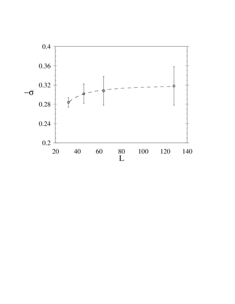
Figure 1: The Poisson ratio for $\kappa=1.1$ and $d=3L/4$.

Zhang, Davis and Kroll have obtained a different result $\sigma=-0.15(1)$ for the Poisson ratio of a tethered membrane in a molecular dynamics simulation with periodic boundary conditions [18]. There are several possible explanations for the discrepancy. We stress that the present simulation goes to much larger lattice sizes: in view of the finite size effects demonstrated in Table II, we believe size to be relevant. Furthermore, it is hard to compare the value of the bare parameters used in the two simulations because both the numerical techniques and the models studied differ.

For completeness we mention that Boal, Seifert and Shillcock have investigated numerically, and with mean field techniques, the Poisson ratio of 2-dimensional networks under tension [15]. These models differ from the one we study in that they are strictly planar. It was found, nonetheless, that entropic effects drive the Poisson ratio negative.

A comment now on our treatment of boundary effects. As noted by Abraham [19], large edge fluctuations might influence the results, even though boundary effects should vanish in the infinite volume limit. Zhang, Davis and Kroll simulate a surface in a closed cell [18], imposing periodic boundary conditions in the $x$–$y$ plane only, and, in some cases, dynamically modifying the cell size. In our simulations the surface’s boundary is free to fluctuate, and we need to carefully analyze the data in order to quantify the effect of boundary fluctuations. To this end, we restrict the definition of the correlation functions in Eq. (8) to a hexagonal subset of the mesh (the method is described in great detail in ref. [9]). The subset excludes the portions of the surface close to the boundary. For each size simulated ($L=32$, 46, 64, and 128) we construct 14 hexagonal regions of increasing diameter centered with respect to the bulk lattice. We then measure the correlation functions (and hence $\sigma$) restricted to these subsets. We found that, within our statistical error, the Poisson ratio for a subset of diameter $d$ is in fair agreement with the one of an independent surface of size $L=d$. Thus we conclude that $\sigma$ does not suffer much from boundary effects: presumably these effects cancel out in taking the ratio of the correlation functions. The values quoted in Table II are measured on subsets of diameter $d=3L/4$. The justification for this choice of subset size is given in [9]. We show there that the scaling exponents are insensitive to $d$ for subsets with $d\sim 3L/4$. Our choice is a compromise between excluding the boundary and including enough bulk surface for self-averaging. In Figure 2 we show the Poisson ratio for $L=46$ measured on the 14 subsets.

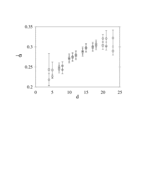
Figure 2: The Poisson ratio for the 14 subsets at $\kappa=1.1$ and $L=46$. The circles correspond to definition Eq. (8), while the squares to definition Eq. (10).

Details of the statistics gathered for the various lattice sizes and different bending rigidities are reported in [9]. For the largest lattices we ran $74\times 10^{6}$ Monte Carlo sweeps equivalent to 150 independent configurations. One sweep corresponds to a Metropolis update of each node of the lattice.

We acknowledge K. Anagnostopoulos, S. Catterall, G. Jungman, P. Le Doussal, D. Nelson, and L. Radzihovsky for helpful discussions and suggestions. NPAC has kindly provided computational facilities. The research of GT was sponsored by Syracuse University research funds for part of the work presented here. The research of MB and MF was supported by the Department of Energy U.S.A. under contract No. DE-FG02-85ER40237. EG thanks the S.U. Physics Department for their kind hospitality.

References

- [1] Y. Kantor and D. Nelson, Phys. Rev. Lett. 58, 1289 (1987).
- [2] R. Harnish and J. Wheater, Nucl. Phys. B 350, 861 (1991).
- [3] J. Ambjørn, B. Durhuus, and T. Jonsson, Nucl. Phys. B 316, 526 (1989).
- [4] X. Wen et al., Nature 355, 426 (1992).
- [5] T. Hwa, E. Kokufuta, and T. Tanaka, Phys. Rev. A 44, R2235 (1991).
- [6] C. F. Schmidt et al., Science 259, 952 (1993).
- [7] Fluctuating Geometries in Statistical Mechanics and Field Theory, edited by P. Ginsparg, F. David, and J. Zinn-Justin (Elsevier Science, Amsterdam, The Netherlands, 1996), “Les Houches Summer School Session LXII”.
- [8] Statistical Mechanics of Membranes and Surfaces, Vol. 5 of Jerusalem Winter School for Theoretical Physics, edited by D. Nelson, T. Piran, and S. Weinberg (World Scientific, Singapore, 1989).
- [9] M. J. Bowick et al., J. Phys. I (France) 6, 1321 (1996).
- [10] J. Aronovitz and T. Lubensky, Phys. Rev. Lett. 60, 2634 (1988).
- [11] J. Aronovitz, L. Golubović, and T. Lubensky, J. Phys. (France) 50, 609 (1989).
- [12] E. Guitter, F. David, S. Leibler, and L. Peliti, Phys. Rev. Lett. 61, 2949 (1988).
- [13] F. David and E. Guitter, Europhys. Lett. 5 (8), 709 (1988).
- [14] P. Le Doussal and L. Radzihovsky, Phys. Rev. Lett 69, 1209 (1992).
- [15] D. H. Boal, U. Seifert, and J. C. Shillcock, Phys. Rev. E 48, 4274 (1993).
- [16] D. R. Nelson, private communication.
- [17] P. Chaikin and T. Lubensky, Principles of condensed matter physics (Cambridge University Press, Cambridge, 1995).
- [18] Z. Zhang, H. T. Davis, and D. M. Kroll, Phys. Rev. E 53, 1422 (1996).
- [19] F. Abraham, Phys. Rev. Lett 67, 1669 (1991).