[

Sum rule for the optical Hall angle

Abstract

We consider the optical Hall conductivity of a general electronic medium and prove that the optical Hall angle obeys a new sum rule. This sum rule governs the response of an electronic fluid to a Lorentz electric field and can thought of as the transverse counterpart to the f-sum rule in optical conductivity. The physical meaning of this sum rule is discussed, giving a number of examples of its application to a variety of of electronic media.

]

The optical Hall conductivity is a new experimental probe.[1, 2] Like the optical conductivity, by extending Hall conductivity measurements into the microwave and far infrared, it should be possible to extract a host of new information about the properties of electronic systems in a magnetic field.[3] Electronic systems where this probe might prove particularly important, are the cuprate metals,[2] type II superconductors[4, 5] and the integer and fractional quantum Hall systems.[6]

One of the most useful tools in the experimental analysis of the optical conductivity, is the f-sum rule[7]

$$2\int_{0}^{\infty}{d\omega\over\pi}\sigma^{\prime}_{xx}(\omega)=\epsilon_{o}\omega_{p}^{2}$$ (1)

where $\sigma^{\prime}_{xx}(\omega)$ is the real part of the conductivity and $\omega_{p}$ is the plasma frequency. The distribution of optical spectral weight in an electronic medium gives us important information about its underlying physics. In this paper, we introduce a corresponding sum rule for the analysis of the optical Hall angle. The optical Hall angle, defined as

$${\rm tan}\theta_{H}(\omega)={\sigma_{xy}(\omega)/\sigma_{xx}(\omega)},$$ (2)

where $\sigma_{xx}$ and $\sigma_{xy}$ are the optical and Hall conductivities respectively, can be measured directly in optical transmission experiments.[1, 2] We shall show that this response function obeys the sum rule

$$2\int_{0}^{\infty}{d\omega\over\pi}{\rm tan}\theta_{H}^{\prime}(\omega)=\omega_{c},$$ (3)

where $\omega_{c}=eB/m$ is the cyclotron frequency of free electrons. Whereas the f-sum rule governs the longitudinal response to an applied electric field, this sum rule governs the transverse response to a Lorentz force. The transverse sum rule (3) will be refered to as the “t-sum” rule. The behaviour of the transverse spectral weight is, in general, independent of the longitudinal spectral weight: we shall see how this enables us to make a new, qualitative distinction between normal metals, superconductors, cuprate metals and quantum Hall systems.

The optical Hall angle extends the concept of a Hall angle to include retardation. In linear response theory, an input current $j_{y}$ leads to the retarded Hall current in the $x$ direction, $j_{x}$(Fig. 1. ) as follows

$$j_{x}(t)=\int^{t}_{-\infty}dt^{\prime}{\rm tan}\Theta_{H}(t-t^{\prime})j_{y}(t^{\prime}),$$ (4)

where ${\rm tan}\Theta_{H}(t)\equiv{\rm tan}\Theta_{H}^{(R)}(t)$ is the retarded Hall response function.

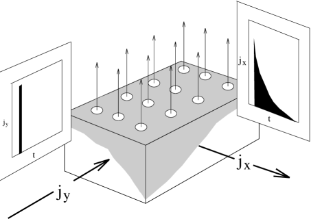
FIG. 1.: Illustrating the Hall response $j_{x}(t)=j_{o}{\rm tan}\Theta_{H}(t)$ to an input current pulse $j_{y}(t)=j_{o}\delta(t)$. In this thought experiment, the transverse electric field $E_{x}$ is constrained to be zero.

Our derivation leans heavily on the analytic properties of ${\rm tan}\theta_{H}(\omega)$, which we now discuss. Since ${\rm tan}\Theta_{H}(t)$ is a causal response function, it vanishes for negative times. General considerations tell us that its Fourier transform ${\rm tan}\theta_{H}(\omega)$, is analytic in the upper-half complex plane and satisfies the Kramer’s Krönig relations.[8]

$$\tan\theta_{H}(\omega+i\delta)=\int{dx\over\pi i}{1\over(x-\omega-i\delta)}\times\left\{\begin{array}[]{rl}i\rm tan\theta_{H}^{\prime\prime}(x)\cr\rm tan\theta_{H}^{\prime}(x)\end{array}\right.$$ (7)

The extension of these two expressions into the lower-half plane describe two different Riemann sheets of the function, and we must select the physical sheet that correctly describes retarded and advanced response functions as follows:

$${\rm tan}\Theta_{H}^{(R,A)}(t)=\int{d\omega\over 2\pi}{\rm tan}\theta_{H}(\omega\pm i\delta)e^{-i\omega t}.$$ (8)

Since $\sigma^{(R)}_{xx}(t)=-\sigma^{(A)}_{xx}(-t)$ and $\sigma^{(R)}_{xy}(t)=\sigma^{(A)}_{xy}(-t)$ are respectively odd and even under time-reversal, ${\rm tan}\theta_{H}=\sigma_{xy}\otimes\sigma_{xx}^{-1}$ is odd under time-reversal. Taking the Fourier transform (8), it follows that ${\rm tan}\theta_{H}(\omega)^{*}=-{\rm tan}\theta_{H}(\omega^{*})$, i.e, the physical Riemann sheet has a cut along the real axis where only the real-part of ${\rm tan}\theta_{H}(\omega)$ changes sign. The extension of the second Kramer’s Krönig relation ( 7) into the complex plane

$${\rm tan}\theta_{H}(z)=\int_{-\infty}^{\infty}{d\omega\over\pi i}{1\over\omega-z}{\rm tan}\theta_{H}^{\prime}(\omega).$$ (9)

provides the Riemann sheet that is consistent with this branch-cut structure. This spectral representation for the Hall angle holds on general grounds, even though we do not have an explicit Kubo formula for the Hall angle.

We now present a physical derivation of the t-sum rule. Suppose a small current pulse $j_{y}(t)=j_{o}\delta(t)$ is applied to the system. During the pulse, the current will precess at a rate $\omega_{c}$ about the magnetic field. The important point here, is that provided the pulse is brief enough, interactions and band-structure effects are negligible, precession is determined by the free-field Hamiltonian $H_{o}$, so that

$$\dot{\vec{j}}=i[H_{o},\vec{j}]=-\omega_{c}\hat{z}\times\vec{j},$$ (10)

where $\hat{z}$ is the direction of the magnetic field. The transverse Hall current that builds up during the pulse is

$$j_{x}(0^{+})=\omega_{c}\int_{0^{-}}^{0^{+}}dtj_{y}(t)=\omega_{c}j_{o}.$$ (11)

By (4), $j_{x}(0^{+})={\rm tan}\theta_{H}(0^{+})j_{o}$ so that

$${\rm tan}\theta_{H}(0^{+})=\omega_{c}=\int_{-\infty}^{\infty}{d\omega\over 2\pi}{\rm tan}\theta_{H}(\omega+i\delta)e^{-i\omega 0^{+}}$$ (12)

By extending this integral along an infinite semi-circular contour in the lower-half complex plane and deforming the contour onto the cut along the real axis, where ${\rm tan}\theta_{H}(\omega)$ has a discontinuity, the t-sum rule (3) follows.

A more general derivation follows from the Kubo formula. Let us take the magnetic field to lie along the z-direction, assuming the conductivity to be isotropic about this axis. The conductivity tensor in the basal plane can be written in the form $\sigma_{ab}(\omega)=Q_{ab}(\omega)/(-i\omega)$, ($a,\ b=x,y$) where in the time domain,

$$Q_{ab}(t)=\epsilon_{o}\omega_{p}^{2}\delta_{ab}\delta(t) - i\langle[\hat{j}_{a}(t),\hat{j}_{b}(0)]\rangle\theta(t).$$ (13)

The delta-function part is the instantaneous diamagnetic response, which is diagonal by inversion symmetry. The dominant short-time behavior of $Q_{ab}(t)$ is given by

$$\left.\begin{array}[]{rcl}Q_{xx}(t)&\sim&\epsilon_{o}\omega_{p}^{2}\delta(t),\cr Q_{xy}(t)&\sim&-i\langle[\hat{j}_{x},\hat{j}_{y}]\rangle\theta(t),\end{array}\right\}\qquad(t\rightarrow 0).$$ (16)

The Fourier transform of these expressions determine the asymptotic high frequency behavior of the conductivity tensor, so that

$$\begin{array}[]{rcl}\sigma_{xx}(z)&=&\displaystyle{\epsilon_{o}\omega_{p}^{2}/(-iz)},\cr\sigma_{xy}(z)&=&\displaystyle{i\langle[\hat{j}_{x},\hat{j}_{y}]\rangle/z^{2}},\end{array}\qquad\qquad(|z|\rightarrow\infty).$$ (19)

The asymptotic form of the Hall conductivity was previously obtained by Shraiman and Shastry, using a spectral decomposition.[3] Taking the ratio, we obtain ${\rm tan}\theta_{H}(z)=\omega_{H}/(-iz)$, ($|z|\rightarrow\infty$), where

$$\omega_{H}=\left({-i\langle[\hat{j}_{x},\hat{j}_{y}]\rangle\over\epsilon_{o}\omega_{p}^{2}}\right).$$ (20)

The Hall frequency, $\omega_{H}$ is the total residue of ${\rm tan}\theta_{H}(z)$ along the real axis. Multiplying the spectral representation ( 9) by $-iz$ and taking $|z|\rightarrow\infty$, we obtain

$$2\int_{0}^{\infty}{d\omega\over\pi}{\rm tan}\theta_{H}^{\prime}(\omega)=\omega_{H}.$$ (21)

For an electron gas with quadratic dispersion $-i[\hat{j}_{x},\hat{j}_{y}]=\omega_{c}(\omega_{p}^{2}\epsilon_{0}),$ so $\omega_{H}=\omega_{c}$. We will give a derivation of this result momentarily. Since all electronic systems are ultimately derived from a system with a quadratic dispersion, this is an exact result, but recovery of the full spectral weight requires an integration over all inter-band transitions. The usefulness of the sum rule derives from the fact that when the bands are well separated, an effective sum rule applies to the lowest band. Consider a single band described by the Hamiltonian

$$H[A]=\sum_{\vec{p}}\epsilon_{\vec{p}-e\vec{A}}\hat{n}_{\vec{p}},$$ (22)

where $\hat{n}_{\vec{p}}=\psi^{\dagger}_{\vec{p}}\psi_{\vec{p}}$ is the number operator. The plasma frequency of the band is given by

$$\epsilon_{o}\omega_{p}^{2}=\langle\nabla^{2}_{\vec{A}_{x}}H[A]\rangle=(e^{2}/2)\sum_{\vec{p}}{\rm Tr}(\underline{m}_{\rm\vec{p}}^{-1})n_{\rm\vec{p}}$$ (23)

where $[\underline{m}_{\rm\vec{p}}^{-1}]_{ab}=\nabla^{2}_{ab}\epsilon_{\rm\vec{p}}$ is the two-dimensional effective mass tensor and $n_{\vec{p}}=\langle\hat{n}_{\vec{p}}\rangle$. Provided that the magnetic flux per unit cell is far less than a flux quantum $h/e$, we may use a weak field approximation to $[\hat{j}_{x},\hat{j}_{y}]$, obtained by linearizing the velocity operator as follows

$$\vec{v}_{\vec{p}-e\vec{A}}=\vec{v}_{\vec{p}_{o}}+\underline{m}^{-1}_{\vec{p}}({{\vec{p}\kern-4.73611pt\raise-0.86108pt\hbox{/}}}-\vec{p}_{o}),$$ (24)

where ${{\vec{p}\kern-4.73611pt\raise-0.86108pt\hbox{/}}}=\vec{p}-e\vec{A}$. Since $[{p\kern-4.73611pt\raise-0.86108pt\hbox{/}}_{x},{p\kern-4.73611pt\raise-0.86108pt\hbox{/}}_{y}]=-ieB_{z}$, it follows that $[\vec{v}_{x},\vec{v}_{y}]={(eB){\rm det}(\underline{m}_{\rm\vec{p}}^{-1})}$. Writing $\hat{j}=\sum\psi^{\dagger}_{\rm\vec{p}}\vec{v}_{{{\vec{p}\kern-3.31529pt\raise-0.60275pt\hbox{/}}}}\psi_{\rm\vec{p}}$, we obtain the operator identity

$$[\hat{j}_{x},\hat{j}_{y}]=\sum_{\vec{p}}\left({e^{3}B{\rm det}(\underline{m}_{\rm\vec{p}}^{-1})}\right)\hat{n}_{\vec{p}}+O(B^{3}).$$ (25)

Combining (23) and (25), it follows that

$$\omega_{H}={eB}{\sum_{\vec{p}}{\rm det}[\underline{m}^{-1}_{\vec{p}}]n_{\vec{p}}\over\frac{1}{2}\sum_{\vec{p}}{\rm Tr}[\underline{m}^{-1}_{\vec{p}}]n_{\vec{p}}}.$$ (26)

For a parabolic band, ( 26) reverts to the free cyclotron frequency $\omega_{c}=eB/m$. Since this expression is dominated by contributions far from the Fermi surface, the Hall frequency will be only weakly temperature dependent. Suppose the system possesses a Fermi surface where $n_{\rm p}=1$ far inside and $n_{\rm p}=0$ far outside. To extract the dominant contribution to $\omega_{H}$, we we may set $n_{\rm\vec{p}}=1$ and restricting the integrals within each Fermi surface sheet. Both integrands are total derivatives,

$${\rm det}[\underline{m}^{-1}_{\vec{p}}] = -\frac{1}{2}\nabla\times\bigl{[}(\nabla\vec{u})\times\vec{u}\bigr{]},$$ (27)

$${\rm Tr}[\underline{m}^{-1}_{\vec{p}}] = \nabla\cdot\vec{u},$$ (28)

where $\vec{a}\times\vec{b}=\epsilon_{\alpha\beta}a_{\alpha}b_{\beta}$ denotes the two-dimensional cross-product, $\vec{u}$ denotes the component of the group velocity in the x-y plane and $(\nabla\vec{u})_{ab}=\underline{\rm m}^{-1}_{ab}$. This enables us to re-write the t-sum rule as a ratio of Fermi surface integrals.

$$\omega_{H}=eB{\int dp_{z}\int_{\rm FS}\vec{u}\times d\vec{u}\over\int dp_{z}\int_{\rm FS}d\vec{S}\cdot\vec{u}}+O(\delta\epsilon^{2}/\epsilon_{F}^{2}).$$ (29)

Here “FS” denotes a line integral around all sheets of the Fermi surface at constant $p_{z}$, $d\vec{S}$ denotes the surface increment that lies perpendicular to this line, $d\vec{u}=dk.\nabla\vec{u}$ is the change in $\vec{u}$ along the line and $\delta\epsilon/\epsilon_{F}$ is the ratio of the smearing of the Fermi surface to the Fermi energy. The numerator is readily identified as twice the area swept out by the Fermi velocity $\vec{u}$ around the Fermi surface. A variant of this expression has been obtained by Ong[9] using Boltzmann transport theory. Provided the Fermi surface is reasonably well-defined, we expect this expression to be robust.

We now illustrate the qualitative implications of the Hall sum rule using a few physical examples. In the case of a simple metal, the transverse optical conductivity in a magnetic field is given by

$$\sigma_{\pm}=\sigma_{xx}\pm i\sigma_{xy}={ne^{2}\over m}{1\over\Gamma_{tr}-i(\omega\mp\omega_{c})}$$ (30)

so that the optical conductivity is peaked at the cyclotron frequency. Remarkably, these poles do not enter the Hall response,

$${\rm tan}\theta_{H}(\omega)={\omega_{c}\over\Gamma_{tr}-i\omega},$$ (31)

which has the same form as the zero field optical conductivity (Fig. 2a). The Hall spectral weight is peaked at zero frequency and is independent of carrier density. In this case, the Hall constant $R_{H}(\omega)={\rm tan}\theta_{H}(\omega)/\sigma_{xx}(\omega)$ is frequency independent.

An intriguing exception to this behavior is found in the cuprate metals. Unlike conventional metals, transport measurements indicate that $\Gamma_{tr}\sim 2T$, but D.C. Hall measurements show that $[{\rm cot}\theta_{H}]\sim T^{2}$ is a quadratic function of temperature. Since the D.C. Hall angle scales as $1/T^{2}$, the sum rule tells us that the Hall relaxation rate $\Gamma_{H}$ is a quadratic function of tempterature $\Gamma_{H}=T^{2}/W$ and that furthermore $\sigma_{xy}\sim 1/(\Gamma_{tr}\Gamma_{H})$. This multiplicative combination of relaxation rates is unprecedented and does not fit into a conventional picture of normal metals. Based on this result, Anderson has conjectured that the Hall currents are subject to an autonomous decay process that depends quadratically on temperature $\Gamma_{H}\propto T^{2}$.[10] This controversial interpretation follows naturally from a Hall sum rule, in a fashion that is independent of the microscopic physics. A definitive measurement of the quadratic temperature dependence of the Hall decay rate would constitute a striking confirmation of the power of the Hall sum rule. (Fig. 2(b))

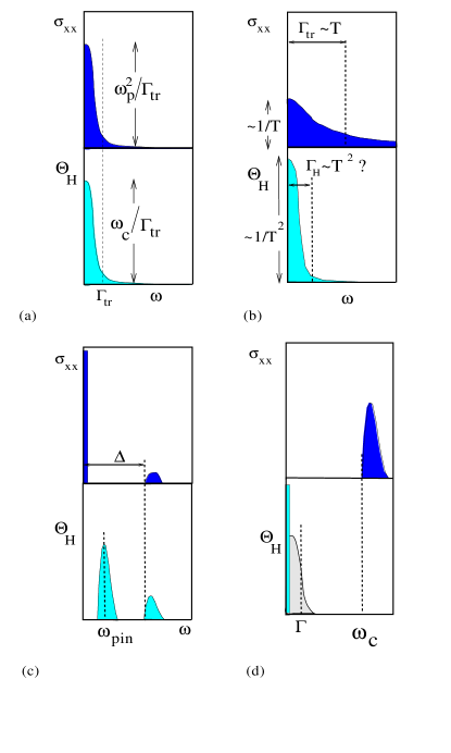
FIG. 2.: Contrasting the optical conductivity and the optical Hall angle in (a) a simple metal (b) a cuprate metal, (c) a superconductor and (d) a quantum Hall fluid. The superconductor displays condensation in the dynamical conductivity; the quantum Hall fluid displays displays a condensation in the optical Hall angle at a Hall plateau which periodically broadens into a Drude peak between plateaus.

As a second application, consider a type II superconductor with a pinned vortex lattice. In a superconductor, the optical conductivity condenses into a zero-energy delta function peak. However, the same condensation does not take place in the Hall angle, because unlike conventional currents, super-currents can not precess in a magnetic field: the deflection of a supercurrent requires a sideways movement of the flux lattice. Hsu[11] has computed the Hall response of a pinned flux lattice, and shown that it is shifted to the flux lattice pinning frequency (Fig. 2(c)), as observed in recent experiments on YBCO[12]. Pehaps the most important property of the sum rule in this respect, is that it does not depend on temperature or the thermodynamic state of the system. Despite the radically different physics of the vortex lattice and the normal state, the Hall sum is identical.

As a final example, we consider the Hall response of a two-dimensional electron gas in a high magnetic field. When the quantized, or fractionally quantized Hall ground-state develops, the conductivity ( 30) is qualitatively modified, leading to the quantum Hall effect in the D.C. response : ${\sigma_{xx}}=0$, $\sigma_{xy}=\nu e^{2}/h$, where $\nu=p/q$ is a rational number with an odd denominator. However, the oscillator strength sum rule is still dominated by the poles at $\omega_{c}$. What happens to the Hall angle? Like an insulating dielectric, the optical conductivity at a Hall plateau vanishes linearly with frequency $\sigma_{xx}(\omega)=\alpha(-i\omega)$ at $T=0$.[13] This implies that the a.c. Hall angle has the form

$${\rm tan}\theta_{H}(\omega)={1\over-i\omega}\left({\nu e^{2}\over h\alpha}\right)$$ (32)

i.e. the Hall angle response has condensed into a delta function. Assuming all the Drude weight condenses, then ${\rm tan}\theta_{H}(\omega)={\omega_{c}/(-i\omega)}$ and $\alpha$ takes its minimum value $\alpha=\nu e^{2}/h\omega_{c}$. From this qualitative reasoning, we clearly see how a quantum Hall system at $T=0$ is the transverse counterpart to a superconductor. In a superconductor, the longitudinal current accelerates in response to an electric field, but there is no Hall response. In a quantum Hall system, the transverse Hall current exhibits a superfluid response to a Lorentz electric field, but there is no longitudinal response. Between Hall steps, we expect the delta function to broaden into a Drude form of width $\sim\Gamma_{tr}$. At $T=0$ this occurs abruptly as a function of electron density or magnetic field, corresponding to a quantum phase transition. Therefore, we again see the analogy between the Hall angle in this system and and the change in the conductivity at a superconducting phase transition. At finite temperatures, $\sigma^{\prime}_{xx}\sim{e^{2}\over\hbar}e^{-E_{g}/{k_{B}T}}$, where $E_{g}$ is the gap in the density of states, so we expect the delta-function to broaden into a Lorentzian of width $\delta\omega\sim\nu\omega_{c}e^{-E_{g}/{k_{B}T}}$. The Hall angle sum rule should prove very useful in studies of the conductivity of quantum Hall systems, since it gives a spectral sum rule that may saturate at Frequencies $\omega\sim\Gamma_{tr}<<\omega_{c}$, which is the physically interesting range of frequencies.

In conclusion, we have considered the optical Hall angle as a dynamical response function, and showed that it obeys a sum rule that governs the evolution of transverse Hall currents. From our discussion of its qualitative application to metals, cuprate metals, BCS superconductors and quantized Hall systems, we see that the optical Hall angle may be thought of as the transverse analogue to the optical conductivity. Like the f-sum rule of the optical conductivity, the corresponding t-sum rule is independent of detailed microscopic physics, making it of great utility in the qualitative analysis of magneto-optic response of electronic systems.

We should like to thank R. Shankar, A. J. Schofield and S. C. Zhang for discussions related to this work. This work was supported in part by the National Science Foundation under Grants numbers DMR-93-12138, DMR-92-23217 and PHYS94-07194 during the course of a stay at the ITP, Santa Barbara.

REFERENCES

- [1] S. Spielman et al, Phys. Rev. Lett, 73, 1537 (1994).
- [2] S. G. Kaplan, S. Wu, H. T. S. Lihn and D. Drew, Q. Li, D. B. Fenner, Julia Phillips and S. Y. Hou, Phys. Rev. Lett. 76, 696 (1996).
- [3] B. S. Shastry, B. I. Shraiman and R. P. Singh, Phys. Rev. Lett 70 (2004), (1993).
- [4] A. Aronov, S. Hikami and A. I. Larkin, Phys. Rev. Lett. 64, 88 (1990).
- [5] G. Blatter, M.V. Feigelman, V. B. Gesgenbein, A. I. Larkin and V. M. Vinokur, Rev. Mod. Phys 66, 1125 (1994).
- [6] See for example, “The Quantum Hall Effect”, ed. R. E. Prange and S. M. Girvin (Springer Verlag, New York, 1987).
- [7] P. Nozières and D. Pines, Phys. Rev. 109, 741 (1958); F. Wooten, “Optical Properties of Solids” (Academic, New York , 1972).
- [8] E. M. Lifshitz and L. P. Pitaevskii, Statistical Mechanics vol. I, pp 377, Pergammon Press (1980).
- [9] N. P. Ong, Phys. Rev B43, 193 (1991).
- [10] P. W. Anderson, Phys. Rev. Lett. 67, 2092 (1991)
- [11] T. C. Hsu, Physica 213C . 305 (1993).
- [12] H. Lihn et al, Phys. Rev. Lett, 76, 3810 (1996).
- [13] This result follows from a Kramer’s-Krönig transformation of a function with a gap, it can also holds be inferred various works on the quantum Hall effect, see e.g C. Kallin and B. I. Halperin, Phys. Rev. B 31, 3635 (1985); S. Kivelson, D. H. Lee, S. C. Zhang, Phys. Rev B46, 2223 (1992).