“How should we interpret the two transport relaxation times in the cuprates ?”

Abstract

We observe that the appearance of two transport relaxation times in the various transport coefficients of cuprate metals may be understood in terms of scattering processes that discriminate between currents that are even, or odd under the charge conjugation operator. We develop a transport equation that illustrates these ideas and discuss its experimental and theoretical consequences.

]

“ There are and can exist but two ways of investigating and discovering truth. The one hurries on rapidly from the senses and particulars to the most general axioms, and from them, as principles and their supposed indisputable truth, derives and discovers the intermediate axioms. This way is now in fashion.

The other constructs its axioms from the senses and particulars, by ascending continually and gradually, till it finally arrives at the most general axioms. This is the true, but as yet untried way.”

Francis Bacon in “Novum Organum”, 1620

I Introduction.

One of the striking features of the cuprate metals, is the appearance of two, qualitatively different transport relaxation times. Resistivity and optical measurements indicate that electric currents relax at a rate which grows linearly[1] with temperature

$$\Gamma_{tr}\sim\eta T,\qquad(\eta\sim 2).$$ (1)

By contrast, the “Hall relaxation rate” obtained from the Hall angle[2] $\theta_{H}={\omega_{c}/\Gamma_{H}},$ where $\omega_{c}=eH/m$ is the cyclotron frequency, shows a qualitatively different quadratic temperature dependence

$$\Gamma_{H}={T^{2}\over W}+n_{i}b\;.$$ (2)

The quadratic form of $\Gamma_{H}$ is robust against a finite concentration of impurities $n_{i}$. Estimates of $W$ based on d.c. measurements by Ong et al., give $W\sim 1000K$, but more recent direct measurements of $\tau_{H}$ from the A.C. Hall angle, suggest that it may be significantly smaller. These features led Anderson, some five years ago, to conjecture that there are two transport relaxation times in the cuprate metals which independently govern the decay of electrical and Hall currents. [3, 4] Although subsequent experimental results have tended to reinforce this phenomenological interpretation, Anderson’s proposal remains highly controversial.

This article discusses the two-relaxation time conjecture. We sharpen the definition of the Hall and electric transport relaxation rate and show that a sum rule for the Hall angle means that Anderson’s interpretation can be made without reference to the microscopic physics. We explain why the robustness of the quadratic temperature dependence to changes in hole and impurity concentrations makes it very difficult to embrace the various alternative interpretations of the magneto-transport: the quadratic temperature dependence of $\Gamma_{H}$ appears there as a fortuitous cancelation of independent scattering processes.

Motivated by these considerations, we then pursue the consequences of the Anderson conjecture, bringing symmetry considerations into play.[5] We identify charge conjugation as the key symmetry distinction between the electric and the Hall currents, and argue that in the cuprates, there must be scattering processes involving the emission of charge that cause degenerate electron and hole states to admix in the normal state. These ideas are illustrated by a phenomenological transport equation. In the final section, we discuss the challenge of isolating the physics that simultaneously accounts for both the marginal scattering of the electrons and the delineation of electric and Hall currents.

II Review of Experimental results

The inverse-square Hall angle $\theta_{H}\sim T^{-2}$ is a robust feature of the cuprate metals which governs both the Hall conductivity and the magneto-resistance. Remarkably, the two relaxation times enter multiplicatively into the transport coefficients. The Hall conductivity $\sigma_{xy}=\sigma_{xx}\theta_{H}$ has the form

$$\sigma_{xy}\propto{H\over\Gamma_{tr}\Gamma_{H}},\qquad\qquad (\sim{T^{-3}})$$ (3)

where $H$ is the external field strength. In optimally doped cuprates, the magneto-conductivity $\Delta\sigma_{xx}$ depends quadratically on the Hall angle[6]

$$\Delta\sigma_{xx}\propto{H^{2}\over\Gamma_{tr}\Gamma_{H}^{2}},\qquad\qquad (\sim T^{-5})$$ (4)

In a normal metal there is one transport relaxation rate $\Gamma_{tr}(\vec{p})$ at each point in momentum space. $\Gamma_{tr}(\vec{p})$ can have strong momentum dependence, but since transport is a zero-momentum probe, momentum conservation prevents a multiplicative combination of scattering rates from different points on the Fermi surface. For example, the Hall conductivity of a Fermi liquid is given by the second moment of the transport relaxation time, around the Fermi surface

$$\sigma_{xy}\propto\int dp_{z}\int_{\rm FS}{\vec{v}\times d\vec{v}\over(\Gamma_{tr}(p))^{2}}\;,$$ (5)

where FS denotes a line integral around the Fermi surface in the plane perpendicular to the field, $\vec{v}$ is the Fermi velocity and $d\vec{v}=d\vec{p}\cdot\nabla\vec{v}$ is the change in $\vec{v}$ along the line.[7] Momentum conservation obliges us to interpret a multiplicative combination of $\Gamma_{tr}$ and $\Gamma_{H}$ in terms of two relaxation times at the same point in momentum space.

A clear manifestation of these two relaxation times, is the violation of Kohler’s rule. In conventional metals, where $\Gamma_{H}\sim\Gamma_{tr}$, the transverse magneto-resistance obeys Kohler’s rule $\delta\rho/\rho\propto(H/\rho)^{2}$.[8] Kohler’s rule is violated in the optimally doped and under-doped cuprate metals.[6] Instead, the appearance of the same Hall angle in the magneto-resistance means that a modified rule $\delta\rho/\rho\propto(H/\Gamma_{H})^{2}\propto(HR_{H}/\rho)^{2}$ is approximately satisfied.[9] Recent studies show that when the cuprate metals are over-doped, Kohler’s rule behavior is restored.[10]

To pursue this discussion, we need a clear idea of what we mean by the Hall and electric current relaxation rates. Electric current is the response to an applied electric field,

$$j_{x}(t)=\int_{-\infty}^{t}\sigma_{xx}(t-t^{\prime})E_{x}(t^{\prime})dt^{\prime}\;,$$ (6)

where $\sigma_{xx}(t-t^{\prime})$ is the Fourier transform of the frequency dependent conductivity. When we speak of a relaxation rate for the electrical current, we mean that the current response function $\sigma_{xx}(t-t^{\prime})$ has an exponential form

$$\sigma_{xx}(t-t^{\prime})={ne^{2}\over m}e^{-\Gamma_{tr}(t-t^{\prime})}\;,$$ (7)

This is the origin of the Drude peak in the optical conductivity. Hall current is the retarded transverse response to to an input current (Fig. 1 ) as follows

$$j_{x}(t)=\int_{-\infty}^{t}\Theta_{H}(t-t^{\prime})j_{y}(t^{\prime})dt^{\prime}\;,$$ (8)

where $\Theta_{H}(t)$ is the Fourier transform of the frequency dependent Hall angle $\theta_{H}(\omega)=\sigma_{xy}(\omega)/\sigma_{xx}(\omega)$. The Hall relaxation rate refers to the decay of the Hall current in response to a sudden pulse of current

$$\Theta_{H}(t-t^{\prime})=\omega_{c}e^{-\Gamma_{H}(t-t^{\prime})}\;,\qquad(t>t^{\prime})\;.$$ (9)

These are the operational definitions of $\Gamma_{tr}$ and $\Gamma_{H}$.

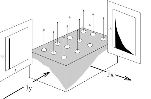
FIG. 1.: Illustrating the Hall response $j_{x}(t)=j_{o}\Theta_{H}(t)$ to an input current pulse $j_{y}(t)=j_{o}\delta(t)$.

Recent experimental advances make it possible to directly probe this Hall decay rate using optical transmission experiments. Such measurements by Kaplan et al[11] show that the frequency dependent Hall angle can be fit to a single Lorentzian form:

$$\theta_{H}(\omega)=\left[{\omega_{c}\over\Gamma_{H}-i\omega}\right]\;,$$ (10)

where $\Gamma_{H}$ is smaller than the transport relaxation rate. Measurements on $YBCO$ films at 100K indicate that $\Gamma_{H}\sim{1\over 4}\Gamma_{tr}$ at this temperature. At present, no detailed measurements of the temperature dependence of $\Gamma_{H}$ are available.

In this connection however, there is an important optical sum rule [12]

$$2\int_{0}^{\infty}{d\omega\over\pi}\theta_{H}(\omega)=\omega_{c}\;.$$ (11)

This is the transverse counterpart of the forward or “f-sum” rule. The transverse, or “t-sum rule” is exact, if all frequencies are included. For a single, split off-band, there is an effective sum rule with a cyclotron frequency

$$\omega_{c}=2eH{\sum{\rm det}(\underline{\rm m}_{p}^{-1})n_{p}\over\sum{\rm Tr}(\underline{\rm m}_{p}^{-1})n_{p}}\;,$$ (12)

which is determined by a sum over the entire band. This quantity is expected to be almost temperature independent. Since $\theta_{H}^{dc}\propto 1/T^{2}$, the width of the hall spectral function $\theta_{H}(\omega)$ must grow quadratically with temperature to preserve the sum rule. Measurements reported at this meeting[13] seem to provide some of the first direct support for this conclusion. It should be clear from this discussion, that the two-relaxation time interpretation of the cuprate transport can be made purely on the basis of the sum rule, and experimental observation.

Anderson’s interpretation of the Hall mobility in terms of two relaxation times nevertheless poses a serious paradox for the microscopic physics. The problem is, that in a conventional metal there is no microscopic distinction between a “Hall” and an “electric” current. Electrons respond to the total Lorentz electric field

$$\vec{\cal E}=\vec{E}+\vec{v}\times\vec{H}\;,$$ (13)

where $\vec{v}$ is their group velocity. Electric and magnetic fields always enter the transport equations in this combination, so that electrons on the Fermi surface can not tell external electric and internal Lorentz forces apart. Anderson has suggested that one way to produce two such autonomous scattering rates is to develop spin-charge decoupling. In his picture, the $T^{2}$ scattering rate is associated with spin excitations, or “spinons”, whilst the linear relaxation rate is associated with charge excitations, or “holon”. Anderson suggests that the motion of spinons produces a charge back-flow which is responsible for the Hall current. What is lacking is an explanation of why this charge back-flow only carries a Hall current. To pursue the idea of two transport relaxation times we need to find a symmetry reason for this selectivity.

Before taking this path it is instructive to consider the alternatives. Two classes of proposal have been made:

• Strong momentum-dependent scattering.[14, 15, 16]

• Skew scattering.[17]

The first scenario[14, 15, 16] envisions two distinct regions of the Fermi surface: a “hot spot” where the scattering rate is a linear function of temperature, $\Gamma_{{\rm hot}}\propto T$, and a second “cold” region of the Fermi surface with a weaker temperature dependence of the transport relaxation rate $\Gamma_{{\rm cold}}$. This theory presumes that the “hot spot” dominates the electrical conductivity, whereas the cold region, with a higher Fermi surface curvature, sets the Hall conductivity, so that

$$\sigma_{xx} \propto {1\over\Gamma_{{\rm hot}}}\;,$$ (14)

$$\sigma_{xy} \propto {H\over(\Gamma_{{\rm cold}})^{2}}\;.$$ (15)

In this interpretation, the quadratic temperature dependence of the Hall relaxation rate is not fundamental, but appears as a consequence of a cancelation between relaxation rates at different parts of the Fermi surface:

$$\Gamma_{H}\propto{\Gamma_{{\rm cold}}^{2}\over\Gamma_{{\rm hot}}}\;,\qquad(\hbox{\rm``hot \ spot \ scenario''}).$$ (16)

If $\Gamma_{{\rm cold}}\propto T^{1.5}$, then $\Gamma_{H}\propto T^{2}$.

The “skew scattering” interpretation of the anomalous Hall angle, presumes the presence of chiral current fluctuations which, through their coupling to the electrons cause a field-dependent “skew scattering” component to develop in the inelastic scattering. This component is required to have a singular dependence on temperature of the following form

$$\Gamma_{\rm skew}\propto{H\over T}\;.$$ (17)

The skew-scattering renormalizes the effective cyclotron frequency without changing the current relaxation rates, changing $\omega_{c}\rightarrow\omega_{c}^{*}=\omega_{c}+\Gamma_{\rm skew}$, so that for an almost compensated band $\omega_{c}^{*}\sim\Gamma_{\rm skew}$ giving

$$\Gamma_{H}(T)\propto{\Gamma_{\rm tr}\over\Gamma_{\rm skew}}\;,\qquad({\rm skew\ scattering})$$ (18)

is a quadratic function of temperature.

These alternate scenarios face a serious common difficulty. Each case requires the presence of a fortuitous cancelation of two independent scattering processes. The temperature dependences $\Gamma_{\rm hot}\propto T^{1.5}$ and $\Gamma_{\rm skew}\propto 1/T$ are actually more complicated than the simple quadratic relaxation rate they are supposed to give rise to. Furthermore in these theories, if the linear transport relaxation rate is substantially modified by the addition of impurities or changes in the hole concentration, then the quadratic temperature dependence of $\Gamma_{H}$ is lost. This is not what is seen: changes in impurity concentration or oxygen doping which eliminate the linear temperature dependence of the resistivity do not change the the quadratic temperature dependence of $\Gamma_{H}$. These features all tend to suggest that $\Gamma_{H}$ is a truly autonomous scattering rate, not a fortuitous cancelation of other scattering processes.

So to conclude this section, rather general considerations of an experimental and theoretical nature appear to force us to return to Anderson’s original conjecture and to ask what general constraints it places on the microscopic physics. This is the subject of the remainder of this paper.

III Symmetries of the Fermi surface

What type of scattering event can lead to different Hall and electric relaxation rates? Fundamentally, electrical and Hall currents differ in the number of photons absorbed. In linear response theory, electric current involves the absorption of a single photon with a finite frequency. The Hall current is generated by a two-photon absorption process: the first photon excites an electron-hole pair about the Fermi surface, the second transfers momentum, causing the electron and hole in the pair to precess around the Fermi surface. The diagrammatic expression of the electric and Hall conductivities involves the bubble and triangle diagrams shown in Fig. 2

.

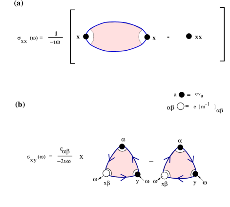
FIG. 2.: (a) “Bubble diagram entering conductivity, (b) “Triangle diagrams” entering into the Hall conductivity. Open circle denotes the effective mass tensor which appears when the derivative of the velocity operator with respect to the external momentum is taken, to extract the magnetic field dependence (See Appendix A). Filled circle denotes the velocity operator.

Heuristically

$$\sigma_{xx}(\omega) \sim {{\rm bubble\ diagram}(\omega)\over-i\omega},$$ (19)

$$\sigma_{xy}(\omega) \sim {1\over\omega}\bigl{[}{\rm triangle\ diagram}(\omega)\bigr{]}.$$ (20)

Each external leg of the diagram carries the same momentum, and thus the relaxation times which enter multiplicatively into the Hall conductivity must be derived from the same point in momentum space. How then can a two-photon process involve the product of two qualitatively different relaxation time-scales?

The shrewd diagrammatician will recognize that, in general, we have to include vertex corrections and that if these are important a simple relaxation time discussion of the problem may not be valid. Recall however, that the qualitative simplicity of the experiment suggests that the underlying physics does have some kind of simple relaxation time interpretation, albeit not the one we are familiar with. In conventional metals the effect of vertex corrections is to replace the electron inelastic scattering rate by the appropriate transport relaxation rate

$$\Gamma(\omega,\vec{p})\ \ \mathrel{\mathop{\mathrel{\mkern-8.0mu}\relbar\mathrel{\mkern-8.0mu}\relbar\mathrel{\mkern-8.0mu}\relbar\mathrel{\mkern-8.0mu}\relbar\mathrel{\mkern-8.0mu}\relbar\mathrel{\mkern-8.0mu}\relbar\mathrel{\mkern-8.0mu}\relbar\mathrel{\mkern-8.0mu}\relbar\mathrel{\mkern-8.0mu}\longrightarrow}^{\rm vertex\ eff.}}\ \Gamma_{\rm tr}(\omega,\vec{p})\;,\qquad(\rm simple\ metal)\;.$$ (21)

Experiments motivate us to seek an explanation where the effect of the vertices is to produce two relaxation times on the external legs

$$\Gamma(\omega,\vec{p})\ \ \mathrel{\mathop{\mathrel{\mkern-8.0mu}\relbar\mathrel{\mkern-8.0mu}\relbar\mathrel{\mkern-8.0mu}\relbar\mathrel{\mkern-8.0mu}\relbar\mathrel{\mkern-8.0mu}\relbar\mathrel{\mkern-8.0mu}\relbar\mathrel{\mkern-8.0mu}\relbar\mathrel{\mkern-8.0mu}\relbar\mathrel{\mkern-8.0mu}\longrightarrow}^{\rm vertex\ eff.}}\ \left\{\begin{array}[]{rl}\displaystyle\Gamma_{\rm tr}&\displaystyle(\omega,\vec{p})\;,\cr\displaystyle\Gamma_{\rm H}&\displaystyle(\omega,\vec{p})\;.\end{array}\right.$$ (24)

We seek an explanation where the one photon absorption process involves the fast relaxation rate $\Gamma_{\rm tr}$, but the two-photon absorption process, involves a product of both relaxation times.

There is a vital distinction between the electrical and Hall current. Magnetic fields couple to the the momentum dependent part of the current operator, and it is this component that gives rise to a Hall response. Operationally, the momentum derivative which enters in the Hall conductivity acts on the vertices of the Hall conductivity, extracting the momentum dependent part of the current operator. If we are to understand the two-relaxation time interpretation then we must understand what feature of the scattering processes can force the momentum dependent part of the current operator to develop a different relaxation rate.

We now examine the symmetries that delineate Hall and electric current. There are three fundamental symmetry operations that describe the excitations around a Fermi surface: time-reversal ($T$), inversion ($P$) and charge conjugation symmetry ($C$). Consider a Fermi surface where the kinetic energy is defined by the Hamiltonian

$$H_{o}=\sum_{\rm p\sigma}\epsilon_{\rm\vec{p}}\psi{{}^{{\dagger}}}_{\rm\vec{p}\sigma}\psi_{\rm\vec{p}\sigma}\;.$$ (25)

To make our discussion precise, we suppose that throughout any calculation of current response functions, we may approximate the Fermi surface by a polyhedron where the center of each face is the Fermi wave-vector $\vec{p}_{F}$. At the end of the calculation, the number of sides of the polyhedron is to be taken to infinity. Consider an electron state with momentum $\vec{p}=\vec{p}_{F}+\delta\vec{p}$, near a Fermi surface. This state is degenerate with a hole state formed by annihilating an electron at momentum $\vec{p}^{*}=\vec{p}_{F}-\delta\vec{p}^{*}$ ($\epsilon_{\rm\vec{p}}=-\epsilon_{\rm\vec{p}^{*}}$) . The operation that links the two states is that of charge conjugation. It is also degenerate with the up and down electron states at momentum $-\vec{p}$ that we obtain by space or time reversal operations. We define the set of three symmetry operations as follows :

$$C{{}^{{\dagger}}}\psi_{\vec{p}\sigma}C = \sigma\psi{{}^{{\dagger}}}_{\vec{p}^{*}\ -\sigma},$$ (26)

$$P{{}^{{\dagger}}}\psi_{\vec{p}\sigma}P = \psi_{-\vec{p}\sigma},$$ (27)

$$T{{}^{{\dagger}}}\psi_{\vec{p}\sigma}T = \sigma\psi_{-\vec{p}\ -\sigma}.$$ (28)

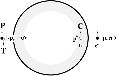
FIG. 3.: Illustrating the action of operators $C$, $P$ and $T$ on the electron state $|\vec{p},\sigma\rangle$.

Charge conjugation changes the charge of the quasiparticle, but does not alter it’s velocity. Parity and time reversal change the velocity of the quasiparticle, (Fig. 3) without changing its charge, as follows:

$$\hat{C}:\qquad{\rm e} \longrightarrow -{\rm e},$$ (29)

$$\hat{P},\ \hat{T}:\qquad{\vec{v}} \longrightarrow -{\vec{v}}.$$ (30)

Time-reversal also flips the spin of the quasiparticle. These operators span a manifold of eight degenerate electron and hole states on opposite sides of the Fermi surface. Provided the relevant physics involves electron states near enough to the Fermi surface, we expect these symmetries to be preserved by interactions. This is the case, for instance, in the one-dimensional Luttinger liquid. These symmetries are also preserved in the presence of a magnetic field, where

$$H_{o}[\vec{A}]=\sum_{\rm p\sigma}\epsilon_{\rm\vec{p}-e\vec{A}}\psi{{}^{{\dagger}}}_{\rm\vec{p}\sigma}\psi_{\rm\vec{p}\sigma}\;.$$ (31)

Using the properties $\epsilon_{\rm\vec{p}}=\epsilon_{-\rm\vec{p}}=-\epsilon_{-\rm\vec{p}^{*}}$, the Hamiltonian transforms as follows

$${\cal O}{{}^{{\dagger}}}H[\vec{A}]{\cal O}=H[-\vec{A}],\qquad({\cal O}=C,\ P,\ T),$$ (32)

so that these transformations are equivalent to changing the external field $\vec{A}\longrightarrow\vec{A}^{*}=-\vec{A}$, or more correctly

$$\vec{A}^{*}(x,t)=\left\{\begin{array}[]{rcl}\displaystyle-\vec{A}(x,t),&&(C)\cr-\vec{A}(-x,t),&&(P)\cr-\vec{A}(x,-t).&&(T)\end{array}\right.$$ (36)

Suppose $|\Psi_{o}\rangle$ is a current-free state of the normal metal. If an external field is applied to this state, the current carrying state which develops is

$$|E,H\rangle={\cal T}e^{i\int(\vec{A}\cdot\vec{j})d^{3}xdt}|\Psi_{o}\rangle,$$ (37)

where ${\cal T}$ denotes the time-ordered product, $\vec{E}$ and $\vec{H}$ are the electric and magnetic fields. Now consider the transformed state

$$|E^{*},H^{*}\rangle={\cal O}|E,H\rangle.$$ (38)

Since $|\Psi_{o}\rangle$ carries no current, we expect it to be symmetric under $P$, $C$ and $T$, ${\cal O}|\Psi_{o}\rangle=|\Psi_{o}\rangle$. Thus

$$|E^{*},H^{*}\rangle={\cal T}e^{i\int(\vec{A}^{*}\cdot\vec{j})d^{3}xdt}|\Psi_{o}\rangle\;,$$ (39)

corresponds to the state which would evolve in response to the transformed electric and magnetic fields, $\vec{E}^{*}=-\partial\vec{A}^{*}/\partial t$ and $\vec{H}^{*}=\vec{\nabla}\times\vec{A}^{*}$. The parities of these fields under $C$, $P$ and $T$ are then

	$\quad A\quad$	$\quad E\quad$	$\quad H\quad$
C	-	-	-
P	-	-	+
T	-	+	-

.

We can work out the parities of the electric $\vec{\cal J}_{E}$ and Hall current $\vec{\cal J}_{H}$ operators under these various transformations by comparing their expectation values in the two states $|E,H\rangle$ and $|E^{*},H^{*}\rangle$,

$${j}^{*}_{E,H} = \langle E^{*},H^{*}|{\cal J}_{E,H}|E^{*},H^{*}\rangle\;,$$ (40)

$$j_{E,H} = \langle E,H|{\cal J}_{E,H}|E,H\rangle.$$ (41)

To find the parities, we may apply the transformations $(E,\ H)\rightarrow(E^{*},\ H^{*})$ to the classical equations of motion,

$$\vec{j}_{E} \sim {ne^{2}\over m}\int\vec{E}dt,$$ (42)

$$\vec{j}_{H} \sim {e\over m}\int\vec{j}_{E}\times\vec{H}dt.$$ (43)

It follows that electric current transforms in the same way as the vector potential $\vec{\cal J}_{E}\sim\vec{A}$, whereas Hall current transforms in the same way as the Poynting vector $\vec{E}\times\vec{H}$. The parities of these two currents are thus given by the following table

	$\quad{\cal J}_{E}\sim\vec{A}\quad$	$\quad{\cal J}_{H}\sim\vec{E}\times\vec{H}\quad$
C	-	+
P	-	-
T	-	-

.

Charge conjugation parity uniquely discriminates between Hall and electric currents.

We may confirm the results of this heuristic discussion by directly applying the transformation operators to the total current operator. Under $\hat{P}$ and $\hat{T}$, the entire current operator transforms in the same way, and it is only under $\hat{C}$ that it divides up into two components of opposite parity.

Using this information we can construct the Hall and electric current operators as follows. Suppose the wave-function for a metal in an electro-magnetic field is $|\vec{E},\vec{H}\rangle$. We may construct the state in which the electric and magnetic fields are reversed by applying the charge conjugation operator

$$|- \vec{E},\ -\vec{H}\rangle =\hat{C}|\vec{E},\vec{H}\rangle.$$ (44)

The current in this state is given by

$$\langle-\vec{E},\ -\vec{H}|\vec{\cal J}|-\vec{E},\ -\vec{H}\rangle$$ (45)

$$=\langle\vec{E},\ \vec{H}|C{{}^{{\dagger}}}\vec{\cal J}C|\vec{E},\ \vec{H}\rangle..$$ (46)

In the original state $|E,H\rangle$ state, the total current is given by a sum of electric and Hall currents

$$\langle\vec{E},\ \vec{H}|\vec{\cal J}|\vec{E},\ \vec{H}\rangle=\vec{j}_{E}+\vec{j}_{H}.$$ (47)

In the state with reversed fields, the electric current reverses, but the Hall current does not, i.e.

$$\langle\vec{E},\ \vec{H}|C{{}^{{\dagger}}}\vec{\cal J}C|\vec{E},\ \vec{H}\rangle=-\vec{j}_{E}+\vec{j}_{H}.$$ (48)

It follows that the uniform electric and Hall current operators may be defined as follows

$$\vec{\cal J}_{\textstyle\left\{{E\above 0.0ptH}\right\}} = {1\over 2}[\vec{\cal J}\mp C{{}^{{\dagger}}}\vec{\cal J}C].$$ (49)

When we explicitly evaluate these operators near the Fermi surface, we find that

$$\vec{\cal J}_{E} = e\sum_{\rm\vec{p}\sigma}\vec{v}_{F}\psi{{}^{{\dagger}}}_{\rm\vec{p}\ \sigma}\psi_{\rm\vec{p}\ \sigma},\qquad(C=-1)$$ (50)

$$\vec{\cal J}_{H} = e\sum_{\rm\vec{p}\sigma}\psi{{}^{{\dagger}}}_{\rm\vec{p}\ \sigma}\underline{\rm m}^{-1}{(\delta\rm\vec{p}-e\vec{A})}\psi_{\rm\vec{p}\sigma},\qquad(C=+1)$$ (51)

where we have expanded the electron velocity in terms of the effective mass tensor near the Fermi surface. The Hall current is zero when the Fermi surface is flat.

Notice how the electric and Hall current depend on changes in the electron occupation that are respectively even and odd about the Fermi surface. Magnetic photons introduce a small shift in the momentum $\delta q$ and this gives rise to Hall current proportional to $\delta q$. If Hall and electric currents relax at qualitatively different rates then there must be scattering processes which selectively relax these two different types of quasiparticle distribution. In other-words, the scattering, and hence the microscopic self-energies of the electrons must depend on charge conjugation symmetry. Schematically, if $\underline{\Sigma}$ is the electron self energy, then we require

$$\underline{\Sigma}={\Sigma}_{1}+{\Sigma}_{2}\tilde{C},$$ (52)

where $\tilde{C}$ is one of $C$, $CP$, $CT$ or $CPT$.

There are two points to discuss about this conclusion. First, we may reject the possibilities $\tilde{C}=CP$ or $\tilde{C}=CT$, because under these transformations the electric current is an even-parity operator and the Hall current is an odd-parity operator. We shall shortly see that even-parity operators are always “short-circuited” by the quasiparticles with the slowest relaxation rate, whereas odd-parity operators are governed by quasiparticles with the fastest relaxation rate. If $\tilde{C}=CT$ or $CP$, it would mean Hall currents relax more rapidly than electric currents. This is a situation that actually occurs in the vicinity of a superconducting transition, where the presence of a pairing field introduces scattering that is sensitive to $\tilde{C}=CP$.[19] In our case however, optical Hall measurements[11] already rule this possibility out. The operators $C$ and $CPT$ differ only in a spin-flip and for spin-less properties, they are essentially indistinguishable. We shall chose $\tilde{C}=C$, but our arguments are readily modified to accommodate the alternative choice $\tilde{C}=CPT$.

Second, we must be careful about the literal interpretation of Eq. 52. The charge conjugation operator does not commute with charge, so a term of the type we are proposing can not exist in an environment of unbroken symmetry. This faces us with a dilemma, for we know that on a macroscopic scale, the normal state of the cuprates has no broken symmetry. Our symmetry analysis forces us to conclude that if the Hall and electric currents have different decay rates, then the electrons must perceive their local environment as having developed a broken symmetry. We are thus forced to conclude that there must be some kind of low-energy, charge carrying excitation whose fluctuations create a local environment which is symmetry-broken on a time-scale $\tau\gtrsim\tau_{tr}$. From this point-of-view, (52) should be regarded as a mean-field assumption that the charge carrying fluctuations produced by this environment are sufficiently slow, that the vertex corrections can be captured by an anomalous self-energy. We shall return to this point in the final section.

If indeed scattering is sensitive to the charge conjugation parity, then we might expect other transport currents to reflect these two transport relaxation times. Neutral currents, such as the thermal or thermo-electric current are also even under the charge conjugation operator, thus we expect that their relaxation will be governed by the same $T^{2}$ relaxation rate as the Hall current. Circumstantial support for this idea is obtained from the thermopower of optimally doped compounds.

Thermal and electric transport is normally described in terms of four fundamental transport tensors[20]

$$\begin{array}[]{cc}\vec{j}_{e}&=\underline{\sigma}\vec{E}+\underline{\beta}\vec{\nabla}T\;,\\ \vec{j}_{t}&=\underline{\gamma}\vec{E}+\underline{\zeta}\vec{\nabla}T\;.\end{array}$$ (53)

These tensors are directly linked to microscopic charge and thermal current fluctuations via Kubo formulae. Table I compares the leading temperature dependences of the various transport tensors measured in the optimally doped cuprates with a series of calculations we now describe. The thermo-electric conductivity $\underline{\beta}$, determined from the conductivity and Seebeck coefficients, $\underline{S}$, $\underline{\beta}=-\underline{\sigma}\underline{S}$ has a particularly revealing temperature dependence. In a naïve relaxation-time treatment, the temperature dependence of $\beta$ is directly related to the relevant quasiparticle relaxation rate $\tau_{TE}^{-1}$ according to[21]

$$\beta=-\left(\pi^{2}k_{B}\over 3e\right)\left(k_{B}T\over\epsilon_{F}\right){ne^{2}\over m}\tau_{TE}\;,$$ (54)

where $\epsilon_{F}$ is the Fermi energy. Combining this with the electrical conductivity, $\sigma={ne^{2}\over m}\tau_{tr}$, the dimension-less thermopower is then

$$\tilde{S}={eS\over k_{B}}=\left({\tau_{TE}\over\tau_{tr}}\right)\left({\pi^{2}\over 3}\right)\left({k_{B}T\over\epsilon_{F}}\right)\;.$$ (55)

In optimally doped compounds[22], the thermopower contains an unusual constant part, $\tilde{S}\approx\tilde{S}_{o}-bT$ where $\tilde{S}_{o}\sim 0.1$, which indicates that

$$\tau^{-1}_{TE}={T^{2}/W_{th}}\;,$$ (56)

is a factor $T/\eta W_{th}$ smaller than the transport relaxation rate, where $W_{th}=(3\tilde{S}_{o}/\pi^{2}\eta)\epsilon_{F}\sim{\epsilon_{F}/10}$. The comparable size and temperature dependence of $\tau^{-1}_{TE}$ and $\tau^{-1}_{H}$ suggest that the same type of quasiparticle carries both the Hall current and the thermo-current.

IV Charge Conjugation Eigenstates and the Derivation of the Transport Equation

Having argued the case for a scattering mechanism which is sensitive to charge-conjugation parity, we now establish the effect on the transport properties. We need to express currents in terms of charge-conjugation eigenstates rather than the charge eigenstates, electrons (and holes) that we are familiar with. This amounts to a change of basis. While the self-energy of the carriers will now be diagonal in this new basis, external applied fields will, in general, be able to inter-convert the two charge conjugation eigenstates.

The eigenstates of the charge conjugation operator defined in Eq. 28 may be written

$$\begin{array}[]{rcl}\displaystyle a_{{\rm\vec{p}}\sigma}&=&\displaystyle{{1\over\sqrt{2}}}[\psi_{{\rm\vec{p}}\sigma}+\sigma\psi{{}^{{\dagger}}}_{{\rm\vec{p}}^{*}-\sigma}],\qquad(C=+1)\\ \displaystyle b_{{\rm\vec{p}}\sigma}&=&\displaystyle{{1\over\mbox{i}\sqrt{2}}}[\psi_{{\rm\vec{p}}\sigma}-\sigma\psi{{}^{{\dagger}}}_{{\rm\vec{p}}^{*}-\sigma}].\qquad(C=-1)\end{array}$$ (57)

Fermions which are eigenstates of the charge conjugation operator were first introduced by Majorana over sixty years ago and, for this reason, are called, “Majorana” fermions.[23] When we construct a Majorana representation of the Fermi surface we are, in essence, folding the quasiparticle states inside the Fermi surface to the outside. The momenta of all Majorana fermions are restricted to the outside of the Fermi surface, for particles inside the Fermi surface are the anti-particles of those outside. Our central hypothesis is that quasiparticle-states of opposite charge conjugation parity have different relaxation rates.

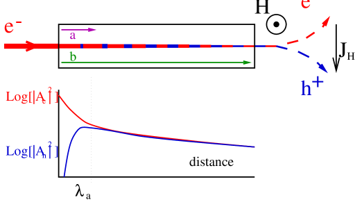
FIG. 4.: A simple picture of transport where relaxation processes are sensitive to charge conjugation parity. An electron current converts into an equal mixture of $a$ and $b$ charge conjugation eigenstates. One parity decays rapidly leaving a neutral current with equal numbers of electrons and holes moving together. In a magnetic field this neutral current can still induce a Hall voltage.

To illustrate how this leads to distinct relaxation rates controlling the Hall and electric currents, consider the thought experiment illustrated in Fig. 4. Imagine a flux of electrons injected into a block of cuprate metal. Inside the metal we must consider these electrons to be a linear combination of $a$ and $b$ states

$$\psi^{\dagger}_{{\rm\vec{p}}\sigma}\longrightarrow a^{\dagger}_{{\rm\vec{p}}\sigma}+ib^{\dagger}_{{\rm\vec{p}}\sigma}\;.$$ (58)

As the $a$ and $b$ quasiparticles propagate through the metal one species, say $a$, rapidly decays and becomes incoherent. At distances greater than the mean free path of the $a$ quasiparticles only $b$ particles remain. The residual current is neutral, with equal numbers of electrons and holes moving at the same velocity. Charge transport is thus controlled by the short mean free path. However, should the $b$ particle flux move through a region of finite magnetic field, the Lorentz force will deflect the electron and hole components in opposing tangential directions. Since this neutral current can generate a finite Hall current, the Hall response is controlled by the longer mean free path. From this simple thought experiment we may make the following general observations which will apply to this phenomenology

• the physics is insensitive to which $C$ eigenstate decays faster,

• to cleanly disentangle the separate lifetimes requires that $\Gamma_{f}\gg\Gamma_{s}$,

• were we to repeat the thought experiment choosing instead eigenstates of $\tilde{C}=CP$ or $CT$ — i.e. linear combinations of electrons and holes moving with opposite velocities — then in this case the long-lived quasiparticle carries electric current. However, application of a magnetic now deflects the electron and hole components in the same direction, so there is no Hall response. So in this case, Hall currents decay quickly and electric currents decay slowly. This is the situation near a superconducting phase transition, where the long-lived quasiparticles at the Fermi surface are eigenstates of $CP$.[19]

We now develop the transport theory which follows from our phenomenological assumption. We will not discuss spin transport, restricting our attention to a simplified, spin-less electron fluid . One may use diagrammatic perturbation theory to derive the conductivities and this is done in Appendix B for completeness. However, since high order transport properties (such as the magneto-conductance) require the careful analysis of rather a large number of diagrams, we also develop a Boltzmann transport equation. In the limit of well defined quasi-particles near the Fermi surface, the results are equivalent. The derivation of the Boltzmann equation is again somewhat technical and may be found in Appendix C. There we derive the following matrix generalization of the Boltzmann equation

$$\underline{\dot{\rm f}}+{\textstyle{1\over 2}}\left\{\underline{\vec{\cal V}}_{{\rm\vec{p}}},\vec{\nabla}_{\rm R}\underline{\rm f}\right\}_{+}+{\textstyle{e\over 2}}\left\{(\vec{\rm E}+\underline{\vec{\cal V}}_{{\rm\vec{p}}}\times\vec{\rm B})\underline{\tau}_{2},\vec{\nabla}_{\rm p}\underline{\rm f}\right\}_{+}={\rm I}[\underline{g}]\;,$$ (59)

where

$$\underline{\vec{\cal V}}_{\vec{p}}={1\over 2}\left(\vec{v}_{\vec{p}}+\vec{v}_{\vec{p}*}\right)\underline{1}+{1\over 2}\left(\vec{v}_{\vec{p}}-\vec{v}_{\vec{p}*}\right)\underline{\tau}_{2}\;,$$ (60)

and

$$\underline{f}(t,\vec{R},\vec{p}) = \left(\begin{array}[]{cc}\langle a^{\dagger}_{\vec{p}}a_{\vec{p}}\rangle&\langle b^{\dagger}_{\vec{p}}a_{\vec{p}}\rangle\\ \langle a^{\dagger}_{\vec{p}}b_{\vec{p}}\rangle&\langle b^{\dagger}_{\vec{p}}b_{\vec{p}}\rangle\end{array}\right)_{\vec{R},t}\;$$ (63)

is the quasiparticle density matrix. This matrix measures the local density of quasiparticles at the course-grained point $\vec{R}$ and its off-diagonal elements allow for the quantum superposition of $a$ and $b$ particles.

We see that the left hand side of the transport equation is similar to a conventional Boltzmann equation: there are driving terms due to gradients in the distribution function and due to electro-magnetic fields. The new features are the anti-commutators, which come from making a gradient expansion with matrices rather than single functions, and the presence of the second Pauli matrix $\underline{\tau}_{2}$. This is a reflection of the fact that the EM field couples to charge and, since $a$ and $b$ do not have well defined charge, they can be inter-converted by the applied field.

The right-hand side of the transport equation contains the essence of our phenomenology: the collision integral. It is a functional of the departure from the equilibrium distribution $\underline{g}=\underline{\rm f}-\underline{\rm f}^{(0)}$. The simplicity of the experiments forces us to the hypothesis that the return to equilibrium is governed by two independent relaxation times—one for each of the charge conjugation eigenstates. This is represented by the collision integral

$${\rm I}[\underline{g}]=-{1\over 2}\left\{\underline{\Gamma},\underline{g}\right\}_{+}=-{1\over 2}\left\{\left(\begin{array}[]{cc}\Gamma_{f}&0\\ 0&\Gamma_{s}\end{array}\right),\underline{g}\right\}_{+}\;.$$ (64)

Putting $\Gamma_{f}=\Gamma_{s}$ one recovers the usual relaxation time approximation of text book treatments.

Our transport equations are completely general for arbitrary Fermi surface and anisotropic scattering rates but, as we have shown, including these features will not account for the products in relaxation rates appearing experimentally in magneto-transport. We therefore make the simplifying assumption that we have a cylindrical Fermi surface and that $\Gamma_{f}$ and $\Gamma_{s}$ are momentum independent.

Setting up the transport equation under these conditions we note that, near the Fermi surface, we have $\delta p^{*}=\delta p+O(\delta p^{2}/p_{F})$ where the small correction does not enter into the leading order (in $T/E_{F}$) transport coefficients. We may therefore write

$$\underline{\vec{\cal V}}_{\vec{p}}=\vec{v}_{F}\underline{1}+\left({\delta\vec{p}\over m}\right)\underline{\tau}_{2}\;,$$ (65)

where $\vec{v}_{F}$ and $\delta\vec{p}\;(\geq 0)$ are normal to the Fermi surface. For the in-plane transport properties we discuss here, $\vec{E}$ and $\vec{\nabla}T$ lie in the basal plane and the magnetic field is always perpendicular to the cuprate layers.

In the absence of applied fields, the distribution of quasiparticles is given by a diagonal matrix since, by construction, the Hamiltonian is diagonal in the basis of our charge conjugation eigenstates:

$$\underline{\rm f}^{0}_{\vec{p}}={1\over 2}\left[n_{F}(\epsilon_{p})+n_{F}(-\epsilon_{p^{*}})\right]\underline{1}\;.$$ (66)

The derivative, ${\vec{\nabla}}_{\vec{p}}\underline{\rm f}^{0}_{\vec{p}}=n_{F}^{\prime}\underline{\vec{\cal V}}_{\vec{p}}$, is not purely diagonal. Here $n_{F}^{\prime}$ is energy derivative of the Fermi function $\partial_{\epsilon}n_{F}(\epsilon_{\vec{p}})$.

By expressing the deviation from the equilibrium distribution in the Pauli matrix basis $\underline{g}_{\vec{p}}=g_{0}({\vec{p}})\underline{1}+{\vec{g}}(\vec{p})\cdot\underline{\vec{\tau}}$ and substituting into the Boltzmann equation, we find that the component $g_{1}$ decouples. The remaining components satisfy

$$\left(\underline{a}+\underline{b}\right)\left(\begin{array}[]{c}g_{0}(\vec{p})\\ g_{2}(\vec{p})\\ g_{3}({\vec{p}})\end{array}\right)=c\;,$$ (67)

where, with $\Gamma_{\pm}=(\Gamma_{f}\pm\Gamma_{s})/2$, we have

$$\underline{a}=\left(\begin{array}[]{ccc}\Gamma_{+}&0&\Gamma_{-}\\ 0&\Gamma_{+}&0\\ \Gamma_{-}&0&\Gamma_{+}\end{array}\right)\quad\;,\quad\underline{b}=\left(\begin{array}[]{ccc}h_{\vec{p}}&w_{\vec{p}}&0\\ w_{\vec{p}}&h_{\vec{p}}&0\\ 0&0&h_{\vec{p}}\end{array}\right)\;,$$ (68)

$$c=-n_{F}^{\prime}\left(\begin{array}[]{c}e{\vec{E}}\cdot{\delta\vec{p}}/m-v_{F}^{2}\hat{p}\cdot{\vec{\nabla}T}/T\\ ev_{F}{\vec{E}}\cdot\hat{p}-(v_{F}/m)\delta{\vec{p}}\cdot{\vec{\nabla}T}/T\\ 0\end{array}\right)\;,$$ (69)

with

$$h_{\vec{p}} = v_{F}\hat{p}\cdot{\vec{\nabla}}T\partial_{T}+({e/m})\delta{\vec{p}}\times{\vec{H}}\cdot{\vec{\nabla}}_{\vec{p}}\;,$$ (70)

$$w_{\vec{p}} = (\delta\vec{p}/m)\cdot{\vec{\nabla}T}\partial_{T}+e\left({\vec{E}}+v_{F}\hat{p}\times{\vec{H}}\right)\cdot{\vec{\nabla}}_{\vec{p}}\;.$$ (71)

We solve these equations using the Zener-Jones method [8], solving order by order in the fields. We may write the solutions schematically as

$$g^{(n)}=\left(-\underline{a}^{-1}\underline{b}\right)g^{(n-1)}\quad,\quad g^{(1)}=\underline{a}^{-1}c\;.$$ (72)

The first order solution is

$$g_{2}^{(1)} = -{n_{F}^{\prime}\over\Gamma_{+}}\left(ev_{F}{\vec{E}}\cdot\hat{p}-{v_{F}\over mT}\delta{\vec{p}}\cdot{\vec{\nabla}T}\right)\;,$$ (73)

$$\left[\begin{array}[]{c}g_{0}^{(1)}\\ g_{3}^{(1)}\end{array}\right] = -{n_{F}^{\prime}\over\Gamma_{f}\Gamma_{s}}\left[\begin{array}[]{c}\Gamma_{+}\\ \Gamma_{-}\end{array}\right]\left({e{\vec{E}}\cdot\delta{\vec{p}}\over m}-{v_{F}^{2}\over T}\hat{p}\cdot{\vec{\nabla}T}\right)\;.$$ (78)

This is sufficient to compute the lowest order transport coefficients. Off-diagonal conductivities come from the second-order solution. The magnetic field dependent part of $g^{(2)}$ is then

$$g_{2}^{(2)}={en_{F}^{\prime}\over m}\left[{ev_{F}\hat{p}\times{\vec{H}}\cdot{\vec{E}}\over\Gamma_{f}\Gamma_{s}}-{v_{F}\delta p^{2}{\hat{p}}\times\vec{H}\cdot{\vec{\nabla}T}\over\Gamma_{+}^{2}mT}\right],$$ (79)

$$\left[\!\!\begin{array}[]{c}g_{0}^{(2)}\\ g_{3}^{(2)}\end{array}\!\!\right]\!\!\!=\!{-en_{F}^{\prime}\over m\Gamma_{f}\Gamma_{s}}\!\!\left[\begin{array}[]{ccc}{{\Gamma_{+}^{2}-\Gamma_{-}^{2}}\over\Gamma_{f}\Gamma_{s}}&-1&0\\ {2\Gamma_{+}\Gamma_{-}\over\Gamma_{f}\Gamma_{s}}&0&{\Gamma_{-}\over\Gamma_{+}}\end{array}\right]\!\!\!\left[\begin{array}[]{c}\displaystyle{\rm e\delta{\vec{p}}\times{\vec{H}}\cdot{\vec{E}}\over m}\\ \displaystyle{\rm v_{F}^{2}\delta\vec{p}\times\vec{H}\cdot\vec{\nabla}T\over T}\\ \displaystyle{\rm v_{F}\delta p{\vec{p}}\times\vec{H}\cdot\vec{\nabla}T\over mT}\end{array}\right].$$ (80)

Finally we require the third order solution to obtain the magneto-conductivity. Assuming no temperature gradient the leading term in $T/E_{F}$ will come from

$$g^{(3)}_{2}={-e^{3}n_{F}^{\prime}v_{F}\over m^{2}\Gamma_{+}}{\Gamma_{+}^{2}+\Gamma_{-}^{2}\over(\Gamma_{f}\Gamma_{s})^{2}}(\hat{p}\times\vec{H})\cdot(\vec{E}\times\vec{H})\;.$$ (81)

Having solved the Boltzmann equation we determine the conductivities from the current response in applied fields. The electric and thermal currents may be written in terms of $\underline{g}$ as follows

$$\vec{j}_{e} = \sum_{\vec{p}>p_{F}}2ev_{F}\hat{p}g_{2}(\vec{p})+2{e\over m}\delta\vec{p}g_{0}(\vec{p})\;,$$ (82)

$$\vec{j}_{t} = \sum_{\vec{p}>p_{F}}2v_{F}^{2}\delta\vec{p}g_{0}(\vec{k})+2{v_{F}\delta p^{2}\over m}\hat{p}g_{2}(\vec{k})\;.$$ (83)

The conductivities can then be extracted and we summarize the results in the second column of Table I.

TABLE I.: Leading temperature dependences of transport coefficients compared with proposed decomposition into two Majorana relaxation times (${\cal L}_{0}$ is the Lorentz number $\pi^{2}k_{B}^{2}/3e^{2}$).

Cond-	Majorana	Leading T behavior
uctivity	Fluid	$\Gamma_{f}\gg\Gamma_{s}$
	$\times\left({m\over ne^{2}}\right)$	$(T\gg T^{2})$	Expt.	Ref.
$\sigma_{\rm xx}$	${\displaystyle 2\over\displaystyle\Gamma_{f}+\Gamma_{s}}$ $\biggl{(}$	$T^{-1}$	$T^{-1}$
$\sigma_{\rm xy}$	${\displaystyle\omega_{c}\over\displaystyle\Gamma_{f}\Gamma_{s}}$ $\biggl{(}$	$T^{-3}$	$T^{-3}$
$\Delta\sigma_{\rm xx}$	$-{\displaystyle\sigma_{xx}\over\displaystyle 2}\bigl{(}{\displaystyle{\omega_{c}^{2}\over\Gamma_{s}^{2}}+{\omega_{c}^{2}\over\Gamma_{f}^{2}}}\bigr{)}$ $\biggl{(}$	$T^{-5}$	$T^{-5}$
$\beta_{\rm xx}$	$-{\displaystyle eT{\cal L}_{0}\over\displaystyle 2\epsilon_{F}}\left({\displaystyle 1\over\displaystyle\Gamma_{+}}+{\displaystyle\Gamma_{+}\over\displaystyle\Gamma_{s}\Gamma_{f}}\right)$	$T^{-1}$	$T^{-1}$	[24]
$\beta_{\rm xy}$	$\beta_{\rm xx}{\displaystyle\omega_{c}\over\displaystyle\Gamma_{+}}$ $\biggl{(}$	$T^{-2}$	$T^{-3}(?)$	[24]
$\zeta_{\rm xx}$	$-{{\cal L}_{0}\over\displaystyle 2}\left({\displaystyle T\over\displaystyle\Gamma_{f}}+{\displaystyle T\over\displaystyle\Gamma_{s}}\right)$	$T^{-1}$	(?)	[25]
$\zeta_{\rm xy}$	$\zeta_{\rm xx}{\displaystyle\omega_{c}\over\displaystyle\Gamma_{+}}$ $\biggl{(}$	$T^{-2}$	$T^{-1}(?)$	[25, 26]

First note that under the conditions $\Gamma_{-}=0$ (i.e. $\Gamma_{f}=\Gamma_{s}=\Gamma_{+}$ our results recover the usual relaxation time approximation for isotropic metals. Away from this point however, we see that in the Hall conductivity $\sigma_{xy}$, for example, a product of different scattering times appears. In particular, when we identify the physically measured relaxation rates we see

$$\Gamma_{tr} = \left(\Gamma_{f}+\Gamma_{s}\right)/2\;,$$ (84)

$$\Gamma_{H} = 2\left(\Gamma_{f}^{-1}+\Gamma_{s}^{-1}\right)^{-1}\;,$$ (85)

(i.e. relaxation rates add in $\Gamma_{tr}$ whereas lifetimes add in $\Gamma_{H}$). To address the cuprate experiments we must introduce temperature dependences of these scattering times. With $\Gamma_{f}\sim T^{-1}$ and $\Gamma_{s}\sim T^{-2}$ (i.e. with no impurity scattering terms which is appropriate for optimally doped single crystal YBCO) we may extract the leading low temperature behavior of all the transport conductivities as shown in the third column of Table I. These we may compare directly with experiments as shown in the last two columns of the table.

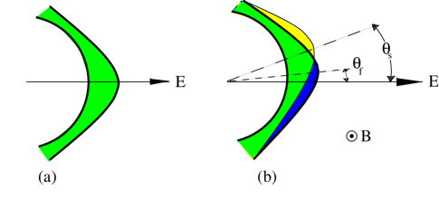
FIG. 5.: (a) Application of field creates a mixture of slowly and rapidly relaxing quasiparticles. (b) Slow and fast component of the Majorana fluid precesses in a field, developing their own Hall angle $\theta_{s,f}=\omega_{c}/\Gamma_{s,f}$.

A simple physical picture of the effect of an electric field is provided in Fig. 5. When an electric field is applied, it produces an admixture of $C=+1$ and $C=-1$ quasiparticles whose joint relaxation rate $\Gamma_{tr}=\frac{1}{2}[\Gamma_{s}+\Gamma_{f}]\approx\frac{1}{2}\Gamma_{f}$ is dominated by the rapidly relaxing quasiparticles. Magnetic fields couple diagonally to the Majorana quasi-particles, causing fast and slow components to develop their own Hall angle $\theta_{s,f}=\omega_{c}/\Gamma_{s,f}$ (Fig. 5). Since $\theta_{s}\gg\theta_{f}$, the Hall current is entirely dominated by the slow-relaxation quasiparticles. This has the effect of producing a finite magneto-resistance, even for isotropic Fermi surfaces: $\frac{\Delta\rho}{\rho}=\tan^{2}\theta_{H}$.

For completeness we also include in our table the thermal transport conductivities. Of these, the thermo-power and thermal conductivity have been most studied. A thermal gradient couples diagonally to the quasiparticles, so thermal and thermo-electric conductivities are determined by the slow relaxation rate. The difference in the relaxation times of the electrical and thermo-electric currents then gives rise to the unique temperature independent component in the Seebeck coefficient $S=-\rho\beta\propto(T\Gamma_{f}/\Gamma_{s})$ as we have already indicated. We can not compare our prediction of the thermal conductivity to experiment since we are unable to extract the large phonon contribution. Magneto-thermal measurements are still at an early stage but these are included in the table where results have been published.

Thus far we have neglected spin. In the absence of a measurement of the “spin conductivity” it is not clear which scattering rate will dominate this quantity. By choosing eigenstates of $C$ we have developed a phenomenology in which spin currents decay with the slow relaxation rate—spin-charge decoupling. However, if eigenstates of $CPT$ were used then in addition to the results already derived we would have a phenomenology where spin currents and electric currents decay with the fast rate.

Finally, the results derived here may be extended to finite frequency by the replacement $\Gamma_{f}\rightarrow\Gamma_{f}(\omega)-i\omega$, $\Gamma_{s}\rightarrow\Gamma_{s}(\omega)-i\omega$. Detailed fits to experiment require a knowledge of the frequency dependence of the relaxation rates and therefore a microscopic model. However, at low frequencies we may assume that relaxation rates are frequency independent and so optical measurements provide an important check on our phenomenology. For the A.C. Hall conductivity $\sigma_{xy}(\omega)$ our model predicts

$$\tan\theta_{H}(\omega)={\sigma_{xx}(\omega)\over\sigma_{xy}(\omega)}={\omega_{c}\over 2}\left({1\over\Gamma_{f}-i\omega}+{1\over\Gamma_{s}-i\omega}\right)\;,$$ (86)

There is thus a slow, and a fast component to the Hall relaxation. At low frequencies $\omega\ll\Gamma_{f}$,

$$\cot\theta_{H}(\omega)\sim 2\left({\Gamma_{s}(T)-i\omega\over\omega_{c}}\right),\quad\ (\Gamma_{s},\ \omega\ll\Gamma_{f})\;.$$ (87)

In particular $Im[\cot\theta_{H}(\omega)]\sim\omega/\omega_{c}$ is predicted to be temperature independent. This should be contrasted with the skew-scattering model,[17] where $\omega_{c}\rightarrow\omega_{c}^{*}(T)\propto{1\over T}$ is renormalized and there is only one relaxation rate $\Gamma_{s}=\Gamma_{f}$. In this case, $Im[\cot\theta(\omega)]\propto\omega T$ is proportional to temperature.

Recent optical measurements on $YBCO$ films by Drew et. al. have furnished results qualitatively in accord with Eq. 87.[13] When the sample becomes superconducting, a flux-lattice pinning mode develops in the optical Hall angle, with roughly twice the spectral weight found at frequencies below $\sim 200{\rm cm}^{-1}$ in the normal state. Our model can account for this feature in terms of the additional, high frequency Hall relaxation at frequencies $\omega\sim\Gamma_{tr}$. If the additional spectral weight in the high frequency component condenses into the flux lattice response, we expect a doubling of the transverse spectral weight. One of the difficulties that these measurements present us with, is that $\Gamma_{s}$ is only a factor of $4$ times smaller than $\Gamma_{f}$. It is not clear at present, whether this is due to disorder in the thin-films used, or whether this constitutes a significant discrepancy with our phenomenology. It would be very interesting in this respect, to have a direct measurement of the temperature dependence of $\Gamma_{s}$, which is not, at present available.

V Microscopic Implications.

We now return to address some of the key microscopic issues that were skirted in the phenomenology of the previous sections. We have been led by symmetry arguments to propose an electron relaxation rate that depends on the charge-conjugation operator

$$\underline{\Gamma}=\Gamma_{1}+\Gamma_{2}{\rm\hat{C}},$$ (88)

so that the even- and odd-parity charge-conjugation eigenstates decay at different rates. Each time the charge-conjugation operator acts, the following units of charge and momentum are transferred from the quasiparticle to its environment

$$\Delta Q=\pm 2e,\qquad\Delta\vec{P}=\pm 2\vec{k}_{F}.$$ (89)

In other words, we require a metallic environment where the electrons or holes can emit low energy quanta of momentum and charge. The phenomenology we have developed is, in essence a mean-field theory where these low-energy quanta are treated as condensed excitations.

A closely analogous situation does occur in the presence of superconducting fluctuations. A Boguilubov quasiparticle at the Fermi energy

$$\alpha{{}^{{\dagger}}}_{\rm\vec{k}_{F}}|\Phi\rangle=\frac{1}{\sqrt{2}}(c{{}^{{\dagger}}}_{\rm\vec{k}_{F}\uparrow}+c_{\rm-\vec{k}_{F}\downarrow})|\Phi\rangle$$ (90)

is an even-parity eigenstate of $CP$. In the presence of superconducting fluctuations, the relaxation rates of the eigenstates of $CP$ differ. Calculations by Aronov, Hikami and Larkin (AHL) confirm this conclusion: the conductivity contains an enhancement due to superconducting fluctuations

$$\sigma_{xx}\rightarrow\sigma_{xx}(1+\lambda),$$ (91)

and the Hall angle is depressed by the same factor

$$\theta_{H}\rightarrow\theta_{H}(1-\lambda),$$ (92)

Since the conductivity and the Hall angle satisfy optical sum rules, in the presence of superconducting fluctuations the transport relaxation rate is reduced but the Hall relaxation rate is enhanced,

$$\Gamma_{\rm tr} \rightarrow \Gamma_{\rm tr}(1-\lambda),$$ (93)

$$\Gamma_{H} \rightarrow \Gamma_{H}(1+\lambda),$$ (94)

An appropriate generalization of Landau Ginsburg theory, where the order-parameter carries momentum, is the “Brazovskii model”, [27] with the action

$${\cal F} = \int d^{d}x\left\{\frac{a}{2}|\psi|^{2}+\frac{b}{4!}|\psi|^{4}+{\xi_{o}^{4}\over 2}|\bigl{[}{p\kern-4.73611pt\raise-0.86108pt\hbox{/}}^{2}-(2k_{F})^{2}\bigr{]}\Psi|^{2}\right\},$$ (95)

$${p\kern-4.73611pt\raise-0.86108pt\hbox{/}} = -i\hbar\vec{\nabla}-2e\vec{A}\;,$$ (96)

where the pair fluctuations are staggered. An extension of the AHL calculation to this case is expected to to show an enhanced current relaxation rate, and a depressed Hall relaxation rate.

One of the interesting questions raised by this discussion, is whether there might be a microscopic link between our phenomenology and spin-charge decoupling.[3] There are two fascinating links that should be mentioned here. Firstly, the holon in a Luttinger liquid is a charge carrying excitation with a definite momentum. Holon emission would give rise to “electron oscillations”: fluctuations between degenerate electron and hole states on the same side of the Fermi surface of the form

$$e^{-}\rightleftharpoons{\rm spinon\ state}\rightleftharpoons h^{+},$$ (97)

which would generate the time-scale separation that we have been discussing. This would be the a direct analog of the processes that give rise to Kaon oscillations[28] in particle physics. Secondly, although the holon is charged, since it is not possible to assign a well-defined sign to the charge of a holon, both the spinon and the holon should be regarded as  charge-conjugation eigenstates. In other-words, spin-charge decoupling may naturally lead to quasiparticles that are charge-conjugation eigenstates, a condition we need for two relaxation time-scales.

Before describing our attempts to make a passage to a more microscopic theory, let us summarize the key questions that have to be addressed:

  $\bullet$

What is the nature of the low energy charged excitations that mix electrons and holes, and how does this excitation couple to the original electron fields to produce the anomalous scattering described above?

  $\bullet$

What are the dynamics of the charged excitation, and how is it possible to produce something with a correlation length that exceeds the electron mean-free path, but does not diverge to macroscopic lengths, over a very wide range of temperatures?

We should like to end by sketching our attempt to address these questions. We have tried to link our phenomenology with the other non-Fermi liquid properties of the cuprate metallic state. Optical conductivity measurements show that the phase angle of the conductivity is almost constant up to 1eV, a feature which suggests that the electron self-energies have a singular energy dependence out to high energies.[29] The appearance of a linear transport relaxation rate around the Fermi surface of the cuprates has been used to argue that the electron-self energy has a “marginal” form[30]

$$\Sigma(\omega)\propto\omega{\rm ln}\biggl{[}{\rm max}(\omega,T)\biggr{]}\;,$$ (98)

where ${\rm max}(\omega,T)$ is an analytic function with asymptotes given by $\omega$, or $T$, which-ever is bigger. A self-energy with this particular structure is unusual even in the context of non-Fermi liquid models. For example, in a 1D Tomonaga-Luttinger liquid, the self-energy has the form $\Sigma(\omega)\sim\omega^{\alpha}$, where $\alpha$ depends on the interactions.

There is a way in which the two-relaxation time scenario can be unified with the marginal Fermi liquid picture. Let us suppose that the marginal scattering is highly retarded, so that the momentum-dependence of the self-energy can be ignored in our discussion. Since the marginal self-energy is scale invariant, we expect it to obey a simple power-law in the time domain. By power-counting, it follows that

$$\Sigma(t)\propto{\rm 1\over t^{2}}{\rm sgn}(t)\;.$$ (99)

We identify $\Sigma(t)$ as the time-dependence of the three-body amplitude for the intermediate three-body state formed in electron-electron scattering. The local propagator of electrons in the Fermi sea has the form $G(t)\sim{\rm 1\over t}$. In a Fermi liquid $\Sigma(t)\sim[G(t)]^{3}\sim t^{-3}$. In a marginal Fermi liquid, the intermediate three-body state can be written in the suggestive form

$$\Sigma(\tau)=\lambda^{2}G(\tau)^{2}\left[{1\over 2}{\rm sgn}(\tau)\right].$$ (100)

We interpret the additional term on the right-hand-side as a zero-energy Fermionic excitation, without internal dynamics, as shown in Fig. 6(a).

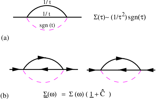
FIG. 6.: (a) Three-body bound-state interpretation of the marginal self-energy; (b) in order that the bound-state splits the degeneracy between the electric and Hall relaxation time, it must be a state of definite charge conjugation symmetry, which then generates normal and anomalous components of the self-energy of equal weight.

This hypothetical excitation may be represented by a single Fermi field $\Phi$, with propagator

$$G^{(0)}_{\Phi}(\vec{x}-\vec{x}^{\prime},\tau)={1\over 2}\delta(\vec{x}-\vec{x}^{\prime}){\rm sgn}(\tau).$$ (101)

In the frequency domain

$$G^{0}_{\Phi}(\vec{k},\omega)={1\over\omega}\;.$$ (102)

The possibility that such a three-body excitation might drive marginal Fermi liquid behavior was first considered by Ruckenstein and Varma. [31] In its original form, the three-body hypothesis did not explain why such a resonance is pinned to the Fermi energy. Generically, a fermionic mode at the Fermi energy will develop a self-energy that tends to repel it from the Fermi energy, eliminating the scale-invariance which is fundamental to the marginal scattering.

The arguments of the previous sections suggest an intriguing unified solution to this problem. Experiment tells us that the marginal scattering rate selectively relaxes the electrical current: we have argued that to do this, the marginal scattering must occur in a channel with a definite charge conjugation symmetry. If this is the case, then the hypothetical three-body bound-state must have a definite charge-conjugation parity. We are free to take this parity to be positive, so that

$$\Phi{{}^{{\dagger}}}(x)=C{{}^{{\dagger}}}\Phi(x)C=+\Phi(x)\;.$$ (103)

Such a state would immediately open up a decay mode of the form

$${\rm e}^{-}\rightleftharpoons({\rm e}^{-}{\rm h}^{+}\Phi)\rightleftharpoons{\rm h}^{+},$$ (104)

which would then cause the $C=+1$ eigenstates of the electron fluid $\frac{1}{\sqrt{2}}({\rm e}^{-}+{\rm h}^{+})$ to decay more rapidly than their $C=-1$ counterparts. In the language of spin-charge decoupling mentioned above, the intermediate state might be identified with the spinon.

This hypothetical $\Phi$ fermion that mediates electron oscillations is automatically particle-hole symmetric. Furthermore, the momentum-independent part of its self-energy $\Sigma_{\Phi}(\omega)$ is necessarily an odd-function of frequency, $\Sigma_{\Phi}(\omega)=-\Sigma_{\Phi}(-\omega)$. The $\Phi$ fermion couples to the conduction electrons, to develop a self-energy $\Sigma_{\Phi}(\tau)\propto 1/\tau^{3}$, so that $Im\Sigma_{\Phi}(\omega)\propto\omega^{2}$ at low frequencies, which means that local decay processes do not broaden the sharpness of this resonance. The only way such a mode can develop a width is through the development of coherent coupling between different sites. In the absence of coherence, the momentum dependence of $\Sigma_{\Phi}$ can be neglected so the the sharp pole in its propagator is preserved. i.e, if

$$G_{\Phi}^{0}({\omega})\longrightarrow G_{\Phi}({\omega})={1\over\omega-\Sigma_{\Phi}({\omega})},$$ (105)

then

$${1\over\pi}{\rm Im}\bigl{[}G_{\Phi}({\omega})\bigr{]}=Z\delta({\omega})+({\rm background})\;,$$ (106)

where $Z^{-1}=[1-\delta_{{\omega}}\Sigma_{\Phi}({\omega})]|_{0}$.

A three-body bound-state with definite charge-conjugation symmetry arises in the two-channel Kondo model, where it is a consequence of channel-symmetry. [32] In our case, the singular scattering derives from a spontaneous formation of these bound-states, presumably at energies around $1.0$eV, where the phase angle of the optical conductivity becomes constant. We can use this idea to make the marginal self-energy more precise. Let us generalize the form of Eq. 100 to finite temperatures, writing

$$G(\tau)={\pi\rho T\over\sin(\pi T\tau)}\;,$$ (107)

where $\rho$ is the density of states. Fourier transforming this we may derive the frequency dependent self-energy as follows

$$\Sigma(i\omega_{n})={i\over 2\beta}\int_{\Lambda^{-1}}^{\beta-\Lambda^{-1}}\sin{\omega_{n}\tau}\left[{\lambda\pi\rho T\over\sin(\pi T\tau)}\right]^{2},$$ (108)

where $\Lambda$ is a cut-off. Carrying out the integral and analytically extending to real frequencies, we obtain

$${1\over\tilde{\lambda}^{2}}\Sigma(\omega-i\delta)=-\omega\left[{\rm ln}{\tilde{\Lambda}\over T}-\Psi\left(1+{i\omega\over 2\pi T}\right)\right]+i\pi T\;,$$ (109)

where $\tilde{\Lambda}=\Lambda e^{1-C}/2\pi$ and $\tilde{\lambda}=\lambda\rho$. This function has imaginary part

$$\Lambda(\omega)={\lambda^{2}\omega\over 2}\coth\bigl{[}{\omega\over 2T}\bigr{]}\;.$$ (110)

Scale invariant marginal Fermi liquid behavior thus has a unique cross-over from high to low frequencies.

Let us now discuss the hypothetical interaction vertex illustrated in Fig. 6. How can a three-body bound-state interact selectively with only one component of the Fermi sea? To bring out the gauge invariance of the problem, we need a slightly more general definition of the Majorana fermions around the Fermi surface. If we write the conduction electrons in terms of the following matrix spinor

$$\Psi_{\rm\vec{p}}=\left[\begin{array}[]{rcl}\psi_{\rm\vec{p}\uparrow}&-\psi_{\rm-\vec{p}^{*}\downarrow}\cr\psi{{}^{{\dagger}}}_{\rm-\vec{p}\downarrow}&\psi{{}^{{\dagger}}}_{\rm\vec{p}^{*}\uparrow}\end{array}\right]\;,$$ (113)

then we can make a decomposition into Majorana fermions as follows

$$\Psi_{\rm\vec{p}}={1\over\sqrt{2}}(\psi^{0}_{\rm\vec{p}}+i\vec{\psi}_{\rm\vec{p}}\cdot\vec{\tau}).$$ (114)

We can define coarsely-localized Majorana fermions by taking the Fourier transform of these quantities

$$\psi^{(a)}(x)=\sum_{\{\rm\vec{p}\}}\psi^{(a)}_{\rm\vec{p}}e^{i\rm\vec{p}\cdot\vec{x}}\;,$$ (115)

where the momentum sum is taken within a narrow shell around the exterior of the Fermi surface.

The existence of a Majorana bound-state, amounts to the assumption that three-body correlations are governed by the following contractions

$$\mathrel{\mathop{{\psi^{(1)}(x)\psi^{(2)}(x)\psi^{(3)}(x)}}^{\displaystyle\raise-1.8pt\hbox{$\scriptscriptstyle|$}\mathrel{\mkern-10.0mu}\mathrel{{\bf\smash{{\phantom{-}\above 1.0pt\phantom{-}}}}}\mathrel{\mkern-11.0mu}\mathrel{{\bf\smash{{\phantom{-}\above 1.0pt\phantom{-}}}}}\mathrel{\mkern-11.0mu}\mathrel{{\bf\smash{{\phantom{-}\above 1.0pt\phantom{-}}}}}\mathrel{\mkern-11.0mu}\mathrel{{\bf\smash{{\phantom{-}\above 1.0pt\phantom{-}}}}}\mathrel{\mkern-11.0mu}\mathrel{{\bf\smash{{\phantom{-}\above 1.0pt\phantom{-}}}}}\mathrel{\mkern-12.0mu}\mathrel{{\bf\smash{{\phantom{-}\above 1.0pt\phantom{-}}}}}\mathrel{\mkern-12.0mu}\mathrel{{\bf\smash{{\phantom{-}\above 1.0pt\phantom{-}}}}}\mathrel{\mkern-12.0mu}\mathrel{{\bf\smash{{\phantom{-}\above 1.0pt\phantom{-}}}}}\mathrel{\mkern-12.0mu}\raise-1.8pt\hbox{$\scriptscriptstyle|$}\mathrel{\mkern-9.0mu}\mathrel{{\bf\smash{{\phantom{-}\above 1.0pt\phantom{-}}}}}\mathrel{\mkern-11.0mu}\mathrel{{\bf\smash{{\phantom{-}\above 1.0pt\phantom{-}}}}}\mathrel{\mkern-11.0mu}\mathrel{{\bf\smash{{\phantom{-}\above 1.0pt\phantom{-}}}}}\mathrel{\mkern-11.0mu}\mathrel{{\bf\smash{{\phantom{-}\above 1.0pt\phantom{-}}}}}\mathrel{\mkern-11.0mu}\mathrel{{\bf\smash{{\phantom{-}\above 1.0pt\phantom{-}}}}}\mathrel{\mkern-10.0mu}\mathrel{{\bf\smash{{\phantom{-}\above 1.0pt\phantom{-}}}}}\mathrel{\mkern-10.0mu}\mathrel{{\bf\smash{{\phantom{-}\above 1.0pt\phantom{-}}}}}\mathrel{\mkern-9.5mu}\raise-1.8pt\hbox{$\scriptscriptstyle|$}}}=\lambda\Phi(x)\;.$$ (116)

If we want to be more general, we can write

$$\mathrel{\mathop{{\psi^{(a)}(x)\psi^{(b)}(x)\psi^{(c)}(x)}}^{\displaystyle\raise-1.8pt\hbox{$\scriptscriptstyle|$}\mathrel{\mkern-10.0mu}\mathrel{{\bf\smash{{\phantom{-}\above 1.0pt\phantom{-}}}}}\mathrel{\mkern-11.0mu}\mathrel{{\bf\smash{{\phantom{-}\above 1.0pt\phantom{-}}}}}\mathrel{\mkern-11.0mu}\mathrel{{\bf\smash{{\phantom{-}\above 1.0pt\phantom{-}}}}}\mathrel{\mkern-11.0mu}\mathrel{{\bf\smash{{\phantom{-}\above 1.0pt\phantom{-}}}}}\mathrel{\mkern-11.0mu}\mathrel{{\bf\smash{{\phantom{-}\above 1.0pt\phantom{-}}}}}\mathrel{\mkern-12.0mu}\mathrel{{\bf\smash{{\phantom{-}\above 1.0pt\phantom{-}}}}}\mathrel{\mkern-12.0mu}\mathrel{{\bf\smash{{\phantom{-}\above 1.0pt\phantom{-}}}}}\mathrel{\mkern-12.0mu}\mathrel{{\bf\smash{{\phantom{-}\above 1.0pt\phantom{-}}}}}\mathrel{\mkern-12.0mu}\raise-1.8pt\hbox{$\scriptscriptstyle|$}\mathrel{\mkern-9.0mu}\mathrel{{\bf\smash{{\phantom{-}\above 1.0pt\phantom{-}}}}}\mathrel{\mkern-11.0mu}\mathrel{{\bf\smash{{\phantom{-}\above 1.0pt\phantom{-}}}}}\mathrel{\mkern-11.0mu}\mathrel{{\bf\smash{{\phantom{-}\above 1.0pt\phantom{-}}}}}\mathrel{\mkern-11.0mu}\mathrel{{\bf\smash{{\phantom{-}\above 1.0pt\phantom{-}}}}}\mathrel{\mkern-11.0mu}\mathrel{{\bf\smash{{\phantom{-}\above 1.0pt\phantom{-}}}}}\mathrel{\mkern-10.0mu}\mathrel{{\bf\smash{{\phantom{-}\above 1.0pt\phantom{-}}}}}\mathrel{\mkern-10.0mu}\mathrel{{\bf\smash{{\phantom{-}\above 1.0pt\phantom{-}}}}}\mathrel{\mkern-9.5mu}\raise-1.8pt\hbox{$\scriptscriptstyle|$}}}=\lambda\epsilon^{abcd}g_{d}(x)\Phi(x)\;,$$ (117)

where $g_{d}(x)$ is a four-component vector that describes the wave-function of the bound-state. Similar types of three-body correlation have been considered in the context of odd-frequency pairing correlations.[33, 34]

These considerations motivate us to consider interaction vertices of the form

$$H_{I}=\sum_{x}\epsilon^{abcd}g_{d}(x)\Phi(x)\psi^{(a)}(x)\psi^{(b)}(x)\psi^{(c)}(x)\;,$$ (118)

as a possible common origin of marginal Fermi liquid behavior and two relaxation times. The quantity $g_{d}(x)$ is to be regarded as a slowly varying order parameter that describes the collective emission of charged excitations. If we rotate to a basis where $g=\frac{1}{6}(\lambda,0,0,0)$, locally the interaction takes the form

$$H_{I}=\lambda\sum_{x}\Phi(x)\psi^{(1)}(x)\psi^{(2)}(x)\psi^{(3)}(x)\;,$$ (119)

so that the three “vector” components of the conduction sea develop a marginal self-energy, whereas the one remaining component $\psi^{(0)}(x)$ would not couple to the bound-state, thereby preserving a more conventional Fermi liquid self-energy. In order for this picture to work, it is necessary to assume that the three-body wave-function, $g(x)$ has a coherence length that is large compared with electron mean-free paths. One of the interesting challenges, is to see whether the optical conductivity and Hall conductivity predicted by such a phenomenology is in accord with experiment.

At present, these ideas are incomplete and under closer scrutiny they suffer from a number of difficulties. In particular,

1. The description is incomplete without a Lagrangian for the three-body amplitude, $g(x)$. It is difficult to see how to construct such a Lagrangian in a fashion that will preserve both charge and momentum conservation.

2. What is the nature of the charged excitation represented by $g(x)$? It is tempting to identify this object with the “holons” entering into Anderson’s Luttinger liquid scenario.

3. Why does the boson represented by $g(x)$ not short-circuit the conductivity at low temperatures, like a super-current?

4. If the three-body bound-state is a local object, then what possible aspect of the local quantum chemistry could give rise to it? Contrariwise, if the bound-state is rather extended in real space, then what aspect of the Fermi surface would give rise to its spontaneous formation?

Though we are clearly far from a microscopic explanation of the two-relaxation times, we expect certain broad features of our discussion to remain robust. We have demonstrated that experimental results, combined with the use of the transverse optical sum rule, strongly support the presence of two independent relaxation time scales for the Hall and electric current. This kind of separation between relaxation rates, if confirmed, indicates that the underlying quasiparticles must be states of definite charge conjugation parity. Such a separation can not occur without the presence of some, as yet unidentified, low energy excitation that carries both current and momentum.

We have discussed the possible origin of this separation. One possibility is the presence of staggered superconducting fluctuations. Another, not necessarily unrelated idea, is the possibility that what we are seeing here is some form of spin-charge separation. In this case, the low-lying charge excitations of definite charge conjugation parity might be identified with the holons of a Luttinger liquid. Finally, we have described how the presence of a zero-energy fermionic mode with definite charge conjugation symmetry may provide a way to unify these ideas with the idea of a marginal Fermi liquid. These ideas may not be mutually exclusive. Careful experiment, especially more accurate optical conductivity measurements clearly have a central role to play in elucidating these issues.

We should like to thank E. Abrahams, P. W. Anderson, H. D. Drew, D. E. Khmelnitskii, G. L. Lonzarich and Ph. Ong for discussions related to this work. This research was supported by travel funds from NATO grant CRG 940040 (AMT & PC), NSF grants DMR-93-12138 (PC) and DM-92-21907 and a travel fellowship from the Royal Society (AJS).

A Diagrammatics for the Hall effect

This section summarizes the conventional calculation of the Hall conductivity, following the approach of Voruganti et al.[18] Throughout, we assume an $s$-wave scattering potential which avoids the need to consider vertex corrections.

For spin-less electrons with dispersion $\epsilon(\vec{p})\equiv\epsilon_{\vec{p}}$, the Hamiltonian in the presence of a vector potential is given by

$$H=\sum_{\rm\vec{p}}\psi^{\dagger}_{\rm\vec{p}}\epsilon[\rm\vec{p}-e\vec{A}(x)]\psi_{\rm\vec{p}}\;.$$ (A1)

where $\vec{x}=i\nabla_{\vec{p}}$ is the position operator and $\vec{A}$ is an external vector potential that varies slowly on macroscopic length-scales. The field dependent part of the action, $S_{A}$, can be systematically in powers of $\vec{A}$ as follows

$${\cal S}_{A} = \sum_{n=1}^{\infty}{(-e)^{n}\over n!}\epsilon^{\alpha_{1}\cdots\alpha_{n}}_{\vec{p}}\biggl{(}A^{\alpha_{1}}_{{\vec{q}}_{1}}\cdots A^{\alpha_{n}}_{{\vec{q}}_{n}}\biggr{)}\psi^{\dagger}_{{\vec{p}^{+}}}\psi_{{\vec{p}^{-}}}$$ (A2)

$$= e\epsilon^{\alpha}_{\vec{p}}A^{\alpha}_{\vec{q}}\psi^{\dagger}_{{\vec{p}}+{{\vec{q}}\over 2}}\psi_{{\vec{p}}-{{\vec{q}}\over 2}}$$ (A4)

$$+{e^{2}\over 2}\epsilon^{\alpha\beta}_{\vec{p}}A^{\alpha}_{\vec{k}}A^{\beta}_{\vec{q}}\psi^{\dagger}_{{\vec{p}}+{{\vec{k}}\over 2}+{{\vec{q}}\over 2}}\psi_{{\vec{p}}-{{\vec{k}}\over 2}-{{\vec{q}}\over 2}}+\cdots$$

where repeated 4-momenta and indices are summed over, $\vec{p}^{\pm}=\vec{p}\pm\sum_{j}\vec{q}_{j}/2$ and

$$\epsilon^{\alpha_{1}\cdots\alpha_{n}}_{\rm\vec{p}}={\nabla_{p^{\alpha}_{1}\cdots p^{\alpha}_{n}}}\epsilon(\rm\vec{p})\;.$$ (A5)

The current operator is determined from

$$J^{\alpha}_{q}=-{1\over V}{\partial{\cal S}_{A}\over\partial A^{\alpha}_{-q}}.$$ (A6)

We wish to determine the current response to a uniform electric and static magnetic field. The vector potential can be divided up into two components

$$\vec{A}(\vec{r},t)=\vec{a}^{E}(\vec{r},t)+\vec{a}^{H}(\vec{r})$$ (A7)

where the time-dependent term gives rise to the electric field $\vec{E}=-i\nu\vec{a}^{E}_{\nu}$, and the static term $\vec{a}^{H}$ determines the magnetic field, $\vec{H}=-i\vec{q}\times\vec{a}^{H}_{\vec{q}}$. For simplicity, we shall concentrate on a single frequency $\nu$, and momentum $\pm\vec{q}$, where $\vec{q}$ $\vec{q}$ is ultimately set to zero. The electrical and Hall conductivity are obtained by determining the current response as a power series in $\vec{A}$. Gauge invariance seriously reduces the numbers of diagrams which contribute to the conductivity at a given order(see Ref. [18]).

To first order in $\vec{A}$, we expect currents proportional to $\vec{E}$ and $\vec{H}$:

$$\vec{J}=\sigma\vec{E}+\chi\vec{\nabla}\times\vec{H}\;,$$ (A8)

which correspond to diagrams proportional to $-i\nu\vec{a}^{E}_{q,\nu}$ and $q^{2}\vec{a}^{H}_{q}$ . For the conductivity we may limit our attention to diagrams proportional to $i\nu a^{E}$. The only frequency dependent diagram, is the “bubble” diagram, illustrated in Fig. 7a. The conductivity is thus given by

$$\sigma_{xx}(\nu)={e^{2}\over-i\nu}\sum_{\vec{p}}(\epsilon^{x}_{\vec{p}})^{2}{\Lambda}(\vec{p},\nu)\;,$$ (A9)

where,

$${\Lambda}(\vec{p},i\nu_{n})={1\over\beta}\sum_{\omega_{r}}{\cal G}^{(+)}_{\vec{p}}\bigl{[}{\cal G}^{(-)}_{\vec{p}}-{\cal G}^{(+)}_{\vec{p}}\bigr{]}.$$ (A10)

Here we have used the notation ${\cal G}^{(\pm)}_{\vec{p}}\equiv{\cal G}(\vec{p},i\omega_{r}^{\pm})$ and $\omega_{r}^{\pm}=\omega_{r}\pm\nu_{n}/2$. For frequencies far smaller than the Fermi energy, the Matsubara sums give rise to a function that is quite sharply peaked in the vicinity of the Fermi surface. This permits us to replace the momentum sum by an energy integral as follows

$$\sum_{\vec{p}}(\epsilon^{x}_{\vec{p}})^{2}{\Lambda}(\vec{p},i\nu_{n})\rightarrow$$ (A11)

$${n\over m}\int_{-\infty}^{\infty}d\epsilon{1\over\beta}\sum_{\omega_{r}}{\cal G}^{(+)}_{\epsilon}\bigl{[}{\cal G}^{(-)}_{\epsilon}-{\cal G}^{(+)}_{\epsilon}\bigr{]}.$$ (A12)

where ${\cal G}_{\epsilon}(\omega_{n})=[i\omega_{n}-\epsilon_{\vec{p}}+\frac{i}{2}\Gamma{\rm sgn}(\omega_{n})]^{-1}$ is the electron propagator with a phenomenological relaxation rate $\Gamma$, and we have assumed a parabolic band to replace the angular average as follows $<v_{x}^{2}>N(0)\rightarrow n/m$.

Carrying out the energy integral as a contour integral then gives

$$\sum_{\vec{p}}(\epsilon^{x}_{\vec{p}})^{2}{\Lambda}(\vec{p},i\nu_{n})={n\over m}{\nu_{n}\over\Gamma+\nu_{n}}.$$ (A13)

where we have taken $\nu_{n}>0$. Extending this result to real frequencies recovers the classic relaxation time approximation

$$\sigma_{xx}(\nu+i\delta)={ne^{2}\over m}{1\over\Gamma-i\nu}.$$ (A14)

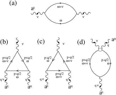
FIG. 7.: (a) The sole diagram contributing to the electrical conductivity while (b)(c) and (d) show the terms contributing to the Hall conductivity.

In an isotropic system, the second-order response determines the Hall current, which is proportional to $\vec{E}\times\vec{H}$. In terms of the vector potential the uniform component of the Hall current must have the following form

$$j_{H}(\nu)\propto\nu\vec{a}^{E}({-\vec{q}})\times\bigl{[}\vec{q}\times\vec{a}^{H}({\vec{q}})\bigr{]}.$$ (A15)

There are six second-order diagrams proportional to $a^{E}(-q,\nu)a^{H}(q)$, but gauge-invariance tells us that all terms must cancel excepting those which depend on a product of both $\nu$ and $q$. These diagrams are illustrated in Fig. 7(b-d). We can further simplify things by directly extracting the leading $q$ dependence. Adding the two triangle diagrams Fig. 7(b-c). we find that the terms proportional to $q$ obtained by expanding the Greens functions cancel, and the only residual $q$ dependence comes from expanding the vertex $\epsilon^{\alpha}_{k\pm q/2}\rightarrow\epsilon^{\alpha}_{k}\pm q^{\beta}\epsilon^{\alpha\beta}_{k}/2$. The leading $q$ dependence of Fig. 7(c). is obtained by expanding the Green’s functions in the bubble: ${\cal G}(k\pm q/2)\rightarrow{\cal G}(k)\pm q^{\beta}\epsilon^{\beta}_{k}{\cal G}(k)^{2}$. The sum of these contributions is represented by the triangle diagrams shown in Fig. 2b. The evaluation of these two diagrams leads to

$$\sigma_{xy}(\nu)={e^{3}H\over\nu}\sum_{\vec{k}}\left(\epsilon^{x}_{\vec{k}}\epsilon^{x}_{\vec{k}}\epsilon^{yy}_{\vec{k}}-\epsilon^{x}_{\vec{k}}\epsilon^{y}_{\vec{k}}\epsilon^{xy}_{\vec{k}}\right)\Pi(\vec{k},\nu)$$ (A16)

where

$$\Pi(\vec{k},i\nu_{r})={1\over 2\beta}\sum_{\omega_{n}}{\cal G}^{(+)}_{\vec{k}}{\cal G}^{(-)}_{\vec{k}}\left[{\cal G}^{(-)}_{\vec{k}}-{\cal G}^{(+)}_{\vec{k}}\right].$$ (A17)

In the Landau gauge, where $\vec{a}^{H}=(a^{H},0,0)$ and $\vec{q}=(0,q,0)$, the first term in (A16) is obtained from the triangle diagrams Fig. 7(b-c), whereas the second term comes from the q-expansion of the bubble diagram Fig. 7(d). For a parabolic band, the second term vanishes, so we could have completely neglected the bubble diagrams. As in the case of the conductivity, the Matsubara summations lead to a function that is quite sharply peaked within a few $kT$ of $\epsilon(k_{F})$ , so the momentum sum only probes the region close to the Fermi surface and the momentum sum can then be replaced by an energy integral as follows

$$\sigma_{xy}(i\nu_{n})={ne^{3}H\over i\nu_{n}m^{2}}{1\over 2\beta}\sum_{r}\tilde{\Pi}(i\omega_{r}^{+},i\omega_{r}^{-})$$ (A18)

and

$$\tilde{\Pi}(i\omega_{r}^{+},i\omega_{r}^{-})=\int_{-\infty}^{\infty}d\epsilon{\cal G}^{(+)}_{\epsilon}{\cal G}^{(-)}_{\epsilon}\bigl{[}{\cal G}^{(-)}_{\epsilon}-{\cal G}^{(+)}_{\epsilon}\bigr{]}.$$ (A19)

where we have used the shorthand notation ${\cal G}^{(\pm)}_{\epsilon}\equiv{\cal G}(\epsilon,i\omega_{r}^{\pm})$. Carrying out the energy integral then gives

$$\tilde{\Pi}(i\omega_{r}^{+},i\omega_{r}^{-})={\pi i\over(\Gamma+\nu_{n})^{2}}[\Theta(\omega_{r}^{+})-\Theta(\omega_{r}^{-})],$$ (A20)

so that

$$\sigma_{xy}(\nu+i\delta)={ne^{2}\over m}{\omega_{c}\over(\Gamma-i\nu)^{2}},$$ (A21)

recovering the result of Boltzmann transport theory.

B Diagrammatics with charge-conjugation eigenstates

We now build on the experience gained in Appendix A and repeat the calculation using charge-conjugation eigenstates and a phenomenological scattering rate which depends on the charge conjugation parity. We begin by combining electron states above the Fermi surface with their charge-conjugation partners below it to make a spinor

$$\Psi_{{\rm\vec{p}}\sigma}=\left(\begin{array}[]{rl}\psi_{{\rm\vec{p}}-\sigma}\cr\sigma\psi{{}^{{\dagger}}}_{{\rm\vec{p}^{*}}\sigma}\end{array}\right)\;.$$ (B3)

The Hamiltonian in a field is then

$$H_{o}=\displaystyle\sum_{{\rm|\vec{p}|>|\vec{p}_{F}|},\sigma}\Psi{{}^{{\dagger}}}_{{\rm\vec{p}}\sigma}{\rm\epsilon}_{{\rm\vec{p}-e\vec{A}\tau_{3}}}\Psi_{{\rm\vec{p}}\sigma}\;.$$ (B4)

where $\tau_{3}$ is the third Pauli spinor. The momentum sum is now restricted to outside the Fermi surface because the hole states are already included in the spinor. By differentiating with respect to the vector potential, we may derive the corresponding current operator

$${\cal J}=e\sum_{{\rm|\vec{p}|>|\vec{p}_{F}|},\sigma}\Psi{{}^{{\dagger}}}_{{\rm\vec{p}}\sigma}\bigl{[}{\rm\vec{v}_{\rm\hat{p}_{F}}\tau_{3}+\underline{m}^{-1}(\delta\vec{p}-e\vec{A}\tau_{3})}\bigr{]}\Psi_{{\rm\vec{p}}\sigma}\;.$$ (B5)

In this basis the electro-magnetic field is diagonal, but the states are not eigenstates of the $C$. To make the charge conjugation eigenstate, we make a rotation within the degenerate electron and hole states, writing

$${\tilde{\Psi}}_{\rm\vec{p}\sigma}=U\Psi_{\rm\vec{p}\sigma}$$ (B6)

where,

$$U=\left[\begin{array}[]{rl}{1\over\sqrt{2}}&{1\over\sqrt{2}}\cr{-i\over\sqrt{2}}&{i\over\sqrt{2}}\end{array}\right]\;,\qquad{\tilde{\Psi}}_{{\rm\vec{p}}\sigma}=\left(\begin{array}[]{rl}a_{{\rm\vec{p}}\sigma}\cr b_{{\rm\vec{p}}\sigma}\end{array}\right)\;,$$ (B7)

where $a$ and $b$ are defined in Eq. 57. The transformation to the new basis is easily effected by noting that

$$U\tau_{3}U{{}^{{\dagger}}}=\tau_{2},$$ (B8)

where $\tau_{2}$ is the second Pauli matrix. In the new basis, the Hamiltonian is thus

$$H_{o}=\displaystyle\sum_{{\rm|\vec{p}|>|\vec{p}_{F}|},\sigma}{\tilde{\Psi}}{{}^{{\dagger}}}_{{\rm\vec{p}}\sigma}{\rm\epsilon}_{{\rm\vec{p}-e\vec{A}\tau_{2}}}{\tilde{\Psi}}_{{\rm\vec{p}}\sigma}\;.$$ (B9)

and the current operator becomes

$${\cal J}=e\sum_{{\rm|\vec{p}|>|\vec{p}_{F}|},\sigma}\tilde{\Psi}{{}^{{\dagger}}}_{{\rm\vec{p}}\sigma}\bigl{[}{\rm\vec{v}_{\rm\hat{p}_{F}}\tau_{2}+\underline{m}^{-1}(\delta\vec{p}-e\vec{A}\tau_{2})}\bigr{]}\tilde{\Psi}_{{\rm\vec{p}}\sigma}\;.$$ (B10)

In the absence of an external field, this Hamiltonian is diagonal and charge-conjugation is a conserved symmetry.[35] Our phenomenological assumption is that the leading irrelevant interactions in this Hamiltonian yield independent lifetimes for the $a$ and $b$ particle:

$${\cal G}^{-1}_{a}(\vec{p},i\omega) = i\omega-\epsilon_{\vec{p}}+\frac{i}{2}\Gamma_{f}{\rm sign}(\omega)\;,$$ (B11)

$${\cal G}^{-1}_{b}(\vec{p},i\omega) = i\omega-\epsilon_{\vec{p}}+\frac{i}{2}\Gamma_{s}{\rm sign}(\omega)\;.$$ (B12)

where we have arbitrarily assigned the fast relaxation rate to the $a$ particle. The matrix propagator for $\tilde{\Psi}$ is then

$${\cal G}(\vec{p},i\omega)=\left[\begin{array}[]{rl}{{\cal G}_{a}(\vec{p},i\omega)}&{}\cr{}\hfil&{{\cal G}_{b}(\vec{p},i\omega)}\end{array}\right]$$ (B15)

In general $\Gamma_{f}$ and $\Gamma_{s}$ will be momentum and frequency dependent, however out of ignorance we assume that they are $p$ independent (so we don’t have vertex corrections). We will also consider them to be frequency independent, though this is an assumption that is readily relaxed.

It is straightforward to repeat the diagrammatic approach of Appendix B in this matrix formalism. Suppose for the moment we take a parabolic band and naively assume that bubble diagrams of the form Fig. 7(d) may be neglected, then we can restrict our attention to the triangle diagrams of the type shown in Fig. 7(b) & (c). From (B10), we see that we can quickly generalize the momentum-independent and momentum-dependent parts of the current vertices to the matrix notation by making the following substitutions

$$\vec{v}_{F} \longrightarrow \vec{v}_{F}\otimes\tau_{2},$$ (B16)

$$\underline{m}^{-1}_{\rm\vec{p}} \longrightarrow \underline{m}^{-1}_{\rm\vec{p}}\otimes\underline{1}.$$ (B17)

With these modifications, we find that results of Appendix A. may be generalized by writing

$$\Lambda(\vec{p},i\nu_{n}) = {1\over 2\beta}\sum_{\omega_{r}}{\rm Tr}\left[\tau_{2}\bigl{(}{\cal G}^{(+)}_{\vec{p}}-{\cal G}^{(-)}_{\vec{p}}\bigr{)}\tau_{2}{\cal G}^{(-)}_{\vec{p}}\right],$$ (B18)

$$\Pi(\vec{p},\nu) = {1\over 4\beta}\sum_{\omega_{n}}{\rm Tr}\left\{{\cal G}^{(+)}_{\vec{p}}{\cal G}^{(-)}_{\vec{p}}\tau_{2}\bigl{[}{\cal G}^{(-)}_{\vec{p}}-{\cal G}^{(+)}_{\vec{p}}\bigr{]}\tau_{2}\right\}$$ (B19)

where we have used the shorthand notation ${\cal G}^{(\pm)}_{\vec{p}}\equiv{\cal G}(\vec{p},i\omega_{r}\pm i\nu_{n}/2)$. These expressions revert to those given in Appendix A. when $\Gamma_{a}=\Gamma_{b}$. A simple diagrammatic interpretation of both expressions can be made by noting that $\tau_{2}$ is off-diagonal in the Majorana basis. The electric current operator is off-diagonal in this basis, and the Fermion bubble entering into the conductivity contains one “a” and one “b” propagator, as shown in Fig. 8(a). By contrast, the Hall conductivity involves the effective mass operator, which is diagonal in the “a-b” basis. The triangle diagrams entering into the Hall conductivity are shown in Fig. 8(b).

Replacing the momentum sums by an energy integral, we can repeat the steps of Appendix A., to find

$$\sum_{\vec{p}}(v^{x}_{\vec{p}_{F}})^{2}{\Lambda}(\vec{p},i\nu_{n})={n\nu_{n}\over m}{1\over\Gamma_{+}+\nu_{n}},$$ (B20)

$$\sum_{\vec{p}}(v^{x}_{\vec{p}_{F}})^{2}\Pi(\vec{p},i\nu_{n})={n\over m}{i\nu_{n}\over(\Gamma_{f}+\nu_{n})(\Gamma_{s}+\nu_{n})}$$ (B21)

where $\Gamma_{+}=\frac{1}{2}(\Gamma_{f}+\Gamma_{s})$ and we have taken $\nu_{n}>0$. The results are then

$$\sigma_{xx}(\nu) = {ne^{2}\over m}{1\over\Gamma_{+}-i\nu}\;,$$ (B22)

$$\sigma_{xy}(\nu) = {ne^{2}\over m}{\omega_{c}\over(\Gamma_{f}-i\nu)(\Gamma_{s}-i\nu)},$$ (B23)

These are the same results as obtained from the phenomenological Boltzmann approach.

The shrewd diagrammatician, will of course recognize that we have been too cavalier. By introducing terms into the scattering self-energies that do not commute with the charge operator, (which is $\tau_{2}$ in this basis), we have broken gauge-invariance. In the bubble diagrams, the order of propagators and the charge operator is inverted, so that these diagrams no-longer give the same contributions as their triangular counterparts. A more careful calculation which includes the bubble diagrams, leads to the following result

$$\sigma_{xy}=\frac{1}{2}(\sigma_{\Delta}+\sigma_{O})\vec{\nabla}\times\vec{A}+\frac{1}{2}(\sigma_{\Delta}-\sigma_{O})\vec{\nabla}\cdot\vec{A}$$ (B24)

where

$$\sigma_{\Delta}(\nu) = {ne^{3}\over m^{2}}{1\over(\Gamma_{f}-i\nu)(\Gamma_{s}-i\nu)}\;,$$ (B25)

$$\sigma_{O}(\nu) = {ne^{3}\over m^{2}}{1\over(\Gamma_{+}-i\nu)^{2}},$$ (B26)

are the contributions from the triangle and bubble diagrams, respectively. The second term in  B24 reflects the limitations of this kind of phenomenology. In a more consistent calculation, the second term in  B24 would presumably enter in combination with the gradient of phase of the anomalous scattering vertex. Were we to regard the first term in B24 as the physically relevant component, then the $b$ quasiparticle would still selectively short-circuit $\sigma_{xy}$, but the Hall angle would be reduced by a factor of two relative to the Boltzmann equation approach.

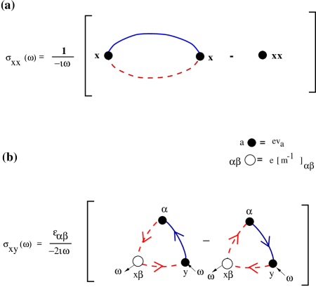
FIG. 8.: The diagrams contributing to (a) the conductivity and (b) the Hall conductivity in terms of Majorana fermions. (There are also a set of diagrams with the two Majorana parities interchanged.) In the electrical conductivity both species contribute equally in each diagram and the fast relaxation rate will dominate. By contrast, in the Hall conductivity there is an asymmetry between the number of each species of Majorana contributing to a given diagram. While the symmetry is restored by adding the diagrams with the parities interchanged, adding the diagrams is equivalent to adding conductivities and allows the long lived species to “short circuit” the rapidly decaying one in the Hall current.

C Derivation of the transport equation

The Boltzmann equation for charge conjugation eigenstates is determined from the semi-classical limit of the quantum Boltzmann equation. The derivation of the quantum Boltzmann equation (QBE) has been reviewed by Rammer and Smith [36] and we will rely heavily on their results. We proceed by deriving the QBE for electrons and their degenerate hole states as described by Rammer and Smith but, since our collision term will ultimately couple these two states, we group them together in a matrix. The perturbations that drive the Fermi system out of equilibrium—EM fields and temperature gradients etc—couple to electrons and holes directly and independently. Interactions in a conventional metal also preserve the electron or hole nature of the quasiparticles with the net result that the QBE is diagonal in the particle-hole basis and one solves for a single scalar distribution function. We wish to generalize this to the situation where the driving perturbations remain diagonal in the particle-hole basis but the interaction terms are diagonal only in the basis of charge conjugation eigenstates. To do this we will begin by deriving the driving terms in the QBE in the particle-hole basis by considering the collision-less system. We shall be careful though to make no assumption of commutivity since ultimately the collision term which we introduce will not be diagonal in this basis. Having obtained the driving terms we then rotate the equation into the basis of charge conjugation eigenstates where our phenomenological collision term is diagonal. This will then give our new transport equation from which we can obtain the conductivities.

The QBE is usually obtained from the equation of motion of the ‘Keldysh’ Green’s function. We therefore consider the time evolution of the following matrix Green’s function expressed in terms of particles and holes

$$\underline{G}^{K}(x_{1},{x_{1^{\prime}}}) \equiv G^{K}_{ij}(x_{1},x_{1^{\prime}})$$ (C1)

$$= -i\langle\left[\Psi^{\dagger}_{i}(x_{1}),\Psi_{j}(x_{1^{\prime}})\right]_{-}\rangle\;.$$ (C2)

Here $x_{1}$ is shorthand for the 4-coordinate $(t_{1},\vec{r}_{1})$. We deal first with the driving term in the QBE for which we need only consider the collision-less regime. Here the difference between the equation of motion acting on the left and right operators in $\underline{G}^{K}$ may be written as

$$\left[\delta(x_{1}-x_{1^{\prime}})\left(i\partial_{t_{1}}-\epsilon(-i\vec{\nabla}_{\vec{r}_{1}})\right)\underline{1}\stackrel{{\scriptstyle\otimes}}{{,}}\underline{G}^{K}\right]_{-}=\underline{0}\;,$$ (C3)

where $\otimes$ is the convolution operator in real space. This equation is now coarse grained in the presence of an EM field by introducing the mixed representation

$$\underline{G}(X,p)=\!\int\!\!dxe^{-i\vec{r}\cdot\left[\underline{\vec{p}}+e\vec{A}(X)\underline{1}\right]+it\left[E+e\varphi(X)\right]\underline{1}}\underline{G}(X,x),$$ (C4)

where $X$ is the center of mass coordinate $X=(x_{1}+x_{1^{\prime}})/2$ and we Fourier transform over the relative position $x=x_{1}-x_{1^{\prime}}$. To correctly transform the degenerate particle and hole states, the momentum $\underline{p}$ becomes a diagonal matrix

$$\underline{\vec{p}}=\left(\begin{array}[]{cc}\vec{p}&0\\ 0&-\vec{p}*\end{array}\right)\;.$$ (C5)

This transformation has the combined effect of coupling the system in a gauge invariant manner to the electro-magnetic field $A=(\varphi,\vec{A})$ and expressing everything in terms of the kinematic momentum. Under conditions of uniform, static electro-magnetic fields the convolution operator can be written in the mixed representation using the gradient expansion

$$G\otimes H=e^{{i\over 2}\left(\partial_{X}^{G}\cdot\partial_{p}^{H}-\partial_{p}^{G}\cdot\partial_{X}^{H}+\partial_{p}^{G}\cdot F\cdot\partial_{p}^{H}\right)}G(X,p)H(X,p)$$ (C6)

where $\partial_{p}^{G}$ denotes the derivative operator $(\partial_{E},\vec{\nabla})$ that acts exclusively on $G$ and $F$ is the usual antisymmetric EM field tensor $\partial_{\mu}A^{\nu}-\partial_{\nu}A^{\mu}$.

To obtain the classical limit of the QBE we simply apply the gradient expansion to first order to the equation of motion for $\underline{G}^{K}$. We now make the usual quasiparticle assumption [37, 38] that $\underline{G}^{K}$ is sharply peaked in energy $\sim\delta(\omega-\epsilon(\vec{k}))$ and we integrate the equation of motion over frequency. This leads then to the collision-less Boltzmann equation

$${1\over 2}\left\{\left(\begin{array}[]{c c}H_{\vec{p}}&0\\ 0&H_{\vec{p}*}\end{array}\right),\underline{G}^{K}(T,{\vec{R}},{\vec{p}})\right\}_{+}=\underline{0}\;,$$ (C7)

where, with $\vec{v}_{\vec{p}}=\vec{\nabla}_{\vec{p}}\epsilon(\vec{p})$, we define

$$H_{\vec{p}}=\partial_{T}+\vec{v}_{p}\cdot\vec{\nabla}_{\vec{R}}+e\left(\vec{E}+\vec{v}_{\vec{p}}\times\vec{B}\right)\cdot\vec{\nabla}_{\vec{p}}\;.$$ (C8)

We display the equations at this point to emphasis the fact that we have merely derived the conventional collision-less Boltzmann equation: the anticommutator here is trivial and we have two independent Boltzmann equations. However we now wish to express the above equation in terms of the charge conjugation eigenstates since our hypothesis for the scattering distinguishes between them. We apply the unitary transformation of Eq. B7 to rotate our transport equation into the basis of charge conjugation eigenstates

$$\underline{\dot{\rm f}}+{\textstyle{1\over 2}}\left\{\underline{\vec{\cal V}}_{{\rm\vec{p}}},\vec{\nabla}_{\rm R}\underline{\rm f}\right\}_{+}+{\textstyle{e\over 2}}\left\{(\vec{\rm E}+\underline{\vec{\cal V}}_{{\rm\vec{p}}}\times\vec{\rm B})\underline{\tau}_{2},\vec{\nabla}_{\rm p}\underline{\rm f}\right\}_{+}={\rm I}[\underline{g}]\;,$$ (C9)

where

$$\underline{\rm f}(T,\vec{R},\vec{p}) = \int d\omega\underline{U}^{-1}\underline{G}^{K}\underline{U}=\int d\omega\langle\left[\tilde{\Psi}^{\dagger}_{p}\tilde{\Psi}_{p}\right]_{-}\rangle,$$ (C10)

$$\;\underline{\vec{\cal V}}_{\vec{p}} = {1\over 2}\left(\vec{v}_{\vec{p}}+\vec{v}_{\vec{p}*}\right)\underline{1}+{1\over 2}\left(\vec{v}_{\vec{p}}-\vec{v}_{\vec{p}*}\right)\underline{\tau}_{2}\;.$$ (C11)

We have now added a collision integral, ${\rm I}[\underline{g}]$ which is a functional of the departure from equilibrium, $\underline{g}=\underline{\rm f}-\underline{\rm f}^{(0)}$. Our central hypothesis is now contained in this collision functional: the return to equilibrium is governed by two independent relaxation times—one for each of the charge conjugation eigenstates

$${\rm I}[\underline{g}]={1\over 2}\left\{\underline{\Gamma},\underline{g}\right\}_{+}={1\over 2}\left\{\left(\begin{array}[]{cc}\Gamma_{f}&0\\ 0&\Gamma_{s}\end{array}\right),\underline{g}\right\}_{+}$$ (C12)

Writing $\underline{\Gamma}=\Gamma_{+}\underline{1}+\Gamma_{-}\underline{\tau}_{3}$ we stress again that if $\Gamma_{-}=(\Gamma_{f}-\Gamma_{s})/2=0$ our transport equation is simply the usual relaxation time approximation used in text book treatments. The consequences of $\Gamma_{-}\neq 0$ are established in this paper.

REFERENCES

- [1] See for example, M. Gurvitch and A. T. Fiory, Phys. Rev. Lett. 59, 1337 (1987); L. Forro et al., ibid. 65, 1941 (1990).
- [2] T. R. Chien, Z. Z. Wang and N. P. Ong, Phys. Rev. Lett. 67, 2088 (1991).
- [3] P. W. Anderson, Phys. Rev. Lett. 67, 2092 (1991), see also Y. Ren and P. W. Anderson, Phys. Rev. B 48, 16662 (1993).
- [4] D. B. Romero, Phys. Rev. B 46, 8505 (1992).
- [5] An earlier summary of these ideas appeared in P. Coleman, A. J. Schofield and A. M. Tsvelik, Phys. Rev. Lett. 76, 1324 (1996); cond-mat/9602001.
- [6] J. M. Harris et al., Phys. Rev. Lett. 75, 1391 (1995).
- [7] N. P. Ong, Phys. Rev. B 43, 193 (1991).
- [8] J. Ziman, “Electrons and Phonons”, Oxford University Press, (1960). For a discussion of Kohler’s rule, see pp. 490. For a discussion of the Zener-Jones method see pp. 502.
- [9] I. Terasaki, Y. Sato, S. Miyamoto, S. Tajima and S. Tanaka, Phys. Rev. B 52, 16246 (1995).
- [10] T. Kimura , S. Miyasaka, H. Takagi et al., Phys. Rev. B 53, 8733 (1996).
- [11] S. G. Kaplan, S. Wu, H. T. S. Lihn and D. Drew, Q. Li, D. B. Fenner, Julia Phillips and S. Y. Hou, Phys. Rev. Lett. 76, 696 (1996).
- [12] H. D. Drew and P. Coleman, to be published (1996).
- [13] H. D. Drew, S. Wu and H-T. S. Lihn, proceedings of this conference.
- [14] A. Carrington, A. P. Mackenzie, C. T. Lin and J. R. Cooper, Phys. Rev. Lett. 69, 2855 (1992).
- [15] B. P. Stojkovic and D. Pines, Phys. Rev. Lett 76, 811 (1996); cond-mat/9505005.
- [16] R. Hlubina and T. M. Rice, Phys. Rev. B 51 9253, (1995); cond-mat/9501086.
- [17] B. G. Kotliar, A. Sengupta and C. M. Varma, Phys. Rev. B 53, 3573 (1996).
- [18] P. Voruganti, A. Golubentsev and S. John, Phys. Rev. B 45, 13945 (1992).
- [19] Superconducting fluctuations enhance the conductivity, but without changing the Hall conductivity, as shown recently by A. Aronov, S. Hikami and A. I. Larkin, Phys. Rev. B51, 3880 (1995). This means that the conductivity is enhanced, but the Hall angle is suppressed by superconducting fluctuations. By the f-sum and t-sum rules, this means that the decay rates of electric currents and Hall currents are reduced and enhanced respectively, by superconducting fluctuations.
- [20] Note that and are linked by the Onsager relation , where is the magnetic field.
- [21] see, for example, A. A. Abrikosov, Fundamentals of the Theory of Metals, North Holland, p. 103 (1988).
- [22] S. D. Obertelli, J. R. Cooper and J. L. Tallon, Phys. Rev. B, 46, 14928 (1992).
- [23] E. Majorana, Il Nuovo Cimento, 14, 171 (1937).
- [24] , since the Nernst Ettinghausen coefficient is negligible (): see J. A. Clayhold, A. W. Linnen Jr., F. Chien and C. W. Chu, Phys. Rev. B 50 4252, (1994).
- [25] with the leading temperature dependence coming from the thermal conductivity . The is phonon dominated: see C. Uher, in Physical properties of high temperature superconductors: vol. III p. 159, editor D. M. Ginsberg, World Scientific, Singapore (1992).
- [26] K. Krishana, J. M. Harris and N. P. Ong, Phys. Rev. Lett 75, 3529 (1995).
- [27] S. Brazovskii, Zh. Eksp. Teor Tiz. 68, 175 (1975); Sov. Phys. JETP 41, 85 (1975).
- [28] M. Gell-Mann and A. Pais, Phys. Rev. 97, 1387 (1955).
- [29] A. El Azruk, R. Nahoum, M. Guilloux-Viry, C. Thivet, A. Perrin, S. Labdi , Z. Z. Li and H. Raffy, Phys. Rev. B 49, 9846 (1994).
- [30] C. M. Varma, P. B. Littlewood, S. Schmitt-Rink, E. Abrahams and A. E. Ruckenstein, Phys. Rev. Lett., 63 1996, (1989).
- [31] A. E. Ruckenstein and C. M. Varma, Physica C, 185-189, 134, (1991).
- [32] P. Coleman, L. Ioffe and A. M. Tsvelik, Phys. Rev. B 52, 6611 (1995); cond-mat/9504006.
- [33] P. Coleman, E. Miranda and A. M. Tsvelik, Phys. Rev. Lett. 74, 1653 (1995); cond-mat/9406085.
- [34] E. Abrahams, A. Balatsky, D. J. Scalapino and J. R. Schrieffer, Phys. Rev. B, 52, 1271 (1995); cond-mat/9503071.
- [35] Note that by choosing so that electrons and holes are degenerate to quadratic order, we will ensure that this Hamiltonian is diagonal to quadratic order. For the calculations we describe, an explicit form for the quadratic corrections to is not required.
- [36] J. Rammer and H. Smith, Rev. Mod. Phys. 58, 323 (1986).
- [37] One might argue that a scattering rate is in contradiction to the assumption of a well defined quasi-particle peak in the spectral function. Under these circumstances one can integrate over momentum as is done for the high temperature electron-phonon systems to derive a similar transport equation.
- [38] L. P. Kadanoff and G. Baym, Quantum statistical mechanics, W. A. Benjamin, New York (1962).