Can Hall drag be observed in Coulomb coupled quantum wells in a magnetic field?

Abstract

We study the transresistivity $\tensor{\rho}_{21}$ (or equivalently, the drag rate) of two Coulomb-coupled quantum wells in the presence of a perpendicular magnetic field, using semi-classical transport theory. Elementary arguments seem to preclude any possibility of observation of “Hall drag” (i.e., a non-zero off-diagonal component in $\tensor{\rho}_{21}$). We show that these arguments are specious, and in fact Hall drag can be observed at sufficiently high temperatures when the intralayer transport time $\tau$ has significant energy-dependence around the Fermi energy $\varepsilon_{F}$. The ratio of the Hall to longitudinal transresistivities goes as $T^{2}Bs$, where $T$ is the temperature, $B$ is the magnetic field, and $s=[\partial\tau/\partial\varepsilon](\varepsilon_{F})$.

I Introduction

When two quantum wells are placed sufficiently close together (but far enough apart so inter-well tunneling is negligible), Pogrebinskii and Price[1] predicted that the interlayer electron–electron ($e$–$e$) interactions would be enough so that a drift of carriers in one layer causes a discernable drag in the other. Such a “Coulomb drag” effect has been measured[2] using in a set-up shown schematically Fig. 1, and its observation has prompted a barrage of theoretical studies[3, 4, 5, 6, 7, 8].

Experimentalists are now extending their studies to Coulomb drag in systems with a magnetic field $B$ perpendicular to the layers[9]. Present efforts are mainly focussed on the high $B$-field regime, when Landau levels are fully resolved, and interesting effects from the quantization have been predicted[8]. In this regime, the drag electric field response ${\bf E}_{2}$ was shown using the Kubo formalism to be parallel to the driving current ${\bf J}_{1}$ (to lowest non-vanishing order in the interlayer interaction and $1/B$). The question naturally arises: are there circumstances when one can find ${\bf E}_{2}$ with a component perpendicular to ${\bf J}_{1}$; i.e., Hall drag? And if so, what does this tell us about the system?

In this paper, we first present a seemingly plausible explanation for why, at the level of the Born approximation, Hall drag cannot exist. We then reveal the flaw behind the explanation and show that Hall drag is possible in principle. Using a low temperature ($T$) expansion, we show that the Hall transresistivity should go as $T^{4}$, and that the magnitude of the Hall drag gives information on the energy-dependence of the intralayer transport time at the Fermi surface. We argue that, for certain systems, one should be able to see Hall drag at intermediate magnetic fields and high enough temperatures.

II Fallacious argument against Hall drag

As mentioned previously, the quantity which is usually measured experimentally is the transresistivity $\tensor{\rho}_{21}$, defined by

$$\tensor{\rho}_{21}{\bf J}_{1}={\bf E}_{2},$$ (1)

with ${\bf J}_{2}=0$. In the absence of a magnetic field in an isotropic system, symmetry clearly dictates that ${\bf E}_{2}$ and ${\bf J}_{1}$ must be parallel to each other. When a symmetry-breaking perpendicular $B$-field is imposed system, is it then possible to observe “Hall drag” voltage; i.e. a nonzero off-diagonal element in $\tensor{\rho}_{21}$?

From a macroscopic point of view, the following simple argument seems to preclude the existence of Hall drag (barring quantum correlation effects which go beyond the Born approximation utilized in this paper). In a drag experiment, the drive current ${\bf J}_{1}$ produces a parallel force ${\bf F}_{21}$ on the carriers in layer 2. In steady state, the total net force on carriers in layer 2 must be zero. The additional forces acting on these carriers are the induced electric field, $e_{2}{\bf E}_{2}$ ($e_{i}$ is the charge in layer $i$), forces due to the imposed magnetic field ${\bf J}_{2}\times{\bf B}$ and the lattice scattering. Since ${\bf J}_{2}=0$, both the Lorentz force and lattice scattering are zero. Therefore, $e_{2}{\bf E}_{2}={\bf F}_{21}$, and since ${\bf F}_{21}|\!|{\bf J}_{1}$, ${\bf J}_{1}$ must also be parallel to ${\bf E}_{2}$. That is, there should be no Hall drag.

This argument in specious on two counts. First, ${\bf F}_{21}$ need not be parallel to ${\bf J}_{1}$. The ${\bf F}_{21}$ depends on the exact nature of the distribution function $f_{1}({\bf k})$ of layer 1 in the presence of the driving electric field. When symmetry is broken by application of a magnetic field, $f_{1}({\bf k})$ may become skewed in a manner which results in non-parallel ${\bf F}_{21}$ and ${\bf J}_{1}$. Second, even though ${\bf J}_{2}=0$, the carriers in layer 2 are not in equilibrium, because they are continuously being acted upon by the drag force and induced electric field ${\bf E}_{2}$. Therefore, since $f_{2}({\bf k})$ is not necessarily equal to the equilibrium distribution function, it is possible for the lattice to exert a net force on the carriers in spite of the absence of a net current.

Thus, the presence or absence of measurable Hall drag in a Coulomb coupled system depends crucially on the microscopic details of the system. In particular, as we show below, Hall drag depends on the energy dependence of the intralayer scattering mechanisms around the Fermi surface. In this way, Hall drag measurements are distinct from the usual transport single layer Hall measurements, which are generally quite insensitive to the details of the energy-dependence of the scattering mechanisms.

III Formalism

In this paper, we only treat cases where the $B$-field is small enough that Landau quantization is not significant (i.e., the cyclotron frequency is much less than the inverse lifetime of the electrons), and the interlayer interaction $W_{21}$ is weak so that one can work to the lowest non-vanishing (second) order in $W_{21}$; i.e., in the Born approximation. Given these assumptions, the semi-classical Boltzmann equation description is a valid description of the system. We also assume that the carriers in an isotropic parabolic band with effective mass $m_{i}^{*}$.

The semi-classical theory gives the transconductivity $\tensor{\sigma}_{21}$ from which the transresistivity is obtained by

$$\tensor{\rho}_{21}=-\tensor{\rho}_{22}\tensor{\sigma}_{21}\tensor{\rho}_{11}$$ (2)

where $\tensor{\rho}_{ii}$ are the resistivity tensors of the individual layers. Following the formalism in Ref. [7], generalized to include a $B$-field in the $z$-direction, the transconductivity is given by

$$\tensor{\sigma}_{21}({\bf B})=\frac{e_{1}e_{2}}{8\pi k_{B}T}\int\frac{d{\bf q}}{(2\pi)^{2}}\int_{0}^{\infty}d\omega\ \frac{|W_{21}({\bf q},\omega)|^{2}}{\sinh^{2}(\hbar\omega/2k_{B}T)}$$ (3)

$$\ {\bf\Delta}_{2}({\bf q},\omega;-{\bf B})\ {\bf\Delta}_{1}({\bf q},\omega;{\bf B}).$$ (4)

The interlayer coupling $W_{21}$ is the screened Coulomb interaction evaluated within the Thomas-Fermi approximation.

In the Kubo formalism, ${\bf\Delta}$ is given diagrammatically by three Green functions arranged in a triangle[5, 6]. In the Boltzmann formalism, ${\bf\Delta}$ is related to the linear response in the distribution functions $f_{i}({\bf k})$ of the individual electron gases $i$ to a small uniform perturbing electric field. Let ${\bf\Psi}_{{\bf B},i}({\bf k})$ be the quantity which describes the perturbation to $f_{i}({\bf k})$ which would result from the application of a small electric field ${\bf E}_{i}$, in the presence of magnetic field B,

$$\delta f_{i}({\bf k})\equiv f_{i}({\bf k})-f^{0}_{i}({\bf k})=f^{0}_{i}({\bf k})\,(1-f^{0}_{i}({\bf k}))\;e_{i}{\bf E}_{i}\cdot{\bf\Psi}_{{\bf B},i}({\bf k}),$$ (5)

where $f^{0}_{i}({\bf k})$ is the equilibrium Fermi-Dirac distribution function of layer $i$. It can be shown that[10]

$${\bf\Delta}_{i}({\bf q},\omega;{\bf B}) \equiv 4\pi k_{B}T\int\frac{d{\bf k}_{i}}{(2\pi)^{2}}\ [{\bf\Psi}_{{\bf B},i}({\bf k}_{i}+{\bf q})-{\bf\Psi}_{{\bf B},i}({\bf k}_{i})]$$ (7)

$$[f_{i}^{0}({\bf k}_{i})-f_{i}^{0}({\bf k}_{i}+{\bf q})]\ \delta(\varepsilon_{\bf k_{i}}-\varepsilon_{\bf k_{i}+q}-\hbar\omega),$$

Furthermore, the single layer conductivities are also related to ${\bf\Psi}$ by[10]

$$\tensor{\sigma}_{ii}({\bf B})=2e_{i}^{2}k_{B}T\int\frac{d{\bf k}}{(2\pi)^{2}}\ \left(-{f^{0}_{i}}^{\prime}(\varepsilon)\right)\,{\bf v}_{{\bf k},i}\,\Psi_{{\bf B},i}({\bf k})$$ (8)

and $\tensor{\rho}_{ii}$ can be obtained by inverting $\tensor{\sigma}_{ii}$.

A $\Psi$ in a $B$-field

We assume the intralayer scattering of the system dominated by elastic (e.g., impurity) and quasi-elastic (e.g., acoustic phonon) scattering, as is the case for GaAs under 40 K. Under these circumstances, the scattering can be described by an energy-dependent transport time $\tau(\varepsilon)$, whose exact functional form of course depends on the particular system being studied. Then, ${\bf\Psi}_{{\bf B},i}$ is[11]

$${\bf\Psi_{{\bf B},i}(k)} = \frac{\tau_{i}(\varepsilon_{k})}{k_{B}T}\frac{{\bf v}_{{\bf k},i}-{\bf v}_{{\bf k},i}\times\hat{\bf z}\,(\omega_{c,i}\tau_{i}(\varepsilon_{k}))}{1+(\omega_{c,i}\tau_{i}(\varepsilon_{k}))^{2}},$$ (9)

$$= \frac{\tau_{i}(\varepsilon_{k})v_{k}}{k_{B}T\sqrt{1+(\omega_{c}\tau_{i}(\varepsilon_{k}))^{2}}}\ \hat{\bf a}_{i}(\varepsilon_{k})$$ (10)

where ${\bf v}_{\bf k}$ is the velocity, $\omega_{c,i}=e_{i}B/m^{*}_{i}$ is the cyclotron frequency and $\hat{\bf a}$ is a unit vector rotated at an angle $-\tan^{-1}(\omega_{c,i}\tau(\varepsilon_{k}))$ from ${\bf k}$. This is shown schematically in Fig. 2.

B Energy-independent $\tau_{i}$

In the case when the $\tau_{1}$ is energy-independent, $\hat{\bf a}_{1}$ is a constant. Then, Eq. (10) shows that $\delta f_{1}$ is inversion symmetric with respect to $\hat{\bf a}_{1}$, which implies that the current ${\bf J}_{1}$ is parallel to ${\bf a}_{1}$ and, from the Born approximation expression for the force transferred from layer 1 to 2[4], that ${\bf F}_{21}$ is parallel to ${\bf J}_{1}$. Furthermore, the net lattice force on carriers in layer 2 for energy-independent $\tau_{2}$ is simply proportional to ${\bf J}_{2}$, and hence is zero in a transresistivity experiment. Thus, in this special case, the specious arguments given in Sec. II actually hold, and there is no Hall drag.

C Energy-dependent $\tau_{i}$

However, the sophistry of the argument is exposed once $\tau_{i}$ is energy-dependent. The energy dependence of $\hat{\bf a}_{1}$ then results in a $\delta f_{1}$ which is no longer inversion symmetric with respect to the axis of ${\bf J}_{1}$, and consequently ${\bf F}_{21}$ is not necessarily parallel to ${\bf J}_{1}$. Furthermore, the lattice can exert a non-zero force on the carriers in layer 2 (despite ${\bf J}_{2}$ being zero) which is non-parallel to ${\bf F}_{21}$. Thus, in principle Hall drag can exist.

IV Magnitude of Hall drag: small $T$ expansion

Merely giving an existence argument is insufficient; one would like to know if the effect is experimentally observable. We address this point in this section, by calculating the low temperature behavior of $\tensor{\rho}_{21}^{xy}$.

We first linearise the energy-dependence of the transport time about the Fermi energy $\varepsilon_{F}$,

$$\tau(\varepsilon)=\tau_{0}\left(1+s\frac{\xi}{\varepsilon_{F}}\right),$$ (11)

$\xi=\varepsilon-\varepsilon_{F}.$ We also find it convenient to write the conductivity and resistivity tensors in terms of a product of a scalar and rotation matrix

$$\hat{R}(\theta)=\left(\matrix{\cos\theta&-\sin\theta\cr\sin\theta&\cos\theta}\right)$$ (12)

which rotates vectors clockwise by angle $\theta$. The magnitude and rotation angle of $\tensor{\rho}$ ($\tensor{\sigma}$) are denoted by $\varrho$ ($\varsigma$) and $\theta$ ($\phi$), respectively; i.e.,

$$\tensor{\rho}_{ij}(B,T) = \varrho_{ij}(B,T)\;\hat{R}\Bigl{(}\theta_{ij}(B,T)\Bigr{)};$$ (13)

$$\tensor{\sigma}_{21}(B,T) = \varsigma_{ij}(B,T)\;\hat{R}\Bigl{(}\phi_{ij}(B,T)\Bigr{)}.$$ (14)

Therefore, from Eq. (2),

$$\varrho_{21} = -\varrho_{22}\,\varsigma_{21}\,\varrho_{11};$$ (15)

$$\theta_{21} = \theta_{22}+\phi_{21}+\theta_{11}.$$ (16)

We denote the $n$-th coefficient of an expansion in powers of $T$ of quantity $A$ as $A^{(n)}$; e.g.,

$$\theta_{ij}(B,T) = \sum_{n=0}^{\infty}\theta_{ij}^{(n)}(B)\;T^{n}.$$ (17)

A The $T\rightarrow 0$ limit

First, let us briefly review some results of Coulomb drag in the absence of a $B$-field. At $B=0$, all the rotation angles in an isotropic system are clearly zero by symmetry. Due to phase space considerations, in the low temperature limit[12] $\sigma_{21}(B=0,T)=\varsigma_{21}^{(2)}(0)T^{2}+O(T^{3})$, as in $e$–$e$ scattering in a single two-dimensional layer [13]. Since $\varrho_{ii}^{(0)}(B=0)=m^{*}_{i}/(n_{i}e_{i}^{2}\tau_{0,i})$ ($n_{i}$ is the density), Eq. (2) implies that $\rho_{21}(B=0,T)$ also has a quadratic temperature dependence. The leading order coefficients $\varrho_{21}^{(2)}(B=0)$ and $\varsigma_{21}^{(0)}(B=0)$ are given elsewhere[4, 7].

In the presence of a magnetic field, Eqs. (4) and (8), together with Eqs. (7) and (10), yield to lowest non-vanishing order in $T$

$$\varrho_{ii}^{(0)}(B) = \varrho_{ii}^{(0)}(B=0)\left(1+\Omega_{c,i}^{2}\right)^{1/2}$$ (18)

$$\varsigma_{21}^{(2)}(B) = \frac{\varsigma_{21}^{(2)}(B=0)}{[(1+\Omega_{c,1}^{2})(1+\Omega_{c,2}^{2})]^{1/2}}$$ (19)

$$\theta_{ii}^{(0)}(B) = \tan^{-1}(\Omega_{c,i});$$ (20)

$$\phi_{21}^{(0)}(B) = -\tan^{-1}(\Omega_{c,1})-\tan^{-1}(\Omega_{c,2}),$$ (21)

where $\Omega_{c,i}=\omega_{c,i}\tau_{0,i}$. From Eqs. (15), (16) and (18) – (21), we obtain $\theta_{\rho,21}^{(0)}(B)=0$ and

$$\varrho_{21}^{(2)}(B) = \varrho_{21}^{(2)}(B=0).$$ (22)

This means that $\tensor{\rho}_{21}(B,T\rightarrow 0)$ is independent of the magnetic field, and hence the ratio of the Hall to normal drag coefficients in this limit is

$$\lim_{T\rightarrow 0}\ \frac{\rho^{xy}_{21}(B,T)}{\rho^{xx}_{21}(B,T)}=0.$$ (23)

The fact that the Hall drag disappears faster than normal drag as $T\rightarrow 0$ is a consequence of the lack of symmetry-breaking in the distribution function in this limit. From Eq. (5), one sees that $\delta f_{i}({\bf k})$ is significant only around an energy of order of a few $k_{B}T$ about the Fermi energy. If the scattering time $\tau_{i}(\varepsilon)$ does not change significantly within this energy range, then the symmetry breaking in $\delta f_{i}$ will be small, and consequently so will the Hall drag effect. One needs to go to larger temperature to see a measurable Hall drag signal.

To obtain the first non-vanishing term in the $T$-expansion of $\rho_{21}^{xy}$, we expand the rotation angles $\theta_{ii}$ and $\phi_{21}$ in powers of $T$. This is achieved by expanding $\Psi$ in powers of $\xi$, and using this expansion in Eq. (8). Inverting $\tensor{\sigma}_{ii}$, we find $\theta_{ii}^{(1)}=0$ and

$$\theta_{ii}^{(2)} = \frac{\pi^{2}s_{i}\Omega_{c,i}(1+s_{i}+\Omega_{c,i}^{2}-s_{i}\Omega_{c,i}^{2})}{3(1+\Omega_{c,i}^{2})^{2}}\;\frac{k_{B}^{2}}{\varepsilon_{F,i}^{2}}.$$ (24)

The angle $\theta_{ii}$ increases with increasing $s$ (for $\Omega_{c,i}^{2}<1$) because the particles with larger velocities, which contribute more to the overall conductivity, have a larger deflection with respect to ${\bf E}_{i}$ (see Eq. (10)).

At this point to simplify the algebra (which otherwise would be daunting), it is henceforth assumed that both the layers are identical, and therefore the layer indices for all the parameters shall be dropped. We also assume that the well widths $L$ are zero, and the inter-well spacing $d$, the Fermi wavevector $k_{F}$ and the the Thomas-Fermi screening length $q_{\rm TF}$ satisfy the conditions $(k_{F}d)^{-1}\ll 1$ and $(q_{\rm TF}d)^{-1}\ll 1$. Hence, the results presented here are only valid to lowest order in these quantities.

Expanding ${\bf\Delta}$ in powers of $\omega$ in Eq. (4) yields $\phi_{21}^{(1)}(B)=0$ and

$$\phi_{21}^{(2)}(B) = \frac{\pi^{2}s\Omega_{c}(1-2s+\Omega_{c}^{2}+2s\Omega_{c}^{2})}{3(1+\Omega_{c}^{2})^{2}}\;\frac{k_{B}^{2}}{\varepsilon_{F}^{2}}$$ (25)

From Eqs. (16), (24) and (25), the small $T$ rotation angle of $\tensor{\rho}_{21}$ is

$$\theta_{21}(T)\approx\frac{\pi^{2}s\Omega_{c}}{(1+\Omega_{c}^{2})}\;\frac{(k_{B}T)^{2}}{\varepsilon_{F}^{2}}.$$ (26)

For small angles, $\sin\theta\approx\theta$, and hence that the ratio of the Hall to longitudinal transresistivities is coefficient is

$$\frac{\rho_{21}^{xy}(B,T)}{\rho_{21}^{xx}(B,T)}=\frac{\pi^{2}s\Omega_{c}}{(1+\Omega_{c}^{2})}\;\frac{(k_{B}T)^{2}}{\varepsilon_{F}^{2}}+O(T^{3})$$ (27)

Since $\rho_{21}^{xx}\propto T^{2}$, this shows that $\rho_{21}^{xy}\propto T^{4}$.

For positive $s$ and like charges in layers 1 and 2, both $\theta_{11}$ and $\theta_{21}$ have the same sign. Since $\varrho_{ii}^{(0)}$ and $\varsigma_{ii}^{(2)}$ (for like charges) are positive, the negative sign in Eq. (15) means that the Hall fields in the driving and drag layer are in opposite directions. From an experimental point of view, this is favourable because a Hall drag signal cannot be mistaken for a leakage voltage from the driving layer[14].

V Discussion

Since the magnitude of $\rho_{21}^{xy}$ is proportional to $s$, one would like to have a large value of $s$ to obtain an experimentally clear signal. Herein lies a problem. Generally in the modulation doped samples currently used in drag experiments, the remote dopants are placed far away in order to obtain high mobilities in the quantum wells. This means that the intralayer $e$–$e$ scattering is much stronger than either the impurity scattering or acoustic phonon scattering, and hence even when the system is driven by external forces, the $f({\bf k})$ tends to relax towards a drifted Fermi-Dirac distribution. A drifted Fermi-Dirac distribution function is equivalent to a ${\bf\Psi}$ in Eq. (10) with a constant $\tau$; i.e., with $s=0$. Therefore, when intralayer $e$–$e$ scattering dominates, Hall drag will be difficult to measure.

To get a measurable Hall drag signal, one needs to increase $s$. This can be done by putting the charged dopants close to the quantum wells. As shown in Ref. [15], when the dopants are placed on the order of $150\;{\rm\AA}$ from the side of a GaAs well doped to $1.5\times 10^{11}\,{\rm cm}^{-2}$, one can achieve an $s$ on the order of 0.4. The factor $\Omega_{c}/(1+\Omega_{c}^{2})$ has a maximum of 1/2 at $\Omega_{c}=1$[16], and therefore the prefactor in Eq. (27), $\pi^{2}s\Omega_{c}/(1+\Omega_{c}^{2})$ can be made larger than one, which should facilitate measurement of Hall drag.

To conclude, we have shown that it is possible to measure Hall drag in Coulomb coupled quantum wells. The Hall drag coefficient $\rho_{21}^{xy}$ goes as $T^{4}$, and it probes the $\varepsilon$ dependence of the transport time $\tau(\varepsilon)$ in the vicinity of the Fermi energy. Note that the single layer Hall coefficient also depends to some extent on the $\varepsilon$ dependence of $\tau(\varepsilon)$ through the Hall coefficient[17] $r_{H}=\langle\tau^{2}(\varepsilon)\rangle/\langle\tau(\varepsilon)\rangle^{2}$ (where $\langle\cdots\rangle$ denotes thermal averaging). However, the $\varepsilon$-dependence in $\tau(\varepsilon)$ gives a correction factor to $r_{H}$, whereas it affects Hall drag to leading order, and therefore Hall drag is a much more sensitive probe of $\tau(\varepsilon)$.

VI Acknowledgement

We thank Martin Christian Bønsager and Karsten Flensberg for useful discussions.

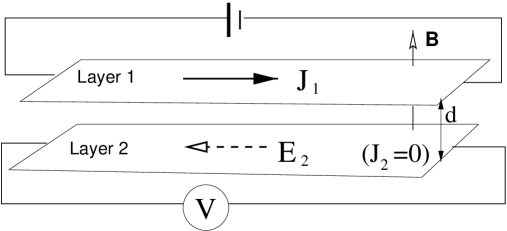
FIG. 1.: Schematic diagram of drag experiment. Two independently contacted two-dimensional electron gases are placed close together. A current ${\bf J}_{1}$ is driven through layer 1, and layer 2 is connected to a voltmeter (so that ${\bf J}_{2}=0$). The interlayer $e$–$e$ interactions cause a drag response electric field ${\bf E}_{2}$ in layer 2. If a magnetic field ${\bf B}$ perpendicular to both layers is applied, can ${\bf E}_{2}$ have a component perpendicular to ${\bf J}_{1}$? We show that this should be possible for high enough temperatures and large enough energy dependence of intralayer transport times.

FIG. 2.: Schematic contour plot of distribution function of carriers in the ${\bf k}$-plane, in an applied magnetic field for non-constant $\tau(\varepsilon)$. The dotted and solid lines are for carriers in equilibrium and in an electric field ${\bf E}$, respectively. When ${\bf E}$ is applied, the contours shift in different directions, as shown by the small arrows, due to the variation $\tau(\varepsilon)$ [see Eq. (10)]. The resultant net current is ${\bf J}$.

REFERENCES

- [1] Pogrebinskii, M. B., Fiz. Tekh. Poluprovodn. 11, 637 (1977) [Sov. Phys. Semicond. 11, 372 (1977)]; Price, P. J., Physica B 117 750 (1983).
- [2] Solomon, P. M., Price, P. J., Frank, D. J. and La Tulipe, D. C., Phys. Rev. Lett. 63, 2508 (1989); Gramila, T. J., Eisenstein, J. P., MacDonald, A. H., Pfeiffer, L. N. and West, K. W., Phys. Rev. Lett. 66, 1216 (1991); Phys. Rev. B 47, 12957 (1993); Physica B 197, 442 (1994); Sivan, U., Solomon P. M. and Shtrikman, H., Phys. Rev. Lett. 68, 1196 (1992).
- [3] Laikhtman, B., and Solomon, P. M., Phys. Rev. B 41, 9921 (1990); Boiko, I. I. and Sirenko, Yu. M., Phys. Stat. Sol. 159, 805 (1990); Solomon, P. M. and Laikhtman, B., Superlatt. Microstruct. 10, 89 (1991); Rojo, A. G. and Mahan, G. D., Phys. Rev. Lett. 68, 2074 (1992); Tso, H. C., Vasilopoulos, P. and Peeters, F. M., Phys. Rev. Lett. 68, 2516 (1992), Phys. Rev. Lett. 70, 2146 (1993); Tso, H. C. and Vasilopoulos, P., Phys. Rev. B 45, 1333 (1992); Maslov, D. I., Phys. Rev. B 45, 1911 (1992); Duan, J.-M. and Yip, S., Phys. Rev. Lett. 70, 3647 (1993); Zheng, L. and MacDonald, A. H., Phys. Rev. B 48, 8203 (1993); Cui, H. L., Lei, X. L. and Horing, N. J. M., Superlatt. Microstruct. 13, 221 (1993); Shimshoni, E. and Sondhi, S. L., Phys. Rev. B 49, 11 484 (1994); Flensberg, K. and Hu, B. Y.-K., Phys. Rev. Lett. 73, 3572 (1994); Świekowski, L., Szymański, J. and Gortel, Z. W., Phys. Rev. Lett. 74, 3245 (1995); Duan, J.-M., Europhys. Lett. 29, 489 (1995); Vignale, G. and MacDonald, A. H., Phys. Rev. Lett. 76, 2789 (1996); Wu, M. W., Cui, H. L. and Horing, N. J. M., Report No. cond-mat/9604004 (to be published in Mod. Phys. Lett. B).
- [4] Jauho, A.-P. and Smith, H., Phys. Rev. B 47, 4420 (1993).
- [5] Kamenev, A. and Oreg, Y., Phys. Rev. B 52, 7516 (1995).
- [6] Flensberg, K., Hu, B. Y.-K., Jauho, A.-P., and Kinaret, J., Phys. Rev. B 52, 14761 (1995).
- [7] Flensberg, K. and Hu, B. Y.-K., Phys. Rev. B 52, 14796 (1995).
- [8] Bønsager, M. C., Flensberg, K., Hu, B. Y.-K. and Jauho, A.-P., to be published in Phys. Rev. Lett.
- [9] Eisenstein, J. P.; Gramilla, T. J.; Hill, N. (private communication).
- [10] Hu, B. Y.-K. and Flensberg, K. (unpublished).
- [11] See e.g. Askerov, B. M., “Electron Transport Phenomena in Semiconductors” (World Scientific, Singapore, 1994); p. 105 – 106.
- [12] We ignore diffusion effects which result in a logarithmic correction to the temperature dependence, as shown in Zheng, L. and MacDonald, A. H., Phys. Rev. B 48, 8203 (1993).
- [13] Hodges, C., Smith, H. and Wilkins, J. W., Phys. Rev. B 4, 302 (1971); Giuliani, G. F. and Quinn, J. J., Phy. Rev. B 26, 4421 (1982).
- [14] Gramila, T. J. (private communication).
- [15] Hu, B. Y.-K. and Flensberg, K., Phys. Rev. B 53, 10072 (1996).
- [16] Note that the transport time can be an order of magnitude larger than the lifetime [see Das Sarma, S. and Stern, F., Phys. Rev. B 32 8442 (1985)], so semiclassical theory is valid even when .
- [17] See e.g., Seeger, K., “Semiconductor Physics” (Springer, Berlin, 1985), 3rd. Ed., p. 57.