[

Intermediate-Coupling Theory for the Spectral Weight of Spin Polaron

Abstract

Within the intermediate-coupling theory, the quasiparticle weight $Z$ of one hole injected in the undoped antiferromagnetic ground state is studied. We find that, for the hole located at the quasiparticle band minimun with momentum ${\bf k}_{0}=(\pm\frac{\pi}{2},\pm\frac{\pi}{2})$, $Z$ is finite. By comparing the results obtained by the self-consistent Born approximation, we show that the intermediate-coupling theory for $Z$ is appropriate only when $J/t\stackrel{{\scriptstyle>}}{{\sim}}1.6$. Finally, the reason why this approach fails in the small-$J$ case will also be clarified.

]

The problem for the motion of a hole in a 2D antiferromagnet (AF) has received significant attention [1] especially since the discovery of the copper oxide superconductors, where superconductivity arises from the doping of holes in an antiferromagnetic insulator. The AF with one hole is also a highly non-trivial correlated electronic system, and is therefore of fundamental interest from a theoretical point of view.

Intuitively one would expect that the presence of a hole in an AF leads to a distortion of the underlying spin configuration, in a similar way as a conduction electron in a polar crystal causes a deformation of the lattice. Indeed, under the assumptions that the AF is not completely destroied by doping a hole and that the low-energy excitations of the spin background are spin waves, one arrives at the following effective Hamiltonian [2, 3], $\tilde{H}$, which is reminiscent of Fröhlich’s polaron Hamiltonian [4] :

$$\tilde{H} = H_{t}+H_{J},$$ (1)

$$H_{J} = \sum_{\bf q}\omega_{\bf q}b_{\bf q}^{\dagger}b_{\bf q},$$ (2)

$$H_{t} = \frac{\alpha\omega}{\sqrt{N}}\sum_{\bf k,q}(M_{\bf q}({\bf k})f_{\bf k-q}^{\dagger}f_{\bf k}b_{\bf q}^{\dagger}+h.c.)$$ (3)

Here $b_{\bf q}$ and $f_{\bf k}$ are the annihilation operators of the hole and the spin wave. $\omega_{\bf q}=\omega\nu_{\bf q}$ is the spin wave excitation spectrum, where $\omega=Jz/2$, $\nu_{\bf q}=\sqrt{1-\gamma_{\bf q}^{2}}$, and $\gamma_{\bf q}=\sum_{\bf d}e^{i{\bf q\cdot d}}/z$ with ${\bf d}$ the unit vectors to nearest neighbors and $z$ being the coordination number ( $z=4$ for a 2D square lattice ). $\alpha=2t/J$ is the dimensionless coupling parameter ( therefore, the small-$J$ limit means the strong-coupling limit of $\tilde{H}$ ), $N$ is the number of the lattice sites, and $M_{\bf q}({\bf k})=\hbox{cosh}\theta_{\bf q}\gamma_{\bf k-q}+\hbox{sinh}\theta_{\bf q}\gamma_{\bf k}$ is the coupling function between the hole and the spin wave, where $\hbox{cosh}\theta_{\bf q}=[(1+\nu_{\bf q})/(2\nu_{\bf q})]^{1/2}$ and $\hbox{sinh}\theta_{\bf q}=-{\rm sgn}(\gamma_{\bf q})[(1-\nu_{\bf q})/(2\nu_{\bf q})]^{1/2}$ are the Bogoliubov transformation coefficients. Based on this similarity [5], a hole in an AF may be viewed as a “ spin polaron ”, i.e., a hole dressed by a cloud of virtual spin-wave excitations of the antiferromagnetic spin background. From this observation, the intermediate-coupling treatment [6] of the Fröhlich polaron problem is recently applied to the present spin-polaron problem by Barentzen [7]. It is found that : (1) the intermediate-coupling results for the quasi-particle energy $E(\bf k)$ is in agreement with the dispersion curve obtained by means of a Green function Monte Carlo method [8]; (2) the result for the bandwidth $W$ is quite good for weak coupling ( $J/t>3$ ), and is still reasonably good in the intermediate range ( $0.4\stackrel{{\scriptstyle<}}{{\sim}}J/t\leq 3$ ), where the deviation from the values obtained by the self-consistent Born approximation ( SCBA ) [9] was about 10 - 20 %. Thus the intermediate-coupling theory may be appropriate for $J/t\stackrel{{\scriptstyle>}}{{\sim}}0.4$.

One of the most controversial issues in the spin-polaron problem is whether a hole injected in the undoped ground state behaves like a quasiparticle [10], or, equivalently, whether the quasiparticle weight ( or the wavefunction renormalization constant ) $Z$ at the Fermi surface is finite under the dressing by the spin-wave excitations. There have already been many studies along this line (see [1] for further references). However, most of the previous studies have involved numerical calculations on small clusters ( even the studies using the SCBA have to solve Dyson’s equation numerically for small clusters ). Although numerical calculations on clusters show that the hole has a finite quasiparticle weight, there is still some uncertainty as to whether the quasiparticle weight vanishes or not in the thermodynamic limit [11].

In this report, we will study the quasiparticle weight within the intermediate-coupling theory, in which we can freely take the thermodynamic limit. Since, when a single hole is doped, the hole will locate at the quasiparticle band minimun with momentum ${\bf k}_{0}=(\pm\frac{\pi}{2},\pm\frac{\pi}{2})$ [1], we will confine ourselves to the spectral weight of the hole at momentum ${\bf k}_{0}$. We find that the deviation from the results of Refs. [9] is below 20 % only when $J/t\stackrel{{\scriptstyle>}}{{\sim}}1.6$. Thus the range of validity for $Z$ is smaller than that for $W$. Moreover, we will point out that, although this approach is not plagued with the finite-size effect, due to its mean-field nature, the infrared behavior of the present system may not be correctly described by this method even qualitatively ! This may be the reason why the intermediate-coupling theory for the spin-polaron problem is not as successful as that for the lattice-polaron case.

In order to compare with the results obtained by SCBA [9], rather than starting from the Hamiltonian used in Barentzen’s paper ( Eq.(11) of Ref. [7], which is denoted as $H_{Bar}$ in the present report ), we take Eq.(2) as our starting point, where the Bogoliubov transformation has been taken, such that the unperturbated ground state is the vacuum state for the spinless fermion operators and the quantum Néel state, $|0\rangle$, with respect to the spin-wave operators $b_{\bf q}$. The relation between $\tilde{H}$ and $H_{Bar}$ is simply

$$\tilde{H}=V^{\dagger}H_{Bar}V,$$ (4)

where $V$ denotes the unitary operator of the Bogoliubov transformation.

Following the procedure in Ref. [7], one first makes a change of coordinates to the rest frame of the moving hole by the unitary operator ( i.e., the so-called Jost transformation ) [12]

$$U=\sum_{\bf k,p}(\frac{1}{N}\sum_{i}T_{i}e^{-i{\bf p}\cdot{\bf R}_{i}})f_{\bf k}^{\dagger}f_{\bf k-p},$$ (5)

where the translation operators for the bosons are defined by

$$T_{i}=\hbox{exp}(-i{\bf R}_{i}\cdot\sum_{\bf q}{\bf q}b_{\bf q}^{\dagger}b_{\bf q}).$$ (6)

Then, in order to further diagonalize all terms linear in the boson operators of the transformed Hamiltonian, $U^{\dagger}\tilde{H}U$, a displacement transformation $\tilde{W}$ is employed:

$$\tilde{W} = \sum_{\bf k}W_{\bf k}f_{\bf k}^{\dagger}f_{\bf k},$$ (7)

$$W_{\bf k} = \hbox{exp}[\frac{1}{\sqrt{N}}\sum_{\bf q}\lambda_{\bf q}({\bf k})(b_{\bf q}-b_{\bf q}^{\dagger})],$$ (8)

where the unknown parameters $\lambda_{\bf q}({\bf k})$ are determined by the mean-field equations via the variational principle, i.e.,

$$\frac{\delta E({\bf k})}{\delta\lambda_{\bf q}({\bf k})}=0,$$ (9)

with the ground-state energy $E({\bf k})$ defined by the expectation value

$$E({\bf k})=\langle f_{\bf k}^{\dagger},0|\tilde{W}^{\dagger}U^{\dagger}\tilde{H}U\tilde{W}|f_{\bf k}^{\dagger},0\rangle.$$ (10)

It can be shown that, for a single hole, the Jost transformation $U$ and the Bogoliubov transformation $V$ commute each other, then

$$\langle f_{\bf k}^{\dagger},0|\tilde{W}^{\dagger}U^{\dagger}\tilde{H}U\tilde{W}|f_{\bf k}^{\dagger},0\rangle$$ (11)

$$= \langle f_{\bf k}^{\dagger},0|\tilde{W}^{\dagger}U^{\dagger}V^{\dagger}H_{Bar}VU\tilde{W}|f_{\bf k}^{\dagger},0\rangle$$ (12)

$$= \langle f_{\bf k}^{\dagger},0|\tilde{W}^{\dagger}V^{\dagger}U^{\dagger}H_{Bar}UV\tilde{W}|f_{\bf k}^{\dagger},0\rangle,$$ (13)

which is just the expression of the expectation value obtained in Ref. [7]. Thus the variational calculations in our case is completely the same as those in Ref. [7]. Therefore, the mean-field equations lead to the following self-consistent equations: ( see Eqs.(57)-(58) of Ref. [7] ),

$$\Omega({\bf k}) = \frac{\alpha}{N}F^{2}({\bf k})\sum_{\bf q}\frac{M^{2}_{\bf q}({\bf k})}{\nu_{\bf q}+2\alpha\Omega({\bf k})},$$ (14)

$$\hbox{ln}F({\bf k}) = -\frac{\alpha^{2}}{N}F^{2}({\bf k})\sum_{\bf q}\frac{M^{2}_{\bf q}({\bf k})}{(\nu_{\bf q}+2\alpha\Omega({\bf k}))^{2}},$$ (15)

where $F({\bf k})$ and $\Omega({\bf k})$ are defined in terms of $\lambda_{\bf q}({\bf k})$ as

$$F({\bf k}) = \hbox{exp}(-\frac{1}{N}\sum_{\bf q}\lambda^{2}_{\bf q}({\bf k})),$$ (16)

$$\Omega({\bf k}) = \frac{1}{N}F({\bf k})\sum_{\bf q}\lambda_{\bf q}({\bf k})M_{\bf q}({\bf k}).$$ (17)

Then the ground-state energy can be written in terms of $F({\bf k})$ and $\Omega({\bf k})$ :

$$E({\bf k})=-\alpha\omega\Omega({\bf k})[1-2\hbox{ln}F({\bf k})].$$ (18)

Now we turn to the calculation of the spectral weight. The spectral weight $Z_{\bf k}$ of the hole at momentum ${\bf k}$ is defined as

$$Z_{\bf k}=|\langle\phi^{(0)}_{\bf k}|\phi_{\bf k}\rangle|^{2},$$ (19)

where $|\phi^{(0)}_{\bf k}\rangle=|f_{\bf k}^{\dagger},0\rangle$ is the ground-state eigenvector of the unperturbated Hamiltonian, $H_{J}$, within the one-hole subspace; while $|\phi_{\bf k}\rangle=U\tilde{W}|f_{\bf k}^{\dagger},0\rangle$ is the corresponding variational ground-state eigenvector of the full Hamiltonian, $\tilde{H}$. By Eqs.(5)-(8),

$$\langle\phi^{(0)}_{\bf k}|\phi_{\bf k}\rangle = \langle 0|\frac{1}{N}\sum_{i}T_{i}W_{\bf k}|0\rangle$$ (20)

$$= \langle 0|W_{\bf k}|0\rangle$$ (21)

$$= \hbox{exp}(-\frac{1}{2N}\sum_{\bf q}\lambda^{2}_{\bf q}({\bf k})),$$ (22)

where $T_{i}^{\dagger}|0\rangle=|0\rangle$ ( because $b_{\bf q}|0\rangle=0$ ) and the Baker-Hausdorff formula is used in the last line of the derivation . From Eqs.(19), (21), and (16), one obtains

$$Z_{\bf k} = \hbox{exp}(-\frac{1}{N}\sum_{\bf q}\lambda^{2}_{\bf q}({\bf k})),$$ (23)

$$= F({\bf k}).$$ (24)

Thus, by solving $F({\bf k})$ and $\Omega({\bf k})$ via the self-consistent equations, Eqs.(14) and (15), we get $Z_{{\bf k}}$ at the same time.

From now on, we confine ourselves to the case of ${\bf k}={\bf k}_{0}$. After numerically solving the self-consistent equations, we get $Z=Z_{{\bf k}_{0}}$ as a function of $J/t$. The result is shown in Fig.$1$. If we compare our results ( solid line ) with those obtained by SCBA [9] ( open circles ), we realize that our spectral weight is fairly accurate for $J/t>2.5$ ( i.e., the agreement is within 10 % ). However, the deviation from the results of Refs. [9] is below 20 % only when $J/t\stackrel{{\scriptstyle>}}{{\sim}}1.6$. Thus the range of validity for $Z$ is smaller than that for $W$.

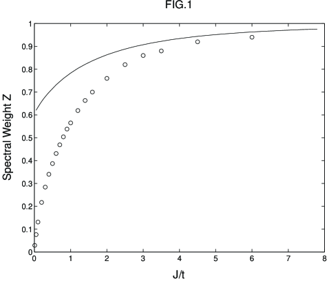
FIG. 1.: The spectral weight $Z$ for one hole located at the quasiparticle band minimun with momentum ${\bf k}_{0}=(\pm\frac{\pi}{2},\pm\frac{\pi}{2})$ as a function of $J/t$. The results of the intermediate-coupling theory are shown as the solid line, and open circles represent those obtained by SCBA  [9].

In the following, we will clarify the reason why the intermediate-coupling theory for the spin-polaron problem is not as successful as that for the lattice-polaron case. Notice that, after restricting to the subspace with one hole at momentum ${\bf k}$, as shown in Eqs.(45c) and (47) of Ref.[7], one arrives at the effective Hamiltonian for the boson operators [13]

$${\cal H}_{\bf k}\simeq\hbox{constant}+\sum_{\bf q}\epsilon_{\bf q}({\bf k})b_{\bf q}^{\dagger}b_{\bf q},$$ (25)

where $\epsilon_{\bf q}({\bf k})=\nu_{\bf q}+2\alpha\Omega({\bf k})$ can be considered as the renormalized energy spectrum of the spin waves in unit of $\omega$ in the rest frame of the hole at momentum ${\bf k}$. Hence, for ${\bf q}\to 0$, the renormalized energy spectrum $\epsilon_{\bf q}({\bf k})\to 2\alpha\Omega({\bf k})$, which is nonvanishing for a given ${\bf k}$; while the “ bare ” one, $\nu_{\bf q}\propto|{\bf q}|\to 0$. That is, a finite gap, $2\alpha\Omega({\bf k})$, is introduced into the excitation spectrum of the spin waves by this variational approach, even though the original excitation spectrum is gapless due to the Goldstone theorem [14] ! Thus the long-wavelength ( infrared ) properties of the system is altered qualitatively. This qualitative change in the excitation spectrum is not reasonable, because the correction to the spin wave energies by a single hole in a macroscopic AF background should be proportional to $1/N$, which would be negligible in the thermodynamic limit ! In the lattice-polaron case, although there is still a nonvanishing correction to the phonon energies [6], there is no qualitative change in the phonon energies by this approach, because only the longitudinal optical ( LO ) phonons are considered and the “ bare ” energy spectrum of these LO phonons can approxmately be taken as a positive constant. As claimed by Anderson [10], whether $Z$ is zero or not greatly depends on the infrared behavior of the system. Since the infrared behavior may not be faithfully described by this variational approach, it is reasonable that the intermediate-coupling theory may not predict the accurate value of $Z$ in the spin-polaron case.

For a further support of the above arguements, we present the results of the “induced spin gap”, $2\alpha\Omega({\bf k}_{0})$, as a function of $J/t$ in Fig.2. We find that, as $J/t$ decreases, the “induced spin gap” increases and invalidates the variational approach.

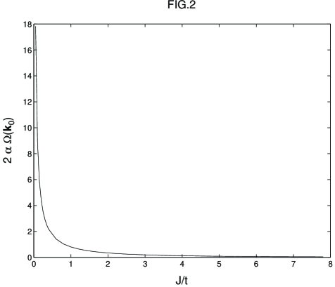
FIG. 2.: The “ induced spin gap ”, $2\alpha\Omega({\bf k}_{0})$, as a function of $J/t$.

In conclusion, within the intermediate-coupling theory, we show that the quasiparticle weight $Z$ is finite, and our results agree with those obtained by the self-consistent Born approximation [9] when $J/t\stackrel{{\scriptstyle>}}{{\sim}}1.6$. Because of the failure to describe correctly the infrared behavior of the system, this approach is not suitable for the study of the spectral weight of the spin-polaron case, especially when $J/t$ is small.

Acknowledgment: The author thanks Prof. T. K. Lee and Dr. M. C. Chang for their critical reading of the manuscript.

$\dagger$ E-mail address: mfyang@phys.nthu.edu.tw

REFERENCES

- [1] For reviews, see E. Dagotto, Rev. Mod. Phys. 66, 763 (1994); L. Yu, Z. B. Su, and Y. M. Li, Chin. J. Phys. ( Taipei ) 31, 579 (1993).
- [2] S. Schmitt-Rink, C. M. Varma and A. E. Ruckenstein, Phys. Rev. Lett. 60, 2793 (1988).
- [3] C. L. Kane, P. A. Lee and N. Read, Phys. Rev. B39, 6880 (1989).
- [4] For the review, see H. Fröhlich, in Polarons and Excitons, edited by C. G. Kuper and G.D. Whitfield ( Oliver and Boyd, Edinburg, 1962 ).
- [5] In fact, as mentioned in the article by L. Yu, Z. B. Su, and Y. M. Li [1], the analogy between the spin-polaron Hamiltonian, Eq.(2), and the Fröhlich Hamiltonian is not complete. For example, there is no “ bare ” hopping term of the holes in the spin-polaron case.
- [6] For the review, see D. Pine, in Polarons and Excitons, edited by C. G. Kuper and G. D. Whitfield ( Oliver and Boyd, Edinburg, 1962 ).
- [7] H. Barentzen, Phys. Rev. B 53, 5598 (1996).
- [8] E. Dagotto, A. Nazarenko, and M. Boninsegni, Phys. Rev. Lett. 73, 728 (1994).
- [9] G. Martínez and P. Horsch, Phys. Rev. B 44, 317 (1991).
- [10] P. W. Anderson, Phys. Rev. Lett. 64, 1839 (1990).
- [11] S. Sorella, Phys. Rev. B 46, 11670 (1992); E. Müller-Hartmann and C.I. Ventura, Phys. Rev. B 50, 9235 (1990); Q.F. Zhong and S. Sorella, Phys. Rev. B 51, 16135 (1995); Z. Y. Weng, Y. C. Chen, and D. N. Sheng, Preprint Cond-mat/9505124 (1995); Y. M. Li, N. d’Ambrumenil, L. Yu, and Z. B. Su, Phys. Rev. B 53, R14717 (1996).
- [12] In order to link to the treatment in Ref. [7], we will follow his notations as closely as possible.
- [13] The off-diagonal terms and the terms of higher than quadratic order in the boson operators are omitted, which are irrelevant to our present discussions.
- [14] J. Goldstone, Nuovo Cimento 19, 154 (1961). For a review, see P.W.Anderson, Basic Notions of Condensed Matter Physics ( Benjamin-Cummings, Menlo Park, Calif., 1984 ).