Deformation of polymer films by bending forces

Abstract

We study the deformation of nano–scale polymer films which are subject to external bending forces by means of computer simulation. The polymer is represented by a generalized bead–spring–model, intended to reproduce characteristic features of n–alkanes. The film is loaded by the action of a prismatic blade which is pressed into the polymer bulk from above and a pair of columns which support the film from below. The interaction between blade and support columns and the polymer is modelled by the repulsive part of a Lennard-Jones potential. For different system sizes as well as for different chainlengths, this nano–scale experiment is simulated by molecular dynamics methods. Our results allow us to give a first characterization of deformed states for such films. We resolve the kinetic and the dynamic stage of the deformation process in time and access the length scale between discrete particle and continuum mechanics behaviour. For the chainlengths considered here, we find that the deformation process is dominated by shear. We observe strangling effects for the film and deformation fluctuations in the steady state.

The film bending experiment

Nano–scale deformation processes are difficult to deal with. Typical systems may consist of $10^{4}$ to $10^{6}$ interacting particles but are still too coarse to apply continuum mechanics concepts directly. Computer simulation can fill the gap. In the following, we consider the effect of bending forces on polyethylene films with an equilibrium thickness of approximately 75 Å. Our perspective is somewhat different from that of a large group of computer studies on polymers which mainly address the bulk properties of the material. We do not restrict ourselves to equilibrium situations or perturbations around equilibrium, and it is not clear from the beginning if our results can be interpreted in terms of a linear viscoelastic response. As can be seen in Fig. 1, our simulations take place in a more complicated geometry than usual and the material undergoes considerable deformations. We consider surface effects and the interaction between polymer and rigid bodies which are pressed into the bulk. The problem as a whole also involves the search for a set of parameters which qualify for a concise description of what we are looking at.

The present line of work started with the indentation simulations of Hapke [1]. In these computer experiments, a rigid tip is pressed into the material to probe the resistance of the polymer surface. The indentation depth of the tip and a number of related parameters are recorded and analyzed. It became clear that this approach to nano–mechanics can be extended to more complicated situations. In addition to the investigation of nano–indentation and its connection to surface hardness and degradation, we can also contribute to fields of interest in nano–technology, like nano–bending, nano–forging, and nano–milling. In the next sections, we first describe the modelling of the bulk polymer and the interaction between polymer and solid bodies. We sketch the geometry of the computer experiment and mention some essential features of the simulation program. We then indicate a simple way to analyze the data from the computational deformation experiments and apply the method to data from various simulation runs. In particular, we look at the cross section displacement, the variable film thickness, the time development of the indentation depth, and the local density field in the bulk next to the invading body. Finally we summarize our findings and outline some possibilities for further research.

The polyethylene model

FIG. 1.: The building blocks of the computer experiment.

In computer experiments on the nano–mechanics of amorphous media, one typically has to model a number of different subsystems, including bulk polymer (chain molecules or polymer networks), free polymer surfaces, the interaction between polymer and tools (possibly manufactured from metal), and the behaviour of the tools themselves [1]. Each subsystem can be modelled on a different level of sophistication. We have to follow the motion of the monomers in the polymer chains, but are not interested in the dynamics of the electron gas in the metal tool. In what follows, we employ a standard model for chain molecules. New technical aspects of our work mainly concern the implementation of rigid geometries representing the solid tools and supports which can act onto the material. For the polymer, however, we use a common bead–spring model with some extensions to capture the essential features of polyethylene chains [1]. In addition to harmonic chain forces which keep the bond lengths next to the equilibrium value, we model the fluctuation of bond angles, again by a quadratic potential. Between monomers which do not participate in mutual bond length or bond angle interactions, Lennard–Jones forces are acting, both to model an excluded volume effect and to hold the polymer film together (the total energy in all our simulations is negative, the system is in a bound state). Note that we neglect any torsional potential in the present study. To be explicit, the Hamiltonian of the polyethylene model is of the form

$$H = H_{\rm\scriptstyle bondlength}+H_{\rm\scriptstyle bondangle}+H_{\rm\scriptstyle LJ}\,,$$ (1)

$$H_{\rm\scriptstyle bondlength} = \sum_{\rm\scriptstyle bonds}\frac{k_{b}}{2}\left(l_{\rm\scriptstyle bond}-l_{0}\right)^{2}\,,$$ (2)

$$H_{\rm\scriptstyle bondangle} = \sum_{\rm\scriptstyle angles}\frac{k_{\theta}}{2}\left(\cos\theta_{\rm\scriptstyle angle}-\cos\theta_{0}\right)^{2}\,,$$ (3)

$$H_{\rm\scriptstyle LJ} = \sum_{\rm\scriptstyle pairs\;of\atop\rm\scriptstyle monomers}4\epsilon\left[\left(\frac{\sigma}{r_{\rm\scriptstyle pair}}\right)^{12}-\left(\frac{\sigma}{r_{\rm\scriptstyle pair}}\right)^{6}\right]\,.$$ (4)

Models of this kind have been described at various places in the literature (e.g. Ref. [2], and, for specific details, Ref. [1]), so we can be short here. Let us only mention that we implement the Lennard–Jones interaction using the linked cell algorithm [2]. At the cutoff distance, we restore continuity in energy and force by appropriate shifts. The time stepping is done through the velocity form of the Verlet algorithm. The simulation program can be run in various major modes: pure molecular dynamics, molecular dynamics with velocity scaling (as a brute force approach to guarantee a constant temperature), Hybrid Monte Carlo (a combination of Monte Carlo and molecular dynamics, where the molecular dynamics part acts as the event generator), and Brownian dynamics (additive Langevin forces simulate the coupling to a heat bath). Also a Hoover thermostat has been implemented. The simulations reported on below were performed using pure molecular dynamics with the Hoover thermostat active. A number of parameters relevant to all these runs is given in Tab. I.

TABLE I.: Parameters of the polyethylene model.

Lennard–Jones energy, $\epsilon$	$8.3027\cdot 10^{-22}$ J	5.18 meV
Lennard–Jones length, $\sigma$	380 pm	3.8 Å
monomer mass (${\rm CH}_{2}$ group), $m$	$2.3248\cdot 10^{-26}$ kg	14 atomic units
unit of temperature, $\epsilon/k_{\rm B}$	60.1357 K
unit of mass density, $m/\sigma^{3}$	423.6687 ${\rm kg}/{\rm m}^{3}$	0.4237 ${\rm g}/{\rm cm}^{3}$
unit of time, $\left(m\sigma^{2}/\epsilon\right)^{1/2}$	2.0108 ps
unit of velocity, $\left(\epsilon/m\right)^{1/2}$	188.9822 m/s
unit of force, $\epsilon/\sigma$	2.1849 pN	1.36 ${\rm meV}/{\rm{\AA}}$
unit of spring constant, $\epsilon/\sigma^{2}$	$5.7498\cdot 10^{-3}$ N/m	0.36 ${\rm meV}/{\rm{\AA}}^{2}$
unit of pressure, $\epsilon/\sigma^{3}$	151.3103 bar	0.09 ${\rm meV}/{\rm{\AA}}^{3}$
temperature, $T$	361 K
bond length, $l_{0}$	152 pm	1.52 Å
spring constant (bond length), $k_{b}$	$5.7498\cdot 10^{1}$ N/m	3.59 ${\rm eV}/{\rm{\AA}}^{2}$
bending constant (bond angle), $k_{\theta}$	$8.3027\cdot 10^{-19}$ J	5.18 eV
simulation time step, $\Delta t$	2.0108 fs
external force on tool, $F$	0.25 nN	0.16 ${\rm eV}/{\rm{\AA}}$
box depth (y)	6.1 nm	61 Å
box heigth (z) (accessible, not filled)	15.2 nm	152 Å
equilibrium film thickness	$\approx\text{7.5 nm}$	$\approx\text{75 {\AA}}$

Interaction between polymer bulk and solid bodies

We model the interaction between polymer and solid bodies (tools and supports) solely by the repulsive ($r^{-12}$) part of the Lennard–Jones potential. Moreover, we use the same parameters (energy scale $\epsilon$ and length scale $\sigma$) as in the polymer bulk. At first glance, such an approach might not look appropriate at all and it certainly needs some justification. Our main argument is that we are just interested in what is independent of specific interaction models. Of course this presupposes that there are aspects of nano–deformation which do not depend on details like the exact potentials between organic molecules and metal surfaces. Work in the latter direction has been carried out by others [3], and it is certainly the next step to utilize their results. However, we are here concerned with issues which we think are both fundamental to the problem of nano–deformation and merely geometrical in nature. We want to observe what happens on a nano–scale if a material like polymer is displaced through the invasion of a compact body with a given shape. Within this approach, we cannot expect to resolve any interaction zones between polymer and tool. But what we miss are effects in a boundary layer on an even smaller scale which are not suspicious to dominate the overall behaviour. One should note, however, that we are not able to model any adhesion effects which become important if we pull the tool out of the polymer. A straightforward way to capture those aspects is to include the attractive part of the Lennard–Jones potential into the modelling.

In our computer experiments, we meet two types of rigid geometries which interact with the polymer film: fixed and movable ones. Fixed are the bottom and top plates and the two columns which support the film (see Fig. 1). They repell monomers but do not feel the reaction forces. The tool, a prismatic blade, belongs to the second category and is movable. It is modelled as a massive body of $10^{4}$ monomer masses which obeys Newtonian dynamics. The motion of the tool can therefore be naturally included into the overall time stepping algorithm for second order dynamics (here the velocity form of the Verlet algorithm). As a program option, the motion of the tool can also be controlled by distance [1]. This allows us to drive the tool to a certain position in the bulk and to probe the reaction forces, but we did not use this feature here. A number of tool parameters can be varied, including the tip radius (here we use an acute tip with a formal tip radius of zero), the tip opening angle (here 30 degrees), the insertion force (here 0.25 nN), the tip mass (here $1.4\cdot 10^{5}$ atomic units = $2.3248\cdot 10^{-22}$ kg), and the tool’s angle of attack (here straight from above). In any case, whether by prescribed motion or under the action of an external force, pressing the tool into the bulk adds energy to the polymer subsystem. The use of some kind of thermostat is therefore mandatory to achieve an isothermal simulation for the polymer. In Fig. 1, a cross section through the experiment in the x/z–plane is shown. As mentioned, the boundary in the height (z) direction consists of repelling plates. In the lateral directions, refered to as width (x) and depth (y), we use common periodic boundary conditions. The depth is a neutral direction according to this setup and is exploited for additional averaging.

Results from the computer experiments

FIG. 2.: A small system of width 60 Å with 8220 chains of length 60, shown 1.6 ns after the start of the bending experiment.

FIG. 3.: A medium system of width 120 Å with 16400 chains of length 20, shown 0.8 ns after the start of the bending experiment.

We report on computational bending experiments for systems of three different sizes and refer to them as to the small (Fig. 2), medium (Fig. 3), and large configurations. Simulation parameters which apply to all systems have been summarized in Tab. I. The systems differ in their width and the number of monomers considered. For each size, results for chains built from 20 and 40 monomers (small system also 60 monomers) are available. Note that for each configuration size, we keep the number of monomers constant, so going to longer chains means a reduction in the chain number. More details are given in Tab. II.

TABLE II.: The various simulated polyethylene systems.

Small polyethylene system.
number of chains (chainlengths 20, 40, and 60)	410, 205, and 137
number of monomers	8200
box width (x)	61 Å
total simulation time	$\approx\text{4 ns}$
Medium polyethylene system.
number of chains (chainlengths 20 and 40)	820 and 410
number of monomers	16400
box width (x)	122 Å
total simulation time	$\approx\text{1 ns}$
Large polyethylene system.
number of chains (chainlengths 20 and 40)	1640 and 820
number of monomers	32800
box width (x)	243 Å
total simulation time	$\approx\text{? ns}$

The characterization of deformation

Although the blade is driven by a force of only 0.25 nN, the polymer film undergoes considerable deformations, especially in the medium and large systems. In continuum mechanics, the standard method to describe any deformation is to use three–dimensional vector fields. In order to proceed that way, one has to define so–called material points which can be labeled and followed in space during the deformation history. One might think about them as marked pieces of matter. The vector field then encodes the difference in position of the material points between some reference and the current configuration. In our situation, we must be careful and cannot naively use a monomer or the center of gravity of a polymer chain as a material point. In the deformed steady state, chain diffusion processes carry on, and material points would continue to move. Note, however, that in theoretical treatments of viscoelasticity [4, 5], one follows the motion of monomers indeed, since when the pressure tensor is set up, one must also consider the forces which are mediated by the polymer bonds. A practicable alternative to characterize the deformed state is to calculate collective quantities based on the monomer positions. We proceed this way and divide the system into slices in the width direction. In each slice, we compute the center of the cross section,

$$c(x)=\frac{1}{N(x)}\sum_{\rm\scriptstyle monomers\atop\rm\scriptstyle in\;slice}z_{\text{monomer}}\,,$$ (5)

as the average of the monomer $z$ coordinates in the slice at position $x$ ($N(x)$ is the total number of monomers in that slice). The set of these centers plotted over the width coordinate constitute what we call the bending line. Furthermore, we consider the radius of gyration of the cross section,

$$r^{2}(x)=\frac{1}{N(x)}\sum_{\rm\scriptstyle monomers\atop\rm\scriptstyle in\;slice}\left(z_{\text{monomer}}-c(x)\right)^{2}\,.$$ (6)

For films with approximately constant monomer density over the height direction (and we take that for granted), this is a measure for the local film thickness and a plot of $r(x)$ allows to detect regions of film widening and strangling. Note that both definitions only use the $z$ coordinates of the monomers, since $x$ represents the independent coordinate, and the $y$ direction is neutral and used for averaging. Note, however, that based on quantities which are solely averages over single monomer coordinates (we may call this statistics on points) we cannot decide whether elastic bending or elastic or viscous shear effects dominate the deformation of the polymer film. In order to proceed, the relative positions of material points (which define lines or planes in some reference configuration) must be considered. To discern elastic from viscous effects, we must resolve the mapping of lines and planes by the deformation process in time.

Bending lines

A snapshot of one small configuration under bending is displayed in Fig. 2. In order to show some layers of monomers in the total front view, each monomer ball has been drawn with a radius smaller than its Lennard–Jones radius of 3.8 Å. The section under the magnifying glass, however, uses this radius for the monomers.

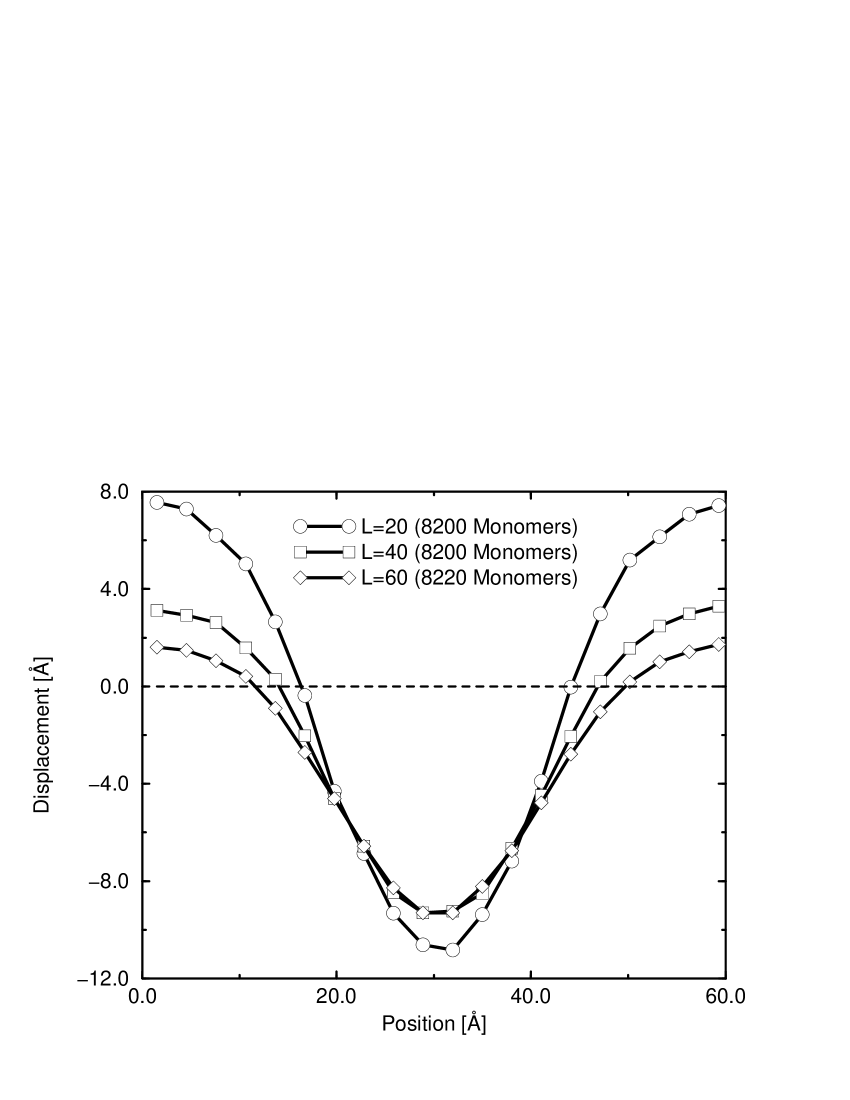
FIG. 4.: Bending lines for small systems.

The bending lines for small systems of various chainlengths are plotted in Fig. 4. Note the different scales on both axes. For systems of width 60 Å, we find a maximum displacement of about 10 Å, corresponding to a ratio of 6:1. We see that the system with the shortest chains undergoes the largest deformation and that the material is not only bent below the zero line but also displaced to both sides of the invading tool. The difference between chainlength 20 and 40 is more prominent than between 40 and 60. This should be compared to the behaviour of medium systems, one of which is shown in Fig. 3.

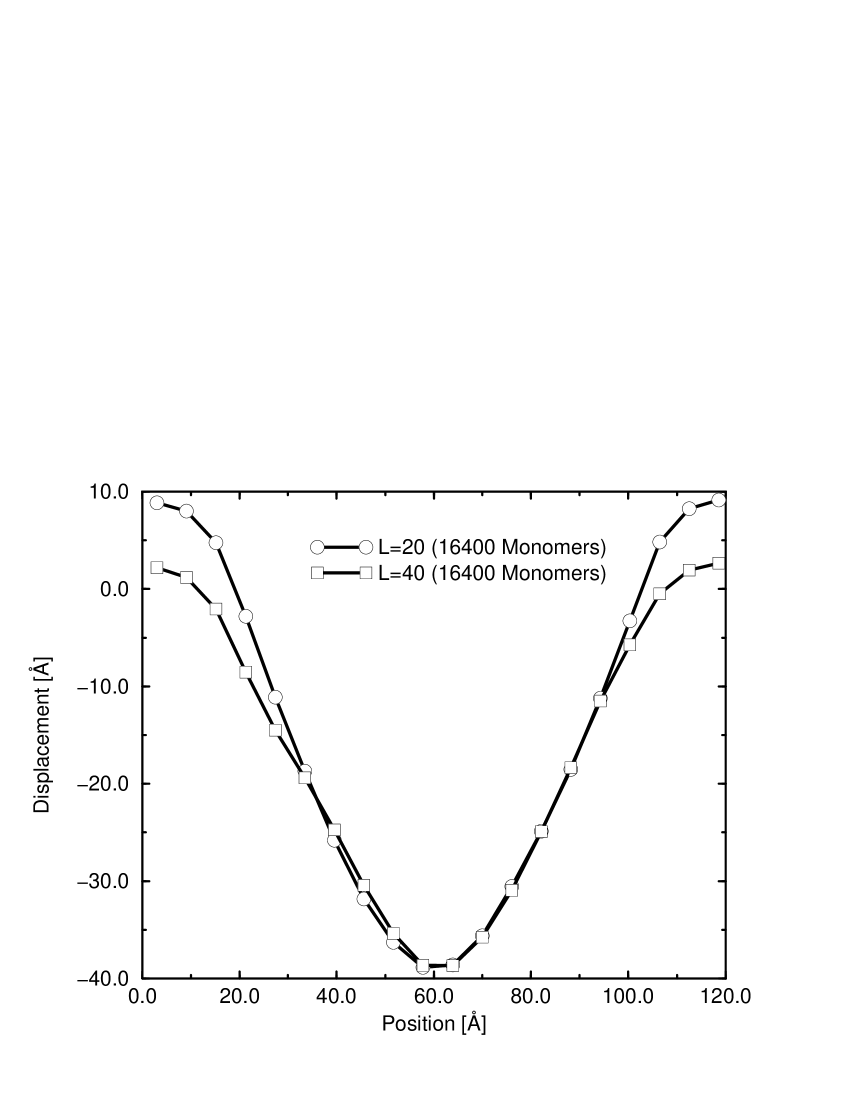
FIG. 5.: Bending lines for medium systems.

Their bending lines, Fig. 5, are more curved, the ratio between width and maximum displacement is changed to 3:1. The difference between the bending lines for chainlength 20 and 40 is reduced with respect to the small configurations. Already from these obervations we can infer that with the small configurations we merely perform indentation experiments [6], at least for an applied force of 0.25 nN. Due to the aspect ratio of the small systems, there is little space for material displacement between the two support columns. On the other hand, for the medium systems, a look at Fig. 3 suggests that the deformation is mainly limited by the constraint imposed by the lower plate (which repells the polymer). We have already exceeded the terminal relaxation time [7], and the polymer is sheared like a liquid. For further simulations, we are urged to resolve the initial, kinetic phase of the bending experiment more carefully if we want to observe any elastic effects in accordance with the classical notion of bending.

Film strangling

FIG. 6.: Radii of gyration for small systems.

The thickness of the polymer film locally changes under the action of the invading tool. This can be concluded from plots of the radius of gyration over the width direction. Fig. 6 summarizes the situation for the small systems. The equilibrium value for the radius in this plot is around 20 Å. We find film thickening at the sides and thinning in the center, below the tool. This fits into our picture that these simulations correspond to indentation experiments were material does not only move into the cavity between the support columns but also gets displaced to both sides of the tool. Again there is a significant difference between chains of length 20 and of length 40. The longest chains show the smallest displacement effects.

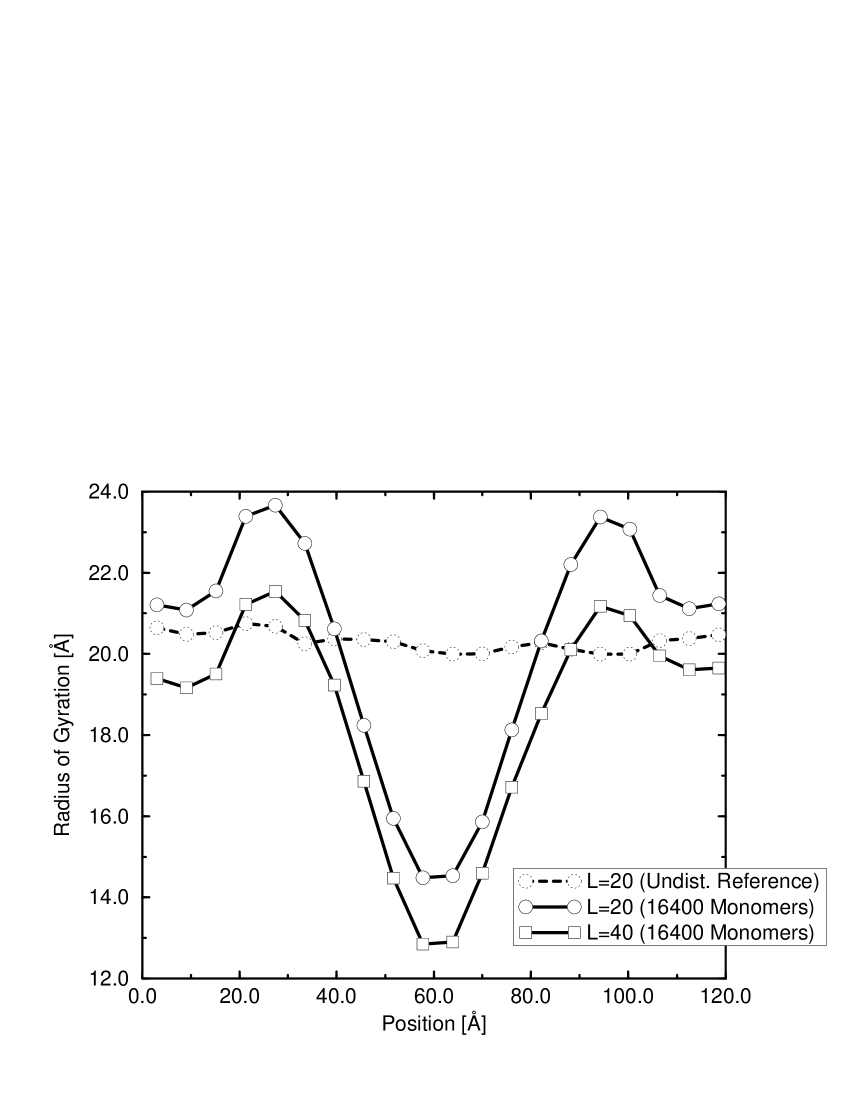
FIG. 7.: Radii of gyration for medium systems.

For medium systems we plot the strangling effects in Fig. 7. They are more pronounced than for small ones. Also observe the clearly visible thickening regions to both sides of the tool. Above the support columns, the film becomes thinner again. This effect is plausible, since for systems with larger width, the exact geometrical shape of the interacting body (tool or support) ceases to matter and the interaction is reduced to an overall displacement effect.

Indentation depth

The indentation depth measures the movement of the tool’s tip from its starting position just above the polymer surface into the bulk. The sign convention follows the orientation of the height axis and the indentation counts negative if the tool moves down. In Fig. 8, we show the time development of this quantity for three small systems with chainlength 20, 40, and 60. We conjecture that the shorter the chains are, the lower lies the first minimum of the curve (reflecting the higher flexibility of shorter chains) but the higher is the average tip position in the steady state (finally indicating a higher resistance against indentation of the shorter chains). This is what also has been found in our dedicated indentation simulations [6]. Moreover, the position fluctuations may well increase with decreasing chainlength. To clarify the connection between the tip position and the deformation of the polymer film, we have to think about some appropriate norm of the displacement field. One such quantity certainly is the maximum displacement found for some cross section (the minimum of the bending curves). For medium configurations, this quantity together with the tip position is plotted in Fig. 9 for increasing time. We see that this norm of the deformation state instantly follows the external forcing, meaning that no delay effects which indicate viscoelasticity can be observed on the time scale under consideration. Moreover, this figure demonstrates that compared to small systems, the relative steady state deformation fluctuations become reduced and that the difference between chainlength 20 and 40 disappears in the steady state.

FIG. 8.: Time dependence of the tool indentation depth for small systems.

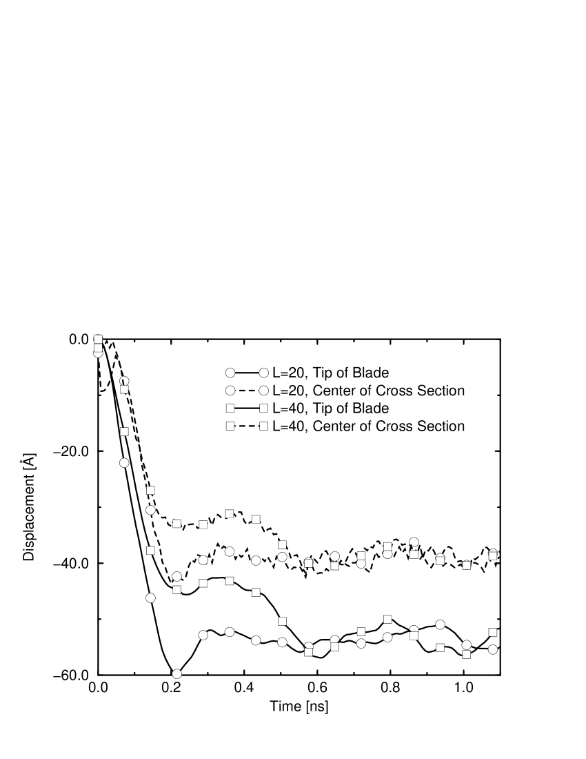
FIG. 9.: Connection between indentation depth and section displacement.

From Fig. 8 we can estimate that the tool moves about 20 Å in 1 ns. This corresponds to an impact velocity of 2 m/s. Similarly, from Fig. 9 the estimate is 60 Å in 0.2 ns, which means a tool impact with 30 m/s or roughly 100 km/h. These time scales should be compared to certain relaxation times which characterize equilibrium diffusion as defined in Ref. [8]. At the time $\tau_{3}$ in particular , determined by long term equilibrium runs and tabulated in Tab. III, the mean square displacement of mid chain monomers in the chains’ center of mass system is on average the same as the mean square displacement of the center of mass itself (the former asymptotically approaches the square of the radius of gyration whereas the latter increases linearly in time). We see that especially for longer chainlengths there is no strict separation of time scales (diffusion and indentation dynamics), but the polymer has some time to adapt to the constraints imposed by the tool. One is tempted to propose a szenario with three time stages: the first stage includes the impact process, during the second stage, the tool performs damped oscillations around some average steady state position (which may, however, drift on some longer time scale), and in the third stage, the polymer bulk restores equilibrium. Note that in this paper we loosely refer to the “steady state” as to the time when impact phenomena have faded out.

TABLE III.: Simulation values for the equilibrium relaxation time $\tau_{3}$.

chainlength	time scale $\tau_{3}$ (see Ref. [8])
20 monomers	8 ps
40 monomers	50 ps
60 monomers	240 ps

Density profiles

If a solid body invades some yielding material, besides the gross deformation also local effects are worth to investigate, especially if one expects some transient phenomena or local defects leading to failure (film fracture or strangling). As a first step towards an accurate spatial resolution of the interaction zone between tool and polymer, the polymer mass density found in shells of increasing distance from the tool’s tip is plotted in Fig. 10. This plot combines small and medium systems. For all systems, the density increases monotonically from zero (next to the tool) to its bulk value.

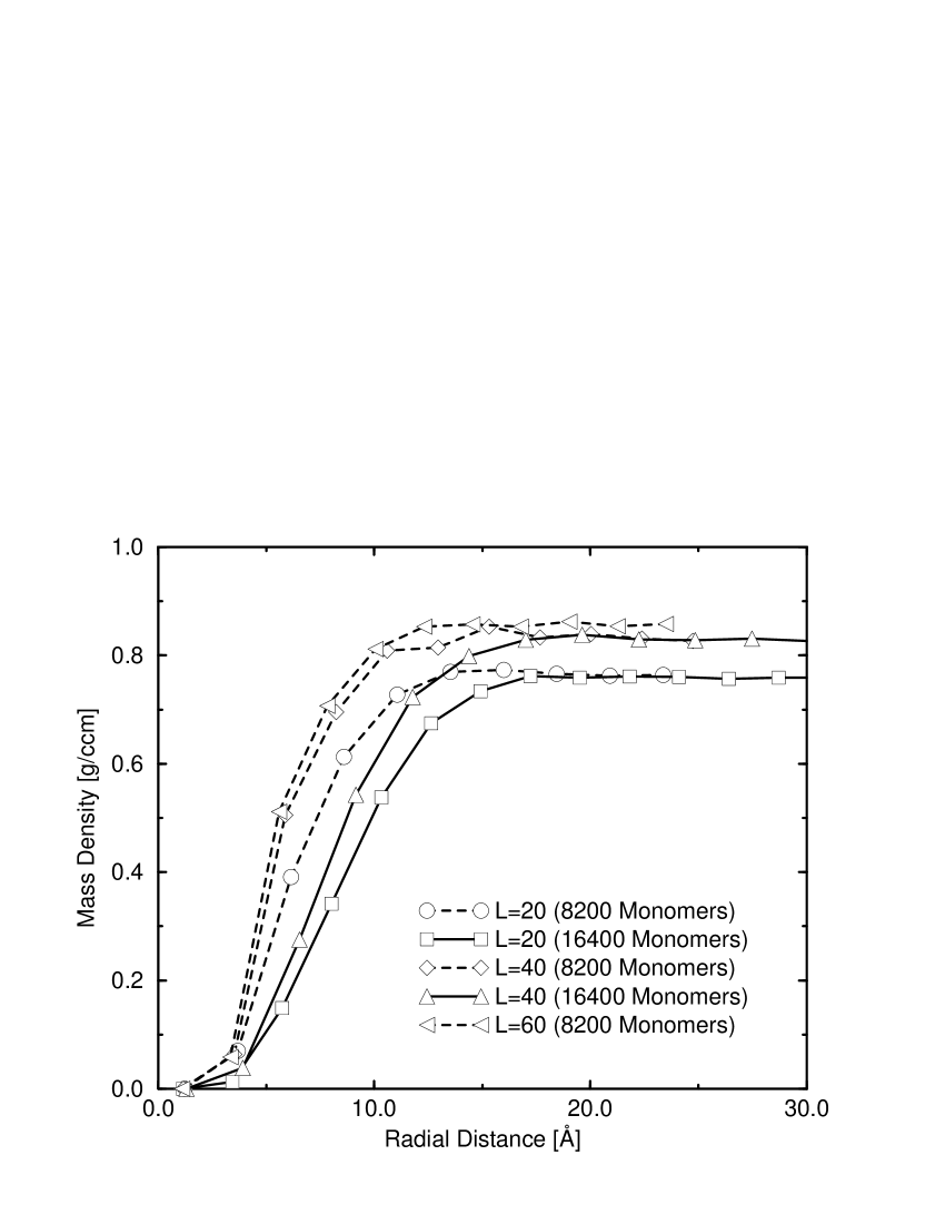
FIG. 10.: Radial mass density distribution.

For the same chain length, both the small and the medium configurations reach the same plateau value of the density which gives us additional confidence that the systems are large enough to observe bulk behaviour. Note that for small systems the diameter of the shells is limited since otherwise parts of the shell lie outside the region filled with material. For a given system size, we find that the longer the chains, the higher the bulk density and the steeper the flank of the density profile. For the medium systems, the profiles are somewhat flatter, since in larger systems the material bends down and has more room to move aside. Recall that the tool exerts a purely repelling force with a length scale of $\sigma=\text{3.8 {\AA}}$ (which is the same as the Lennard–Jones radius of the monomers). The plateau density has been restored at a distance of roughly $4\sigma\approx\text{15 {\AA}}$ which should be compared to the approximate film thickness of $20\sigma\approx\text{75 {\AA}}$.

Conclusion and outlook

We have demonstrated that the nano–mechanics of amorphous media like polymer films can successfully be dealt with by computer simulation. The length scale considered here is of particular interest, since we treat a number of chains large enough to constitute some bulk, but, on the other hand, too small to justify the naive application of continuum mechanics. We have reported on illustrative but nevertheless fundamental aspects of nano–deformation: displacement of cross sections, film strangling, and indentation depth. These are the first steps towards the kinematical characterization of the deformation process. We also took a preliminary look at the local reaction of the material to the indentation and displayed the mass density in the polymer bulk at increasing distance from the tool.

A step to be undertaken next is to resolve the non–equilibrium forces which emerge during the deformation process, both in space and time. It must clarified whether the notion of a local deformation field and the concept of a stress can be suitably modified and adapted to the present situation. We also must be explicit about the various dynamical processes taking place in the computer experiment (diffusion, steady state deformation fluctuations) and especially about their relaxation times under non–equilibrium conditions. Of particular interest is the relation between tool velocity and chain movement. A simplified picture of the deformation process consisting of certain time stages (three of them have been suggested above) can then be set up. Finally, the long time behaviour of the polymer system under load is of interest. One possible criterion to monitor are the non–equilibrium forces in the polymer bulk caused by the invading tool. For long times, these forces relax. It is highly probable however, that slow creep processes, controlled by viscous steady state forces, carry on. After the descriptive work is accomplished, one will be tempted to average over the granularity of single chains and to set up a smoother model for nano–deformation. An interesting prospect for theoretical work is then to derive what corresponds to the constitutive equations of continuum mechanics for such a model.

REFERENCES

- [1] Th. Hapke, Simulation mikromechanischer Eigenschaften von amorphen makromolekularen Gläsern am Beispiel von Polyethylen, Diplomarbeit am Institut für Theoretische Physik der Universität Heidelberg, 1995.
- [2] M. P. Allen and D. J. Tildesley, Computer Simulation of Liquids (Clarendon Press, Oxford, 1987).
- [3] A. K .Chakraborty, H. T. Davis, and M. Tirrell, J. Polym. Sci. A: Polym. Chem. 28, 3185 (1990); J. S. Shaffer, A. K .Chakraborty, M. Tirrell, H. T. Davis, and J. L. Martins, J. Chem. Phys. 95, 8616 (1991); T. K. Xia, J. Ouyang, M. W. Ribarsky, and U. Landman, Phys. Rev. Lett. 69, 1967 (1992); W. D. Luedtke and U. Landman, Comp. Mat. Sci. 1, 1 (1992).
- [4] M. Doi and S. F. Edwards, The Theory of Polymer Dynamics (Clarendon Press, Oxford, 1986).
- [5] R. B. Bird, R. C. Armstrong, O. Hassager, and C. F. Curtiss, Dynamics of Polymeric Liquids, vol. 1 (Fluid Mechanics) and vol. 2 (Kinetic Theory) (Wiley, New York, 1977).
- [6] Th. Hapke, A. Linke, and D. W. Heermann (to be published).
- [7] P.–G. de Gennes, Scaling Concepts in Polymer Physics (Cornell University Press, Ithaca, 1979).
- [8] W. Paul, K. Binder, D. W. Heermann, and K. Kremer, J. Chem. Phys. 95, 7726 (1991).