Modelling of amorphous polymer surfaces in computer simulation

Abstract

We study surface effects in amorphous polymer systems by means of computer simulation. In the framework of molecular dynamics, we present two different methods to prepare such surfaces. Free surfaces are stabilized solely by van–der–Waals interactions whereas confined surfaces emerge in the presence of repelling plates. The two models are compared in various computer simulations. For free surfaces, we analyze the migration of end–monomers to the surface. The buildup of density and pressure profiles from zero to their bulk values depends on the surface preparation method. In the case of confined surfaces, we find density and pressure oszillations next to the repelling plates. We investigate the influence of surfaces on the coordination number, on the orientation of single bonds, and on polymer end–to–end vectors. Furthermore, different statistical methods to determine location and width of the surface region for systems of various chain lengths are discussed and applied. We introduce a “height function” and show that this method allows to determine average surface profiles only by scanning the outermost layer of monomers.
Keywords: Polymer surfaces; Computer simulation; Surface modelling and characterization.

Introduction

The technological applicability of polymeric materials depends in a number of important cases on the polymer’s surface properties: the surface roughness determines the friction coefficient, cracks emerging from the surface influence the material’s durability, and surface defects reduce the transparency of polymeric panes. At the same time, the experimental and manufacturing techniques advance to smaller and smaller scales. Nowadays one can pursue mechanical effects on the nano–scale. This opens new, challenging, and exciting roads for academic research and promising prospects for industrial applications. Nano–mechanics influences the design of computer chips and is fundamental for new developments like miniaturized optical devices and nano–engines. A related topic is the mechanics of very thin films [1] with thicknesses in the nano–range. But again, it is not just the bulk behaviour that decides about the nano–technological applicability of a certain material but its surface properties. The nano–scale processes that lead to macroscopically relevant surface–related phenomena like friction, wear, hardness, and certain types of material failure like surface degradation are scarcely understood from the theoretical point of view. In some cases, phenomenological theories exist [2] which attempt to systematize the various experimental observations. A fundamental understanding, however, tentatively based on fundamental nano–scale processes, is lacking. The reason is that on this scale, the number of mutually interacting particles is very high, but the system is still too coarse to apply continuum mechanics in a straightforward way. Some simplifications can be made in the case of crystalline solids but amorphous systems like polymer glasses still represent a major challenge. Techniques from computational physics can help to deal with the many degrees of freedom involved [3].

In ongoing work, we intend to address several basic questions that pertain to the understanding of nanoscopic amorphous systems in conjunction with tribological and surface effects like friction, wear, and hardness. Our investigation is mainly restricted to polymeric materials. Crystalline solids have been studied in a beautiful series of pioneering papers by Landman et al. [4]. In the present contribution, we concentrate on the preparation of polymer surfaces in the framework of computer simulation. We are furthermore concerned with the detailed characterization of important surface properties. This is a necessary foundation to correctly interpret our findings from a large number of dedicated polymer surface indentation simulations [5]. These simulations provide a prototype nano–scale experiment to probe surface hardness, friction, and damage mechanisms. Related to these activities are computer studies on the deformability of nano–scale polymeric films [6].

Polymer and surface modelling

For the polymer chains, we use a united atom model in conjunction with Newtonian dynamics. In addition to harmonic chain forces which keep the bond lengths next to the equilibrium value, we model the fluctuation of bond angles, again by a quadratic potential. Between monomers which do not participate in mutual bond length or bond angle interactions, Lennard–Jones forces are acting, both to model an excluded volume effect and to hold the polymer system together. Note that we neglect any torsional potential in the present study. To be explicit, the Hamiltonian of the model is of the general form

$$H = H_{\rm\scriptstyle bondlength}+H_{\rm\scriptstyle bondangle}+H_{\rm\scriptstyle LJ}\,,$$ (1)

$$H_{\rm\scriptstyle bondlength} = \sum_{\rm\scriptstyle bonds}\frac{k_{b}}{2}\left(l_{\rm\scriptstyle bond}-l_{0}\right)^{2}\,,$$ (2)

$$H_{\rm\scriptstyle bondangle} = \sum_{\rm\scriptstyle angles}\frac{k_{\theta}}{2}\left(\cos\theta_{\rm\scriptstyle angle}-\cos\theta_{0}\right)^{2}\,,$$ (3)

$$H_{\rm\scriptstyle LJ} = \sum_{\rm\scriptstyle pairs\;of\atop\rm\scriptstyle monomers}4\epsilon\left[\left(\frac{\sigma}{r_{\rm\scriptstyle pair}}\right)^{12}-\left(\frac{\sigma}{r_{\rm\scriptstyle pair}}\right)^{6}\right]\,.$$ (4)

The Lennard–Jones interaction is implemented with a cutoff of $2.5\,\sigma$ and appropriate potential and force shifts are used to retain continuity. We use molecular dynamics methods to compute the motion of the monomers. Models of this kind are described at various places in the literature [7]. We intend to capture some essential features of polyethylene chains and appropriate model parameters are compiled in Tab. I (see also Ref. [8]).

TABLE I.: Parameters of the polyethylene model.

Lennard–Jones energy, $\epsilon$	$8.3027\cdot 10^{-22}$ J	5.18 meV
Lennard–Jones length, $\sigma$	380 pm	3.8 Å
monomer mass (${\rm CH}_{2}$ group), $m$	$2.3248\cdot 10^{-26}$ kg	14 atomic units
unit of temperature, $\epsilon/k_{\rm B}$	60.1357 K
unit of mass density, $m/\sigma^{3}$	423.6687 ${\rm kg}/{\rm m}^{3}$	0.4237 ${\rm g}/{\rm cm}^{3}$
unit of time, $\left(m\sigma^{2}/\epsilon\right)^{1/2}$	2.0108 ps
unit of velocity, $\left(\epsilon/m\right)^{1/2}$	188.9822 m/s
unit of force, $\epsilon/\sigma$	2.1849 pN	1.36 ${\rm meV}/{\rm{\AA}}$
unit of spring constant, $\epsilon/\sigma^{2}$	$5.7498\cdot 10^{-3}$ N/m	0.36 ${\rm meV}/{\rm{\AA}}^{2}$
unit of pressure, $\epsilon/\sigma^{3}$	151.3103 bar	0.09 ${\rm meV}/{\rm{\AA}}^{3}$
temperature, $T$	301 K and 361 K
bond length, $l_{0}$	152 pm	1.52 Å
bond angle, $\theta_{0}$	109.47${}^{\text{\,o}}$	$\cos\theta_{0}=-1/3$
spring constant (bond length), $k_{b}$	$5.7498\cdot 10^{1}$ N/m	3.59 ${\rm eV}/{\rm{\AA}}^{2}$
bending constant (bond angle), $k_{\theta}$	$8.3027\cdot 10^{-19}$ J	5.18 eV
simulation time step, $\Delta t$	2.0108 fs

FIG. 1.: The confined polymer surface (at the top of the bulk). The horizontal line of the frame represents the repelling plate. The monomers are drawn with their Lennard–Jones radius $\sigma$. In the lateral directions, periodic boundary conditions apply.

FIG. 2.: The free polymer surface (at the top of the bulk). The horizontal line of the frame is out of the interaction range. The monomers are drawn with their Lennard–Jones radius $\sigma$. In the lateral directions, periodic boundary conditions apply.

We employ two alternative methods to prepare amorphous polymer surfaces. The confined polymer surface, Fig. 1, is realized by plates that repell the monomeric units and thereby restrict the polymer to a certain region in space. This gives rise to a surface model which is mainly characterized by its smoothness. In the simulations, we set up the united atom model with periodic boundary conditions in the $x$– and $y$–direction. In the $z$–direction, we put two repelling plates at a distance chosen such that the resulting bulk density of the polymer system settles to the desired value. The plates interact with the polymers through the repelling ($r^{-12}$) part of the Lennard–Jones potential. The other alternative, Fig. 2, is the free polymer surface. Here the polymer bulk is held together solely by the overall attracting intermolecular van–der–Waals interactions. Individual chains may evaporate or condensate. The emerging surfaces are rougher than in the confined case. We suggest that the confined model applies to the interface between the polymer and a comparatively rigid material like a metal. Such surfaces may also be formed on explosion pressed materials. On the other hand, the free surface is capable to model the interface between the polymer and a (dilute) medium where any mutual interactions can be neglected (in effect, it is the interface to a vacuum).

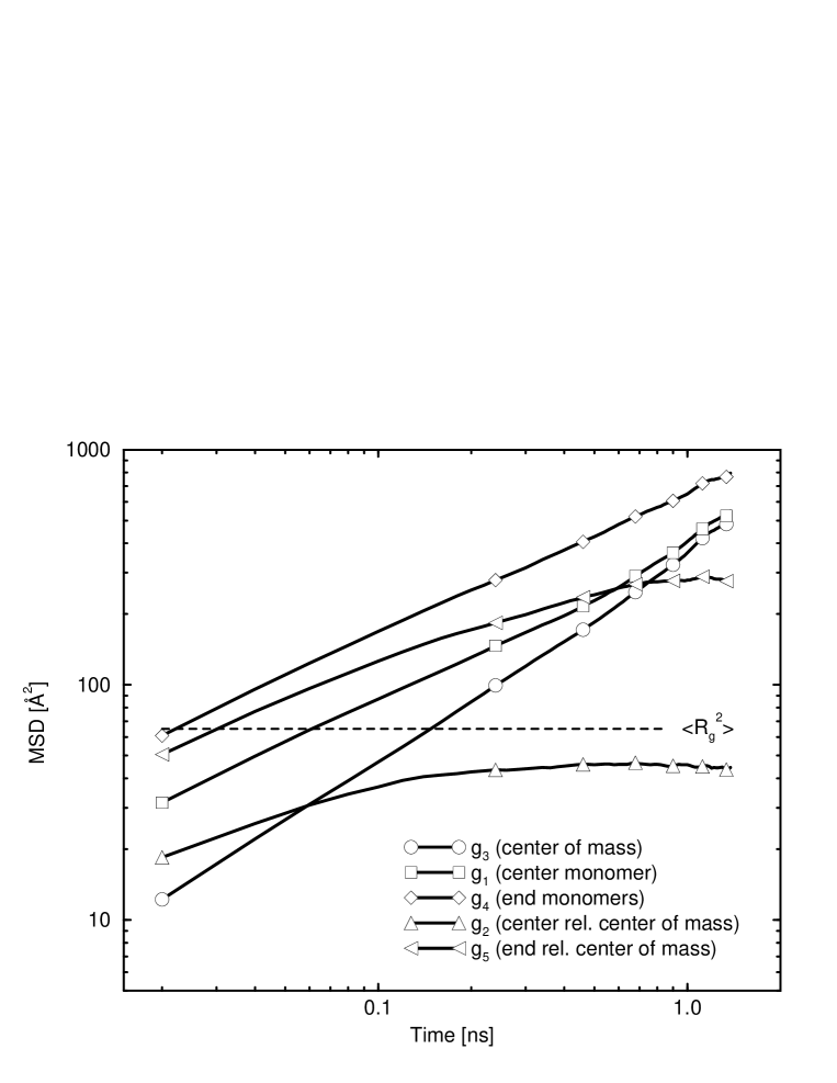
FIG. 3.: Various measures of the mean square displacement (MSD). In particular, $g_{1}$ is the MSD of the center monomers, $g_{2}$ is the same but relative to each chain’s center of mass, $g_{3}$ is the MSD of the chains’ center of mass, $g_{4}$ is the MSD of the end monomers, and $g_{5}$ is the same but again relative to each chain’s center of mass. The chain length is $N=40$ and only every tenth sample point is marked by a symbol.

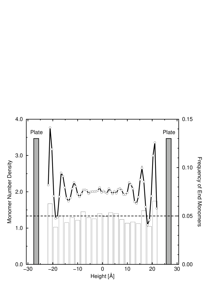
FIG. 4.: Distribution of density and end–monomers for the confined surface. Shown is the number density of monomers (solid curve, left axis) and the relative frequency of chain–end monomers (bar chart, right axis) in slices parallel to the surface. The polymer system is monodisperse and contains 205 chains of $N=40$ monomers each. The horizontal dashed line indicates the mean value for chain–ends: $\text{2 ends}/\text{40 monomers}=0.05$. Also shown is the location of the confining plates at both sides.

All simulations to probe surface properties are perfomed at reduced temperatures of $T^{*}=T/(\epsilon/k_{\rm B})=5.0$ (confined system) or $6.0$ (free system). These temperatures correspond to $301$ or $361$ Kelvin which is above the melting temperature of real polyethylene. We stress that our simulations are not yet supposed to fully mimic real polyethylene (it has been demonstrated, however, that much can be achieved by carefully tuning the parameters of united atom models [8]). The chain lengths are still too short and we treat chain–end monomers like mid–chain monomers. We also neglect the torsional potential (the rotation about C–C axes is not restricted). The high temperature helps to ensure that in feasible simulation times, the chains travel several radii of gyration in order to guarantee correct thermodynamic properties. To check this, various mean square displacement measures as defined in Ref. [9] are shown in Fig. 3. Indication that the chain in its entirety has moved through the matrix comes from the relative displacements of the inner monomers relative to the center of mass motion ($g_{2}$) and the outer monomers relative to the center of mass motion ($g_{5}$). The cross–over points define charateristic time–scales of the system. The presence of the cross–over points in Fig. 3 indicates that the simulation time scale is sufficiently long compared to the short–order relaxation times. Note that the data for all the figures to follow represent averages over a great number of system configurations which have been sampled from simulations which extend over a span of time comparable to that in Fig. 3. For each chain length ($N\!=\!20$, $40$, $60$, and $80$), the simulation follows 8200 monomers over 1.4 nanoseconds. If not otherwise indicated, the results given are for the chain length $N\!=\!40$.

Confined polymer surfaces

In the case of the polymer system with confined surfaces, the plates are rapidly brought from infinity to a distance such that the monomer number density in the resulting box is $\rho_{\text{bulk}}=2.0$. The shock results in a distribution of the density in the $z$–direction (system height) as shown in Fig. 4. These typical periodic changes of the density distribution close to the surface [10] are due to the external pressure produced by the plates, which leads to a local partial crystallization. The same behaviour has been found in simulations analyzing surface phenomena [11] and studied in the context of one long chain between two parallel plates [12]. The chains experience strong packing constraints as well as a loss in entropy that must show up also in the surface properties that can be observed during indentation.

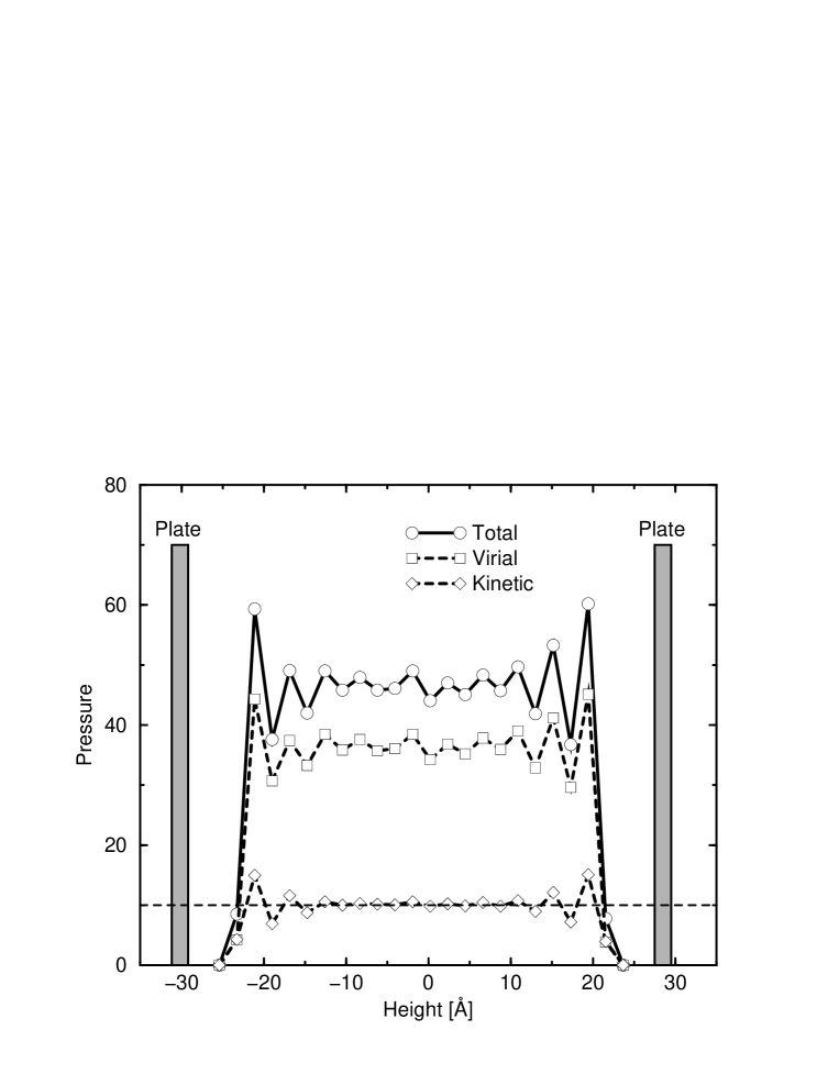
FIG. 5.: The pressure distribution vs. the height direction for the confined surface model (pressure in reduced units). The total pressure is the sum of the virial and the kinetic contribution. Also shown is the location of the confining plates at both sides. The dashed horizontal line indicates the expected value for the kinetic (ideal) part: $p^{*}_{\text{ideal}}=\rho^{*}T^{*}\approx 2.0\cdot 5.0=10.0$.

Fig. 4 also probes the chain–end enrichment effect for confined surfaces. Such an enrichment has been noticed by Wang and Binder [13] in a lattice model. Shown with the density profile is the relative frequency of end–monomers. This is computed by defining slices of height $d$ in the $z$-direction and dividing the number of chain ends by the total number of monomers within each slice. The resulting relative frequency is fairly independent of the slice height $d$. We conclude from the figure that there is no appreciable chain–end enrichment at confined surfaces. This is in accordance with the fact that there are no energetic or entropic reasons for the end–monomers to gather in the vicinity of the plates (see the discussion for free surfaces below). The constraints imposed by the plates can favour a high positive virial contribution to the pressure. Remember that for confined surfaces, the volume and therefore the mean density of the simulation system is prescribed. The high pressure in Fig. 5 can be traced back to repelling intermolecular interactions caused by dense packing.

Free polymer surfaces

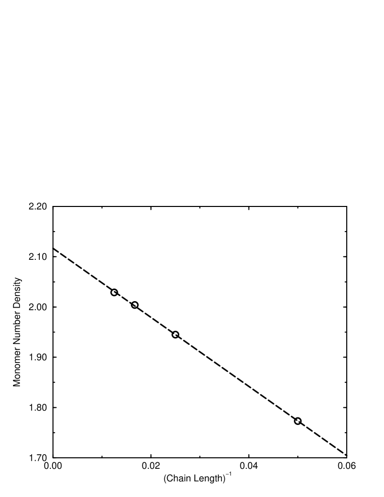
FIG. 6.: The monomer number density in the bulk (open circles) for different chain lengths (20, 40, 60, and 80 monomers) plotted vs. the reciprocal chain length in the free surface model. The dashed line is a linear fit to the data points. Its intercept with the $y$–axis yields $\rho^{*}_{\text{bulk}}(N\to\infty)\approx 2.12$ ($\text{slope}\approx-6.87$).

To study the effects of a rougher and presumably more realistic surface, we set up a free system with periodic boundary conditions in $x$– and $y$–direction and free boundary conditions in $z$–direction. The polymer bulk is held together by the attractive part of the inter–molecular Lennard–Jones interaction. At the beginning, this system can be prepared like a confined one with two repelling plates in the $z$–direction. This is mainly done to bring the polymer bulk initially into a regular shape. By previous experience, the density during the constrained phase is chosen close to the bulk density of a free system. After a time, the plates are removed and the system is free to relax into the surrounding vacuum. Another possibility is to start with a periodic box completely filled with polymer. This system is run over a relaxation phase which is finished when the chains have diffused over at least two radii of gyration. After that the periodic boundary condition in the $z$–direction is removed and the box is rendered three times as high as before. The polymer film is placed into the middle of the box and the simulation continues. The density profiles quickly approach their stationary shape and we made sure that their bulk or plateau values are independent from the initial density in the periodic box. Especially for longer chains this gives a good criterion that the dynamics have approached the equilibrium stage. The bulk densities found for varying chain lengths are summerized in Fig. 6. The reason for the different bulk densities is the ratio of chain–end to mid–chain monomers. In our model, the effective volume of chain–end monomers is higher than that of mid–chain monomers, since end–monomers with only one bond need more room than those with two bonds (the Lennard–Jones range $\sigma$ is the same for all monomers and longer than the bond length $l_{0}$) and also since the end–monomers have a higher mobility (entropic effect). For different chain lengths, the bulk densities are interpolated by the formula

$$\rho_{\text{bulk}}=\frac{m_{\text{chain}}}{V_{\text{chain}}}=\frac{m_{\text{monomer}}N}{2V_{\text{end}}+(N-2)V_{\text{mid}}}\approx\frac{m_{\text{monomer}}}{V_{\text{mid}}}\left[1-\frac{2(V_{\text{end}}-V_{\text{mid}})}{V_{\text{mid}}}\frac{1}{N}\right]\,.$$ (5)

Since $V_{\text{end}}-V_{\text{mid}}>0$, there is a $1/N$ chain–end effect with a negative slope, in accordance with Fig. 6. Moreover, note that in the period of time accessible to our simulations, no chains escape the polymer bulk. Therefore the effective pressure in the vacuum phase is zero (see also below, Fig. 11).

Density profile, chain–end enrichment, and pressure

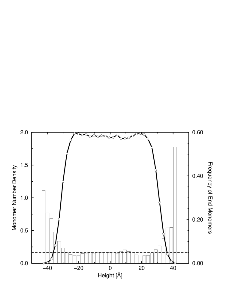
FIG. 7.: Density distribution and chain–end enrichment for the free surface. Shown is the number density of monomers (solid curve, left axis) and the relative frequency of chain–end monomers (bar chart, right axis) in slices parallel to the surface. The polymer system is monodisperse with a chain length of $N=40$. The horizontal dashed line indicates the mean value for chain–ends: $\text{2 ends}/\text{40 monomers}=0.05$.

In Fig. 7, the distribution of the monomer number density vs. the height ($z$) direction (the direction normal to the surfaces) is plotted. As opposed to confined surfaces, no partial crystallization can be observed at free surfaces. Also shown in this figure is the chain–end enrichment. Again in contrast to confined surfaces, we observe the clear tendency for the chain–ends to escape from the bulk. Chain–end monomers require a greater static volume than mid–chain monomers. To reach close packing, they stick to the surface. This is also favoured by reasons of entropy, since the end–monomers possess a higher mobility (they are only constrained by one chemical bond). These arguments, however, do not apply if the surface is pressed by repelling plates. In Fig. 7 one clearly sees the enrichment effect, but an exact quantitative evaluation is out of reach, since if we increase the number of bins next to the surface, the bin width becomes too small to achieve good statistics. The presence of end–monomers of high mobility and the local brush–like structure caused by the chain ends will certainly affect the mechanics of surface disturbances like in an indentation process.

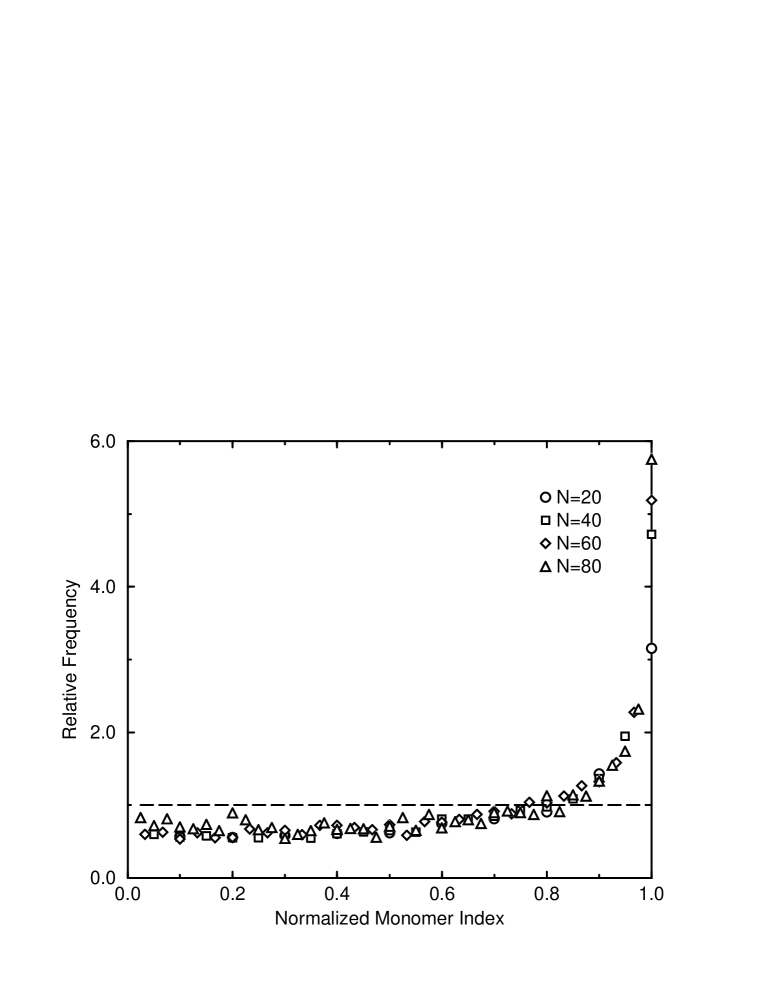
FIG. 8.: The relative frequency of the normalized monomer index at free surfaces for different chain lengths. If all monomers in a chain would appear with the same probability at the surface, the relative frequency would be $1$, independent of the normalized index (dashed horizontal line). However, higher normalized indices are more frequent, a signature of the chain–end enrichment at free surfaces.

A complementary way to analyze chain–end enrichment is to look at the distribution of the normalized monomer index $\tilde{\i}$ which is defined as

$$\tilde{\i}=\frac{|\,i-N/2\,|}{N/2}=\left|\,\frac{2i}{N}-1\,\right|\,.$$ (6)

Mid–chain monomers get the normalized index $0$, for end–monomers it is $1$. Let $n(\tilde{\i})$ be the absolute frequency of the normalized index $\tilde{\i}$ found at the surface and $n_{\text{total}}=\sum_{\tilde{\i}}n(\tilde{\i})$ the total number of all monomers at the surface. These quantities can be determined by dividing the surface into patches, i.e. dividing the whole film into columns. Within each column, we look for the extremal monomers (in a sense, these monomers then define the surface). The same approach is chosen below to sample the surface height function. The relative, chain length independent frequency of $\tilde{\i}$ is then computed according to

$$\tilde{n}(\tilde{\i})=\frac{n(\tilde{\i})}{n_{\text{total}}/(N/2)}=\frac{Nn(\tilde{\i})}{2n_{\text{total}}}\,.$$ (7)

The result for chain lengths $N=20$, $40$, $60$, and $80$ is shown in Fig. 8. If each monomer in the chain would appear with the same probability at the surface, the relative frequency would be $1$, independent of the normalized index (dashed line in the figure). We observe, however, a significant increase in frequency starting with a normalized index of around $0.8$. Moreover, the shape of the curves is very similar for the different chain lengths.

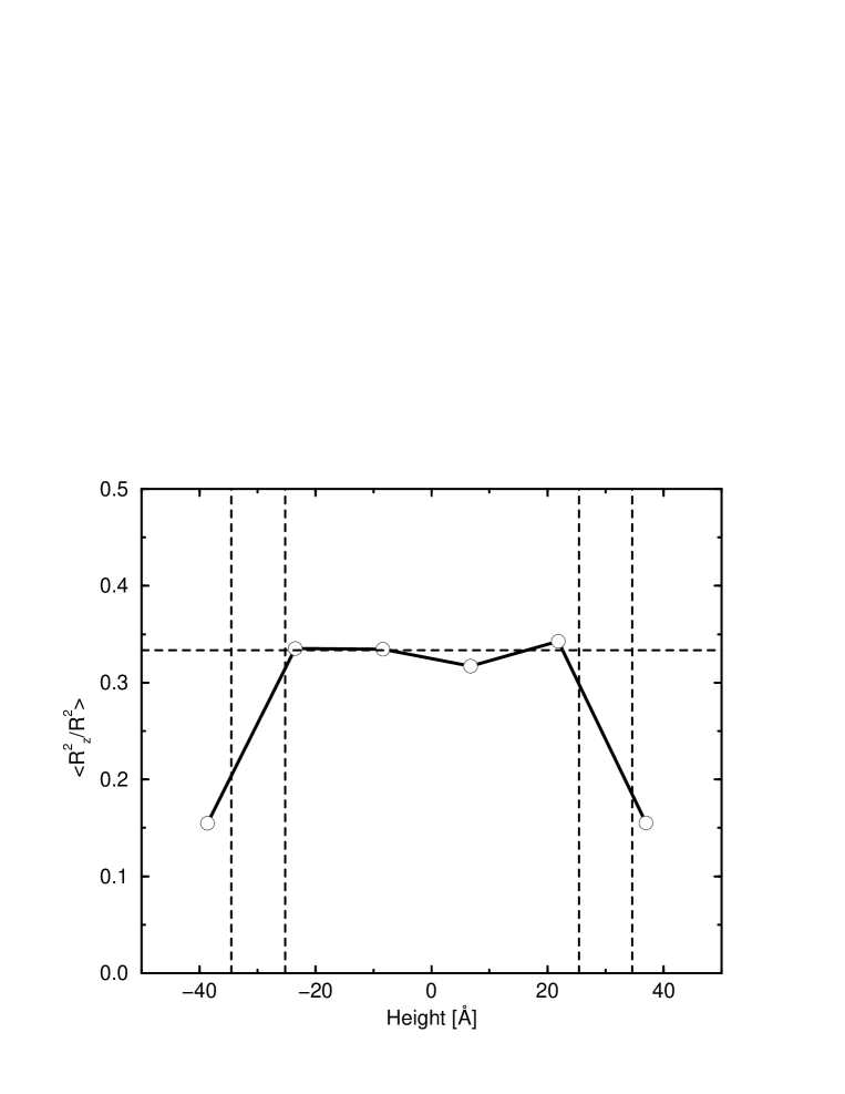
FIG. 9.: The orientation of the end–to–end vector in the free model. Plotted is the mean square value $\langle c^{2}_{\perp}(z)\rangle=\langle{R^{2}_{z}}/{|\vec{R}|^{2}}\rangle$ for the normal–to–surface component after normalization. The mean values are computed in slices parallel to the surfaces at different height. In the bulk, we expect due to equipartition of all directions that $\langle{R^{2}_{z}}/{|\vec{R}|^{2}}\rangle_{\text{bulk}}=1/3$ (horizontal dashed line). The vertical lines mark the extension of the surfaces as given by the 10/90–rule applied to the number density profile in Fig. 7. The average length of the end–to–end vector is found to be 19 Å. This represents a lower bound for the bin width in the figure and severely limits the number of independent data points.

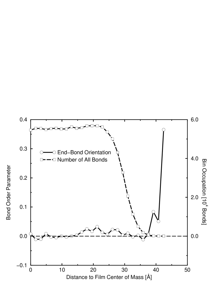
FIG. 10.: The bond order parameter for the chain–end bonds in the free model. The orientation of the end–bonds is plotted vs. their distance from the system’s center of mass (left axis). This involves an average over both surfaces of the film. Good statistics for the end–bonds is difficult to obtain. In chains of length $N=40$, only 5 percent of the monomers are chain–ends. In addition, the number of all bonds becomes very small in the surface region, as can be seen in the bin occupation curve (right axis).

If the chain–ends migrate to the surface, one might suspect some correlation between the orientation of the surface and the chain end–to–end vectors. This is analyzed in Fig. 9. For a given chain, let $\vec{R}_{{\text{i}}}$ denote the monomer positions. Then $\vec{R}=\vec{R}_{\text{N}}-\vec{R}_{\text{1}}$ is the end–to–end vector. As before, the surfaces are parallel to the $xy$–plane. We want to look at the normalized projections of the end–to–end vector normal and parallel to the surface,

$$c^{2}_{\perp}(z)=\frac{R^{2}_{z}}{|\vec{R}|^{2}}\qquad\text{and}\qquad c^{2}_{\parallel}(z)=\frac{R^{2}_{x}+R^{2}_{y}}{|\vec{R}|^{2}}\,.$$ (8)

To place these projection coefficients into bins along the $z$–direction for statistical analysis, we use the mid–point of the end–to–end vector, $z=(R_{\text{N}z}+R_{\text{1}z})/2$. Fig. 9 shows that near the surface, the end–to–end vectors are on average parallel aligned to it. This indicates that both end–monomers of a chain are at the same surface. The alignment, however, does not extend into the plateau region of the density profile. This is an important result, since for thin films, orientational correlations could prevent the formation of a bulk zone at all. Furthermore, the average length of the end–to–end vector in the simulations is 19 Å. Compared to the film height of about 80 Å, there is no separation of scales. A related measure for orientation is the bond order parameter, $b(z)$, defined as

$$b(z)=\frac{\langle b_{z}^{2}\rangle-\frac{1}{2}(\langle b_{x}^{2}\rangle+\langle b_{y}^{2}\rangle)}{\langle|\vec{b}|^{2}\rangle}\,,$$ (9)

where $\vec{b}$ with components $b_{x}$, $b_{y}$, and $b_{z}$ denotes an arbitrary bond vector connecting two monomers. In Fig. 10, the average is over chain–end bonds only. The mean values are computed from a number of statistically independent configurations in bins (slices) of finite width parallel to the film surfaces ($xy$–plane). The bond order parameter is plotted vs. the distance of the bins from the center of mass. In the bulk, we expect isotropic behaviour, yielding $b=0$. We want to test, whether the chain–end bonds in the vicinity of the surface are oriented perpendicular to it, which means $b_{z}^{2}>b_{x/y}^{2}$ resulting in $b>0$. Indeed, from Fig. 10 we infer that this is the case. However, sufficient statistical data for the orientation of the end–bonds at the surface are difficult to obtain. The reason is that we sample in a region in space where the density is already very low.

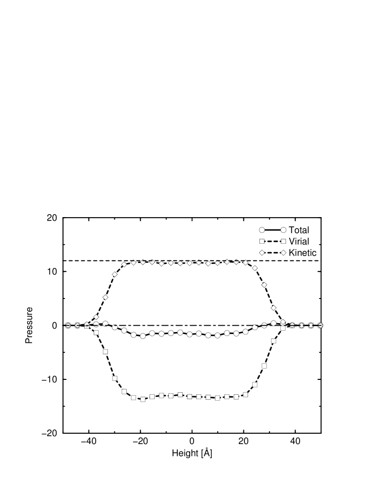
FIG. 11.: The pressure distribution vs. the height direction for the free surface model (pressure in reduced units). The total pressure is the sum of the virial and the kinetic contribution. The dashed horizontal line indicates the expected value for the kinetic (ideal) part: $p^{*}_{\text{ideal}}=\rho^{*}T^{*}\approx 2.0\cdot 6.0=12.0$. The dot–dashed line is the zero pressure line.

Fig. 11 shows the pressure distribution. In effect, a free surface is the interface to a vacuum. This means that the external pressure imposed on the free polymer film is zero. Kinetic and virial contributions should therefore compensate each other. In the figure, the total pressure is slightly less than zero and the system will still contract somewhat during a final relaxation phase that has not been reached in the simulation.

Surface profiles and surface width

In this section, we are concerned with possible analytical fits for surface profiles and the systematic determination of surface location and width. A first idea is to start from the (number or mass) density profile in Fig. 7 and to look for the points $z_{10}$ and $z_{90}$ where 10 and 90 percent of the bulk density are reached. The surface width is the distance between these two points, $\xi=|\,z_{10}-z_{90}\,|$ and as the surface base point we choose the the midpoint, $z_{0}=(z_{10}+z_{90})/2$. In what follows, this method will be called the “10/90–rule”. A second possibility is to fit the density profile with some suitably parameterized analytic function and to use these parameters to actually characterize the surface. This allows to compare profiles which have been fitted using the same family of functions. An appropriate family is based on the hyperbolic tangent,

$$\rho(z)=\frac{1}{2}\rho_{\text{bulk}}\left(1-\tanh\frac{z-z_{\text{t}0}}{\xi_{\text{t}}}\right)\,,$$ (10)

which is essentially the Fermi function, since $(1/2)(1-\tanh x)=(1+\exp 2x)^{-1}$. The 10/90–rule applied to a $\tanh$–fit yields the relations $z_{\text{t}0}=z_{0}$ and $\xi_{\text{t}}=\xi/\ln(0.9/0.1)\approx 0.46\,\xi$. Such a fit is used in Fig. 14. Another possibility is to use the error function (the probability distribution for the Gaussian normal probability density) for the fit,

$$\rho(z)=\rho_{\text{bulk}}\int_{-\infty}^{z}f(\zeta)\,d\zeta\qquad\text{with}\qquad f(z)=\frac{1}{\sqrt{2\pi}\sigma}\exp\left(-\frac{(z-z_{\text{g}0})^{2}}{2\sigma^{2}}\right)\,.$$ (11)

The connection to the 10/90–rule is given by $z_{\text{g}0}=z_{0}$ and $\sigma\approx 2.56\,\xi$. Note that these functions also appear in the following paragraph when characterizing the surface by use of a “height function”, but then they enter in a purely statistical context.

FIG. 12.: The free surface profile as obtained by the statistical analysis of the height function. The circles mark the probability to find the highest (or lowest, respectively) monomer of a column at the given height. This probability density comes from the simulation and has been integrated numerically to determine the associated probability distribution function which is marked by the squares. The probability distribution represents the “surface profile” in the height function approach. The solid curves are analytical fits to the data. For the probability, Gaussian normal densities with $\sigma_{\text{L/R}}=2.56\,\xi_{\text{L/R}}$ are used. The surface profile is a properly located and scaled error function. The surface widths ($\xi_{\text{L}}$ and $\xi_{\text{R}}$) and boundaries (dashed lines) as given by the 10/90–rule are also indicated.

Because of their steepness, surface characterization based solely on the flanks of the density profiles is problematic. The profiles must be determined by sampling monomers. If we put more bins onto the flanks, the bin width soon becomes too small for sufficient statistics. The following method offers a complementary approach. We look onto the upper surface from above and divide it – in the simplest case by use of a regular grid – into a number of patches. Within each patch, (which represents a column in the three–dimensional film) we identify the monomer with the highest $z$–coordinate. In this way we obtain a mapping from the patches to a set of height values. We call this mapping the “height function”. For the given set of height values, we determine mean value and standard deviation and compute from them the location and the width of the surface, respectively. To get the result for the lower surface, we have to pick the lowest monomer within each column. The method is related to the surface contour one obtains using a scanning force microscope. A resolution of 1 or 2 Lennard–Jones $\sigma$ for the resolution (distance between grid lines) is found to be appropriate. When we plot the relative frequency of height values found, we obtain a probability density as in Fig. 12 which can be fitted with a Gaussian normal density. Then the corresponding distribution function is determined which represents some average surface profile.

The relation between the height function profile and the monomer number density profile can be derived in the special case that the monomer density assumes its bulk value instantly below the surface. In this case, the finite slopes in the average density profiles stem only from the fact that the surface is rough. The surface is defined by the height function $h(x,y)$ over a domain in the $xy$–plane with base area $A$. For the height coordinate $z$ we obtain the probability density

$$p_{\text{hf}}(z)=\frac{1}{A}\int\!\!\int dx\,dy\,\delta(h(x,y)-z)\,.$$ (12)

The associated distribution function is ($\Theta\,(\,{z}\,)$ is the unit step function)

$$P_{\text{hf}}(z)=\int_{-\infty}^{z}p_{\text{hf}}(\zeta)\,d\zeta=\frac{1}{A}\int\!\!\int dx\,dy\,\Theta(h(x,y)-z)\,.$$ (13)

On the other hand, the mean density at height $z$ is computed by “counting all columns filled with matter”,

$$\rho(z)=\frac{\rho_{\text{bulk}}}{A}\int\!\!\int dx\,dy\,\Theta(h(x,y)-z)\,.$$ (14)

Under the condition mentioned in the beginning, one therefore finds

$$\rho(z)=\rho_{\text{bulk}}P_{\text{hf}}(z)\,.$$ (15)

Of course, this is what one would have guessed knowing that the density reaches its constant bulk value instantly below a surface with zero local thickness. In Fig. 13 the thickness measures obtained from monomer density profiles and height function statistics are compared to each other for different polymer chain lengths. The fit $\xi\sim N^{-1}$ was successful. We find that for longer chains the height function method, based on the statistics over outermost monomers, certainly overestimates the surface width.

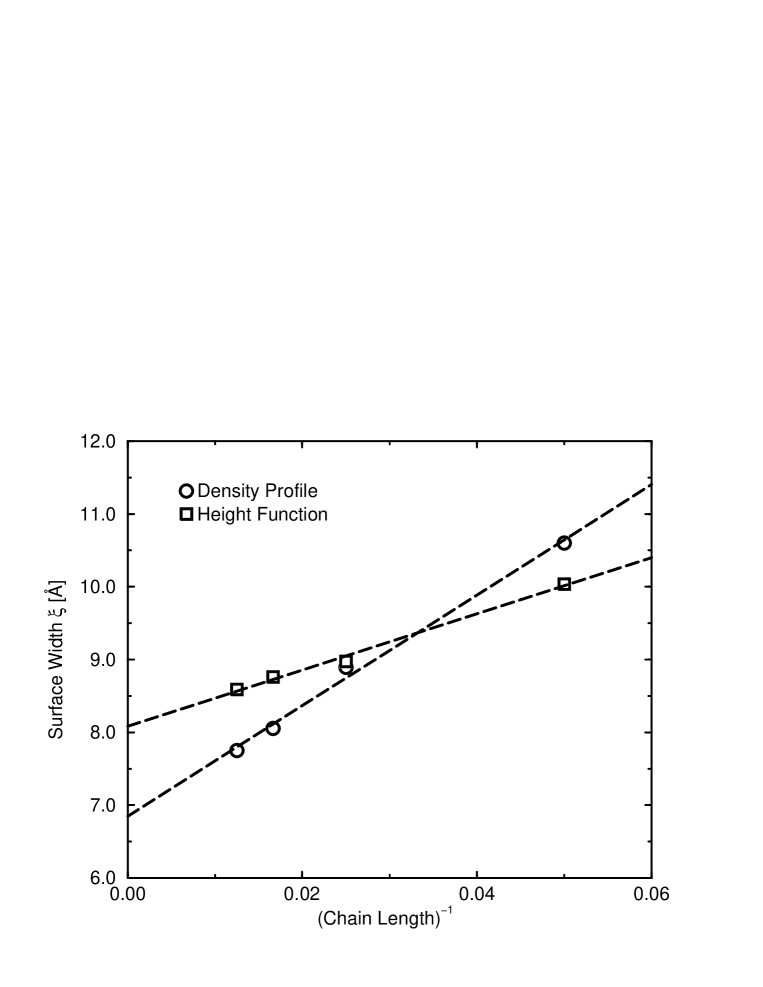
FIG. 13.: The surface width $\xi$ vs. the reciprocal chain length ($N=20$, $40$, $60$, and $80$) in the free model. Slightly different values for $\xi$ are obtained by applying the 10/90–rule either to number density profiles as in Fig. 7 (circles) or to probability distribution profiles based on the height function as in Fig. 12 (squares). The plot suggests a scaling $\xi\sim N^{-1}$. The asymptotic values resulting from linear fits (dashed lines) are $\xi\,(N\to\infty)=6.8\,\text{{\AA}}$ for the density profile and $\xi\,(N\to\infty)=8.1\,\text{{\AA}}$ for the height function method.

Coordination number

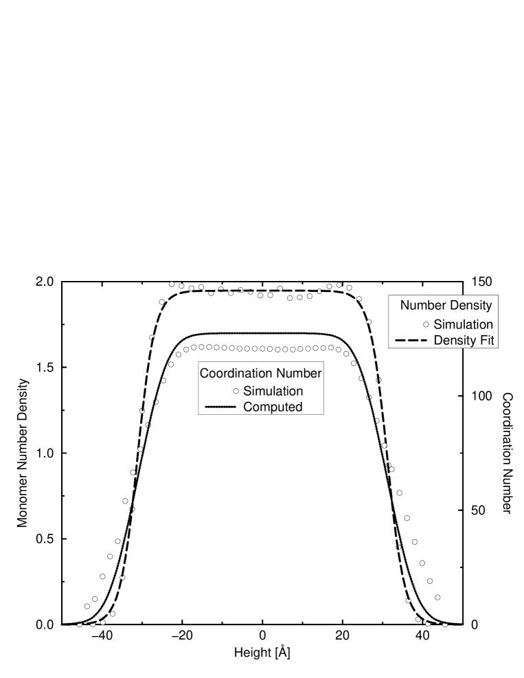
FIG. 14.: Comparison between density profile and coordination number for the free surface model. The simulated density curve is the same as in Fig. 7. For the density fit, a combination of two hyperbolic tangent functions is used. This fit allows a theoretical estimate for the coordination number which is given in the figure, too. In the worst case, the estimate must be determined by a numerical integration, whereas the determination of the coordination numbers from the simulation is more time consumptive. Over all sample configurations, a double loop must be run, since for each monomer we have to count all its interaction partners. Note that the measured coordination number curve is even broader than the theoretical one.

In connection with amorphous materials, the coordination number of a given particle is the number of all its partners involved in van–der–Waals (Lennard–Jones) interactions. From the simulations, this number can simply be determined by counting all the monomers in the interaction range (a sphere of radius $2.5$ Lennard–Jones $\sigma$) of a given monomer (monomers in the same chain do count except they take part in bond length, bond angle, or torsion interactions). Again we assume homogeneity in the lateral ($x$ and $y$) directions, associate with every coordination number the coordinates of its monomer, and set up the distribution of the average coordination number vs. the height ($z$) direction. The result is shown in Fig. 14. A theoretical estimate for the coordination number distribution $c(z)$ must be based on the monomer number density profile $\rho(z)$. Geometric relations then yield the convolution type integral

$$c(z)={\displaystyle\int_{{z}-{\sigma}}^{{z}+{\sigma}}}{\rho}(\,{\zeta}\,)\,{\pi}\,\left(\!\,{\sigma}^{2}-(\,{r}-{\zeta}\,)^{2}\,\!\right)\,{d}{\zeta}\,.$$ (16)

For the monomer density profile, $\rho(z)$, we use the ansatz

$$\rho(z)=\rho_{\text{bulk}}\left[\Theta\,(\,-{z}\,)\,\left(\!\,1+{\rm tanh}\left(\!\,{\displaystyle\frac{z+z_{\text{tL}}}{\xi_{\text{tL}}}}\,\!\right)\,\!\right)+\Theta\,(\,{z}\,)\,\left(\!\,1-{\rm tanh}\left(\!\,{\displaystyle\frac{z-z_{\text{tR}}}{\xi_{\text{tL}}}}\,\!\right)\,\!\right)\right]$$ (17)

with the parameters $\sigma=9.8{\,\text{\AA}}$, $\rho_{\text{bulk}}=1.947$, $z_{\text{tL}}=31.16{\,\text{\AA}}$, $z_{\text{tR}}=31.16{\,\text{\AA}}$, $\xi_{\text{tL}}=4.32{\,\text{\AA}}$, and $\xi_{\text{tR}}=4.32{\,\text{\AA}}$. This results in the computed curve for the coordination number in Fig. 14. The discrepancy in the plateau value derives from the fact that in the estimate we implicitly also count the neighbor monomers in the chain (which should be neglected, see above). As expected, the flanks of the coordination number distribution are broader than the flanks of the density profile. This means that in the interaction picture, the surface region is further extended than according to the local density criterion.

Conclusion and outlook

We have presented two methods to prepare amorphous polymer surfaces in molecular dynamics simulations with united atom models for the polymer chains. The ideas involved can easily be transfered to both more detailed models (which, as one extreme, explicitly treat each atom in a monomer, or, like the ellipsoidal model [14] for BPA–PC, extend the united atom model by considering the geometric shape of a monomer) and more coarse–grained polymer models. The use of classical molecular dynamics algorithms is not mandatory. Monte–Carlo and Hybrid Monte–Carlo techniques can be employed as well and the inclusion of stochastic Langevin forces (Brownian motion) is straightforward (and, in fact, implemented in our simulation program). The present work is also a further step in extending the versatility of The Materials Explorer, a continuously growing, integrated software tool for the simulation, visualization, and quantitative analysis of engineering materials [15]. The work presented here will allow us to analyze our simulations on nano–mechanical surface indentation processes [5] in which we prepare a surface using one of the methods discussed above. After that, the impact of the indentation tool causes local disturbations and the deviation of the certain observables from their equilibrium values gives us information about the surface resistance and friction properties. Related to the indentation processes are simulations on thin film bending [6]. A tool, which is more carefully driven as in the indentation experiment, causes non–local, large–scale deformations in the polymer film. Again various observables (density distribution, orientation of the chain molecules) deviate from their equilibrium values and have to be analyzed.

REFERENCES

- [1] D. B. Bogy, C. J. Lu, Z. G. Jiang, and T. Miyamoto, Z. f. Angew. Math. und Phys. 46, 483 (1995); E. Hamada and R. Kaneko, J. Phys. D 25, A53 (1992).
- [2] R. T. Spurr, Wear 79, 301 (1982); T. A. Stolarski, Tribology in Machine Design (Heinemann Newnes, 1990); I. M. Hutchings, Tribology (Edward Arnold, London, 1992); J. R. Cooper, D. Dowson, and J. Fisher, Wear 162, 378 (1993).
- [3] D. W. Heermann, Computer Simulation Methods in Theoretical Physics (Springer–Verlag, Heidelberg, 1986).
- [4] T. K. Xia, J. Ouyang, M. W. Ribarsky, and U. Landman, Phys. Rev. Lett. 69, 1967 (1992); W. D. Luedtke and U. Landman, Comp. Mat. Sci. 1, 1 (1992).
- [5] A. Linke, Th. Hapke and D. W. Heermann (to be published).
- [6] G. Pätzold, Th. Hapke, A. Linke, and D. W. Heermann (to be published).
- [7] M. P. Allen and D. J. Tildesley, Computer Simulation of Liquids (Clarendon Press, Oxford, 1987); D. Rigby and R. J. Roe, J. Chem. Phys. 87, 7285 (1987); Th. Hapke, Simulation mikromechanischer Eigenschaften von amorphen makromolekularen Gläsern am Beispiel von Polyethylen, Diplomarbeit am Institut für Theoretische Physik der Universität Heidelberg, 1995.
- [8] W. Paul, D. Y. Yoon, and G. D. Smith, J. Chem. Phys. 103, 1702 (1995).
- [9] W. Paul, K. Binder, D. W. Heermann, and K. Kremer, J. Chem. Phys. 95, 7726 (1991).
- [10] P. K. Brazhnik, K. F. Freed and H. Tang, J. Chem. Phys. 101, 9143 (1994).
- [11] Y. Rouault, B. Dünweg, J. Baschnagel, and K. Binder, Polymer 37, 297 (1996).
- [12] J. H. J. Van Opheusden, J. M. M. De Nijs, and F. W. Wiegel, Physica A 134, 59 (1985).
- [13] J. S. Wang and K. Binder, J. Phys. 1, 1583 (1991).
- [14] K. M. Zimmer and D. W. Heermann, J. Computer–Aided Materials Design 2, 1 (1995); K. M. Zimmer, A. Linke, D. W. Heermann, and J. Batoulis (to be published).
- [15] A. Linke, D. W. Heermann, and Ch. Münkel, in Proceedings of the HPCN 1995 (Lect. Notes in Comp. Science, Springer–Verlag, Heidelberg, 1995), p. 928.