On Metal–Insulator Transitions due to Self–Doping

Abstract

We investigate the influence of an unoccupied band on the transport properties of a strongly correlated electron system. For that purpose, additional orbitals are coupled to a Hubbard model via hybridization. The filling is one electron per site. Depending on the position of the additional band, both, a metal–to–insulator and an insulator–to–metal transition occur with increasing hybridization. The latter transition from a Mott insulator into a metal via “self–doping” was recently proposed to explain the low carrier concentration in $\rm Yb_{4}As_{3}$. We suggest a restrictive parameter regime for this transition making use of exact results in various limits. The predicted absence of the self–doping transition for nested Fermi surfaces is confirmed by means of an unrestricted Hartree–Fock approximation and an exact diagonalization study in one dimension. In the general case metal–insulator phase diagrams are obtained within the slave–boson mean–field and the alloy–analog approximation.

I Introduction

One of the most remarkable examples of the failure of the independent–electron approximation is the existence of so–called Mott–Hubbard insulators. The early transition oxides like $\rm LaVO_{3}$, $\rm LaTiO_{3}$, $\rm V_{2}O_{3}$, $\rm Ti_{2}O_{3}$ or $\rm Cr_{2}O_{3}$ show an insulating behaviour, although they contain partially filled $d$ bands. The reason is the strong Coulomb repulsion of the $d$ electrons, which hinders them from moving freely. A simple model to describe the situation is the Hubbard Hamiltonian with one electron per site [1]:

$$H\,=\,\sum_{i,j,\sigma}t_{ij}\,f_{i\sigma}^{\,\dagger}f_{j\sigma}+U\sum_{i}n_{i\uparrow}n_{i\downarrow}.$$ (1)

Electrons can hop from one site $i$ to another $j$ via the hopping–matrix element $t_{ij}$. Whenever two electrons (of opposite spins) occupy the same site, they repel each other with an interaction energy $U$.

To obtain insulating behaviour (implying a vanishing dc conductivity at zero temperature) an energy gap for charge excitations is required. The existence of a conductivity gap can be inferred from the spectral density of states $\rho(\omega)$. Obviously, for large Coulomb repulsion and half–filling there is a gap of order $U$. The transition from a metallic ($U=0$) to an insulating ($U$ large) state is still subject of intensive investigations [2]. For general lattices (without special symmetry properties) there is reason to believe that the transition takes place at a finite value $U=U_{c}\not=0$ [2, 3, 4].

The Hubbard model deals with one orbital per site and ignores any additional bands which might be present. As was first pointed out by Zaanen, Sawatzky and Allen [5] this is not sufficient for a classification of the transition metal oxides. The following Hamiltonian represents a natural extension of the Hubbard model by including one additional spin–orbital with creation operators $c_{i\sigma}^{\,\dagger}$ for each site $i$:

$$H = -\Delta\sum_{i\sigma}n_{i\sigma}^{\,f}+\sum_{i,j,\sigma}t_{ij}\,f_{i\sigma}^{\,\dagger}f_{j\sigma}+U\sum_{i}n_{i\uparrow}^{\,f}n_{i\downarrow}^{\,f}$$ (3)

$${}+\sum_{i,j,\sigma}\tilde{t}_{ij}\,c_{i\sigma}^{\,\dagger}c_{j\sigma}+V\sum_{i\sigma}\left(f_{i\sigma}^{\,\dagger}c_{i\sigma}+{\rm h.c.}\right).$$

In the following we will refer sometimes to the additional orbital as a ligand orbital implying that it may belong to a ligand atom. Note, that the on–site energy of the ligand orbitals has been set equal to zero. Therefore the ligand orbitals are higher in energy than the $f$ orbitals ($\Delta\geq 0$). The system is assumed to be quarter–filled, i.e., with one electron (or hole) per site.

Zaanen et al. [5] employed a single–impurity approach to derive a phase diagram for the transition–metal compounds. Thereby the transition–metal atoms are taken to be independent. This implies a neglect of the hopping term $t_{ij}$ in (3). Moreover, indirect hopping processes between the $f$ orbitals via the $c$ orbitals are excluded. The calculated band gaps in the density of states then approximately scale with the hybridization $V$. Beside the Mott–Hubbard regime, where the gap is proportional to $U$, a second region with a gap proportional to $\Delta$ was identified. For this phase the term charge–transfer insulator is used. As a consequence of the single–impurity approach a metallic state was predicted when the transition–metal level lies within the free electron band of the ligand host. In contrast, a hybridization gap may be obtained when taking into account coherence effects of the transition–metal atoms. Nimkar et al. [6] and Sarma and Barman [7] called the insulating phase due to a hybridization gap a covalent insulator and derived the corresponding region of the phase diagram. The special feature of a covalent insulator is, that it undergoes an insulator–to–metal transition with decreasing hybridization. The gap does not scale with $V$. $\rm LnNiO_{3}$ (with Ln a rare earth ion other than La) and $\rm NiS$ are believed to belong to this class [6]. They can be driven into a metallic state without a symmetry lowering structural transition by varying pressure or temperature.

If we do not neglect the hopping term $t_{ij}$ in (3), we can also imagine the opposite taking place, i.e., an insulator–to–metal transition with increasing hybridization. Electrons hopping into ligand levels create holes in the Hubbard system, which may move and contribute to the conductivity. A mechanism of this kind was recently proposed for the rare–earth compound $\rm Yb_{4}As_{3}$ [8]. Such an insulator–to–metal transition due to “self–doping” would be an interesting new possibility for forming metals with low carrier concentration. Moreover, like the Mott–Hubbard insulator, it cannot be understood within an independent electron picture.

To investigate in more detail the influence of an additional band on the transport properties of a strongly correlated electron system we suggest the following model:

$$H = -\Delta\sum_{i,\sigma}n_{i\sigma}^{\,f}+\sum_{i,j,\sigma}t_{ij}\,f_{i\sigma}^{\,\dagger}f_{j\sigma}+U\sum_{i}n_{i\uparrow}^{\,f}n_{i\downarrow}^{\,f}$$ (5)

$${}+V\sum_{i,\sigma}\left(f_{i\sigma}^{\,\dagger}c_{i\sigma}+{\rm h.c.}\right).$$

Again, the system is assumed to be quarter–filled, i.e., it has one electron per site. The Coulomb repulsion is chosen to be greater than the critical value $U_{c}$ of the Hubbard system. Therefore we will call the model a self–doped Mott system (SMS) in the following. In comparison to the Hamiltonian (3) we have neglected the hopping $\tilde{t}_{ij}$ between the ligand orbitals. For realistic situations this approximation is not justified, neither for rare–earth nor for transition–metal compounds. Note, that in systems like $\rm Yb_{4}As_{3}$ the widths of the correlated and uncorrelated bands are equal ($t_{ij}=\tilde{t}_{ij}$). The Hamiltonian (5) should be regarded as a basic model containing the necessary terms for the self–doping mechanism. Moreover, whenever we have included the hopping term $\tilde{t}_{ij}$ we found no change in the general behaviour. We will come back to this point later.

In this paper we report first results of an investigation of the system described by (5). In Section II we illustrate in a transparent way some model properties. We discuss exact solutions in the limit of zero bandwidth and of infinite hybridization. Concerning the metal–insulator transition in the Hubbard model two different situations have to be distinguished. In the case of a nested Fermi surface the Hubbard model at half filling is an insulator for any $U>0$ [9]. We investigate this case for the SMS by means of an unrestricted Hartree–Fock approximation [10] and present the results in Section III. Additionally the one–dimensional case is studied by exactly diagonalizing a finite system. Two early approaches have dominated the discussion about the Mott–Hubbard transition for general lattices without nesting: (i) the Brinkman–Rice approach [11], which can be formally derived by using slave boson methods [12], and (ii) the alloy analogy, which is contained in the first part of the well–known Hubbard III paper [13]. We apply these approximation schemes to our model and present the results in Section IV. Finally, Section V contains a short summary and outlook.

II The model

In the case of vanishing hybridization the SMS reduces to a Hubbard model with a separated ligand level. In the first column of Fig. 1 we sketch the corresponding density of states. For $U>U_{c}$ three different regions exist (indicated by (2), (3) and (4) in that figure):

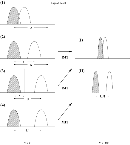
FIG. 1.: Schematic plot of the density of state $\rho(\omega)$ for the SMS in the extreme limits of vanishing and infinite hybridization. The occupied (electron–removal) part is hatched. With IMT and MIT we indicate an insulator–to–metal and a metal–to–insulator transition, respectively. Different parameter regions are shown (see text).

• Mott–Hubbard insulator: $U<\Delta$. When adding one electron to the system the lowest energy states contain an additional double occupied $f$ orbital. The gap is of order $U$ (Fig. 1, (2)).

• Charge transfer insulator: $U>\Delta$. An additional electron avoids the Coulomb repulsion felt in the $f$ subsystem and prefers to occupy the ligand orbital. The energy scale of the gap is set by $\Delta$ (Fig. 1, (3)).

• Due to the hopping term $t_{ij}$ the lower and upper Hubbard bands possess a finite bandwidth $W(U)$. The ground state of the SMS contains occupied ligand orbitals if the gain of kinetic energy due to holes in the Hubbard subsystem overcomes the transfer energy: $\Delta<W$. Adding or removing one electron changes the energy only infinitesimally. The system is metallic (Fig. 1, (4)).

We turn now to the case of infinite hybridization. For $V\gg\Delta$ it is convenient to use a basis in which the hybridization term is diagonal. Introducing:

$$a_{i\sigma}=\frac{1}{\sqrt{2}}\left(f_{i\sigma}+c_{i\sigma}\right)\;,\;b_{i\sigma}=\frac{1}{\sqrt{2}}\left(f_{i\sigma}-c_{i\sigma}\right),$$ (6)

we obtain for the Hamiltonian (5):

$$H=H_{a}+H_{b}+H_{ab}$$ (7)

with:

$$H_{a} = \left(-\frac{\Delta}{2}+V\right)\,\sum_{i,\sigma}a_{i\sigma}^{\,\dagger}a_{i\sigma}+\frac{1}{2}\,\sum_{i,j,\sigma}t_{ij}\,a_{i\sigma}^{\,\dagger}a_{j\sigma}$$

$${}+\frac{U}{4}\,\sum_{i}n_{i\uparrow}^{a}n_{i\downarrow}^{a}$$

$$H_{b} = \left(-\frac{\Delta}{2}-V\right)\,\sum_{i,\sigma}b_{i\sigma}^{\,\dagger}b_{i\sigma}+\frac{1}{2}\,\sum_{i,j,\sigma}t_{ij}\,b_{i\sigma}^{\,\dagger}b_{j\sigma}$$

$${}+\frac{U}{4}\,\sum_{i}n_{i\uparrow}^{b}n_{i\downarrow}^{b}$$

$$H_{ab} = -\frac{\Delta}{2}\,\sum_{i,\sigma}\left(a_{i\sigma}^{\,\dagger}b_{i\sigma}+{\rm h.c.}\right)+\,\frac{1}{2}\,\sum_{i,j,\sigma}t_{ij}\left(a_{i\sigma}^{\,\dagger}b_{j\sigma}+{\rm h.c.}\right)$$

$$-\,\frac{U}{4}\sum_{i}\{n_{i\uparrow}^{a}n_{i\downarrow}^{a}+n_{i\uparrow}^{b}n_{i\downarrow}^{b}$$

$$-\left.\left.\left.\left.\left.\left.\!\!\!\!\left(a_{i\uparrow}^{\,\dagger}+b_{i\uparrow}^{\,\dagger}\right)\right(a_{i\uparrow}+b_{i\uparrow}\right)\right(a_{i\downarrow}^{\,\dagger}+b_{i\downarrow}^{\,\dagger}\right)\right(a_{i\downarrow}+b_{i\downarrow}\right)\}.$$

For $V=\infty$ the $a$ orbitals remain empty and we can restrict ourselves to the part $H_{b}$. The SMS reduces to a Hubbard model with a hopping matrix $t_{ij}/2$ and a Coulomb repulsion $U/4$. The result is easily understood. When the two orbitals at a given site hybridize strongly with each other, the eigenstates are given by the bonding $b$ and antibonding $a$ linear combinations. Only the $b$ orbitals are populated to which the original $f$ orbitals contribute by one half. The Coulomb repulsion felt by two electrons occupying one $b$ orbital is reduced to a quarter and the hopping between two $b$ orbitals is reduced to one half. The trivial but important observation is, that the Coulomb repulsion is stronger reduced than the hopping. Since only the relation between these two quantities is important, the SMS describes for $U/2<U_{c}$ a metal and for $U/2>U_{c}$ an insulator ($V=\infty$). This is indicated in the second column of Fig. 1 by (I) and (II), respectively.

Having discussed the extreme limits, two transitions seem to be possible when changing the hybridization $V$ from zero to infinity: For $\Delta<W(U)$, $U>2U_{c}$ a metal–to–insulator and for $\Delta>W(U)$, $U_{c}<U<2U_{c}$ an insulator–to–metal transition should take place with increasing $V$. Here $W(U)$ is the effective band width of the lower Hubbard band. The two possibilities correspond to the aforementioned covalent insulator and a self–doped metallic state, respectively. It is worthwhile to note that the second scenario is realized only if $U_{c}>0$, i.e., for a finite value of the critical Coulomb repulsion $U_{c}$ in the corresponding Hubbard model.

In order to gain better insight into the behaviour of the system for finite hybridization we have considered the zero bandwidth limit of the SMS:

$$H\,=\,-\Delta\sum_{\sigma}n_{\sigma}^{\,f}+U\,n_{\uparrow}^{\,f}n_{\downarrow}^{\,f}+V\sum_{\sigma}\left(f_{\sigma}^{\,\dagger}c_{\sigma}+{\rm h.c.}\right).$$ (8)

The Hamiltonian is easily diagonalized, yielding the eigenvalues $E_{m}^{(n)}$ and eigenstates $\left|m^{(n)}\,\right\rangle$ for $n$ electrons ($n=1,2,3$). The $f$ density of states is given by:

$$\rho^{\,f}(\omega) = \sum_{m,i,\sigma}\{\,\left|\left\langle\,m^{(N_{e}+1)}\left|f_{i\sigma}^{\,\dagger}\right|0^{(N_{e})}\right\rangle\right|^{2}$$ (12)

$${}\;\;\;\;\;\;\;\;\,\;\;\;\;\;\times\delta(\omega+E_{0}^{(N_{e})}-E_{m}^{(N_{e}+1)})\,$$

$$\;\;\;\;\;\;+\left|\left\langle\,m^{(N_{e}-1)}\left|f_{i\sigma}\right|0^{(N_{e})}\right\rangle\right|^{2}$$

$$\;\;\;\;\;\;\;\;\,\;\;\;\;\;\times\delta(\omega+E_{m}^{(N_{e}-1)}-E_{0}^{(N_{e})})\}.$$

Here $N_{e}=1$ and the sum is only over one site. Furthermore, $\mid\!0^{(N_{e})}\rangle$ denotes the ground state. A similar expression holds for the density of states of the $c$ electrons. The total one is given by $\rho(\omega)=\rho^{f}(\omega)+\rho^{c}(\omega)$.

In Fig. 2 we show the results of the diagonalization. Plotted are the positions of the poles and their weights in the density of states. For small hybridization we can clearly identify the lower and upper Hubbard peaks, as well as the peaks caused by adding one electron to the ligand orbital situated at $\omega\approx 0$ ($f^{\,1}c^{\,0}\rightarrow f^{\,1}c^{\,1}$) and $\omega\approx\Delta$ ($f^{\,1}c^{\,0}\rightarrow f^{\,0}c^{\,2}$). Due to the different effect of the hybridization on a singlet and a triplet state the $f^{\,1}c^{\,1}$–peak splits up. As a result weight is pushed towards the lower Hubbard peak. We stress that there is no direct weight transfer between the lower and upper Hubbard peak. Instead, the weight of the lower Hubbard peak is always equal to unity. Thus a simple self–doping picture which predicts a metallic state for an infinitesimal small hybridization $V$ does not hold true in that case. Note, that the gap $E_{\rm gap}=E_{0}^{(2)}+E_{0}^{(0)}-2E_{0}^{(1)}$ between the occupied and unoccupied part of the spectra continously decreases from $E_{\rm gap}=\Delta$ to $E_{\rm gap}\approx U/4$. When the full Hamiltonian is used the peaks will mark the position of centers of bands. An overlap of the bands accompanied by an insulator–to–metal transition is expected, when the hybridization $V$ exceeds a critical value $V_{c}$.

FIG. 2.: Schematic representation of the excitations from the ground state of the SMS in the zero bandwidth limit on adding and removing an electron. Indicated are the weights in the spectral density. Various values of the hybridization are used ($\Delta=2$, $U=4$).

III Nested Fermi surface

We turn now to a treatment of the full Hamiltonian (5). In this section we consider lattice symmetries and hopping matrices which lead to a nested Fermi surface. The critical Coulomb repulsion in the corresponding Hubbard model vanishes. In one spatial dimension this is the general behaviour. The dimension $d=1$ allows for an exact diagonalization study. Higher dimensions are treated within the unrestricted Hartree–Fock approximation, which getting exact in the limit $U\rightarrow 0$ and in the atomic limit $U=\infty$. Note, that in the case of $U_{c}=0$ small Coulomb repulsions are the most interesting. After the discussion of Section II the behaviour for values $U$ $\stackrel{{\scriptstyle\scriptstyle>}}{{\scriptstyle\sim}}$ $U_{c}$ should be representative also for all $U>U_{c}$.

A Unrestrictive Hartree–Fock approximation

We assume in the following a bipartite lattice. Additional lattice symmetry properties enter the calculation only via the band dispersion $\epsilon_{\vec{k}}$, which is the Fourier transform of the hopping matrix

$$t_{ij}=\frac{1}{N}\,\sum_{\vec{k}}\epsilon_{\vec{k}}\,e^{i\,\vec{k}\,(\vec{r}_{i}-\vec{r}_{j})}.$$ (13)

Here $N$ is the number of sites in the lattice. It is convenient to introduce the density of states of free particles:

$$\rho_{0}(\omega)=\frac{1}{N}\,\sum_{\vec{k}}\delta(\omega-\epsilon_{\vec{k}}).$$ (14)

In the calculations presented in this paper it suffices to specify $\rho_{o}(\omega)$ instead of the lattice structure and the hopping matrix elements. In order to proceed analytically as far as possible, we will use in the following a rectangular density of states:

$$\rho_{o}(\omega)=\frac{1}{2W}\,\Theta(W-\omega)\,\Theta(W+\omega),$$ (15)

where $\Theta(\omega)$ is the step function. This choice maintains the antiferromagnetic instability for arbitrarily small values of $U$ and represents the situation of a nested Fermi surface.

In the mean–field approach the interaction term of the Hamiltonian (5) is linearized, i.e.,

$$n_{i\uparrow}^{f}n_{i\downarrow}^{f}\,\longrightarrow\,n_{i\uparrow}^{f}\langle\,n_{i\downarrow}^{f}\,\rangle+\langle\,n_{i\uparrow}^{f}\,\rangle n_{i\downarrow}^{f}-\langle\,n_{i\uparrow}^{f}\,\rangle\langle\,n_{i\downarrow}^{f}\,\rangle.$$ (16)

The electrons interact via a molecular field. Depending on the anticipated symmetry of the ground state, different ansatzs for the expectation values $\langle\,n_{i\sigma}^{\,f}\,\rangle$ are made. In the case of antiferromagnetic order two sublattices $A$ and $B$ are introduced. The following ground states are considered
$\bullet$ paramagnetic : $\langle\,n_{i\uparrow}^{f}\,\rangle=\frac{1}{2}\,(1-\delta)=\langle\,n_{i\downarrow}^{f}\,\rangle$, $\bullet$ ferromagnetic : $\langle\,n_{i\uparrow}^{f}\,\rangle=\frac{1}{2}\,(1-\delta+m)$, $\langle\,n_{i\downarrow}^{f}\,\rangle=\frac{1}{2}\,(1-\delta-m)$, $\bullet$ antiferromagnetic : $\langle\,n_{i\uparrow}^{f\,A}\,\rangle=\frac{1}{2}\,(1-\delta+m)=\langle\,n_{i\downarrow}^{f\,B}\,\rangle$, $\langle\,n_{i\downarrow}^{f\,A}\,\rangle=\frac{1}{2}\,(1-\delta-m)=\langle\,n_{i\uparrow}^{f\,B}\,\rangle$ .
These are the main states in the phase diagram of the doped Hubbard model calculated by Penn [14]. We indicate now the construction of the phase diagram for the SMS. Following Langer et al. [15] we solve the equation of motion for the one–particle Green’s function $\langle\langle\,f_{\vec{k}\sigma}\,;\,f_{\vec{k}\sigma}^{\,\dagger}\,\rangle\rangle\!{\atop\omega}$ and $\langle\langle\,c_{\vec{k}\sigma}\,;\,c_{\vec{k}\sigma}^{\,\dagger}\,\rangle\rangle\!{\atop\omega}$. From the imaginary part the spectral densities $\rho_{\vec{k}\sigma}^{f}(\omega)$ and $\rho_{\vec{k}\sigma}^{c}(\omega)$ are obtained. For zero temperature the magnetization $m$ and the self–doping $\delta$ are given by the solution of:

$$\frac{1}{N}\,\sum_{\vec{k},\sigma}\,\int\limits_{-\infty}^{\mu}\left(\rho_{\vec{k}\sigma}^{f}(\omega)+\rho_{\vec{k}\sigma}^{c}(\omega)\right)\,d\omega = 1$$ (17)

$$\frac{1}{N}\,\sum_{\vec{k}}\,\int\limits_{-\infty}^{\mu}\rho_{\vec{k}\uparrow}^{f}(\omega)\,d\omega = \frac{1}{2}\left(1-\delta+m\right)$$ (18)

$$\frac{1}{N}\,\sum_{\vec{k}}\,\int\limits_{-\infty}^{\mu}\rho_{\vec{k}\downarrow}^{f}(\omega)\,d\omega = \frac{1}{2}\left(1-\delta-m\right)\,,$$ (19)

where we have introduced the chemical potential $\mu$. The equations (17) are solved numerically by iteration using for $\rho_{0}(\omega)$ a rectangular form. Knowing the parameters $m$, $\delta$ and $\mu$ for the ground state of a given symmetry the energies of the various states are calculated. The state with the lowest energy is the true ground state and determines the spectrum.

First we discuss the result for $V=0$. In the antiferromagnetic phase the model corresponds to an insulator. The corresponding spectral density is the one indicated in Fig. 1, (2) and (3). For $\Delta>W$ the ground state is antiferromagnetic for all $U$. This phase can also be present if $\Delta<W$. In particular we obtain an insulating antiferromagnetic solution for small $U<\Delta$ up to $\Delta=0$. This reflects the fact that the ground state does not contain occupied $c$ orbitals. The $f$ subsystem is undoped.

We now turn to the results for finite hybridization. Our calculations show that the insulating phases survive, when the hybridization $V$ is changed from zero to a finite value. In the limit $V\rightarrow\infty$ the ground state is an antiferromagnetic insulator for all values of $\Delta$ and $U$. No insulator–to–metal transition takes place. In Section II we have argued that this behaviour requires a vanishing critical Coulomb repulsion for the Hubbard model. Therefore the obtained result confirms our prediction.

As mentioned before, in the limit $V\rightarrow\infty$ the system is always insulating. This finding implies a metal–to–insulator transition due to the opening of a hybridization gap in a certain parameter regime. We have identified a regime with $V_{c}=0$ and one with a finite critical value of the hybridization for the transition to an insulator. Details will be presented elsewhere. Here we characterize the two regimes only roughly by $\Delta\leq U\leq 2W$ and $2W\leq U\leq 4W$, respectively ($\Delta\ll W$).

B Exact diagonalization in one dimension

In one spatial dimension the critical Coulomb repulsion $U_{c}$ of the Hubbard model with nearest neighbour hopping vanishes. The model should be insulating for all values of $U$ and $V$ ( $\Delta>W$). Extending the Hamiltonian (5) to (3), i.e., including a hopping term between different $c$ orbitals, does not change the result qualitatively. In the limit $V\rightarrow\infty$ the Hamiltonian (3) reduces to a single band Hubbard model with a Coulomb repulsion $U/4$ and hopping matrix elements $(t_{ij}+\tilde{t}_{ij})/2$. A self-doping transition can only be expected within the parameter regime $\Delta>W(U)+\tilde{W}$ and $U_{c}<U<2\,(1+\tilde{W}/W)\,U_{c}$. With $W$ and $\tilde{W}$ we denote half of the bandwidth of the $f$ and the $c$ bands, respectively. Here the conditions on $U$ are less restrictive as before.

To verify the prediction we have performed an exact diagonalization of the Hamiltonian (3) on a four site chain. Treating the extended model in this approach is no additional difficulty. Before presenting the results we first indicate the calculations. The one particle excitation spectrum is defined by Eq. (12). The first and second term give the electron addition and electron removal spectrum, respectively. The spectral density $\rho(\omega)$ for small clusters can be obtained by the Lanczos algorithm in form of a continued-fraction [16]. In order to obtain the electron removal spectrum, we start from the vector $\psi_{0}=f_{i\sigma}\,\psi_{0}^{(Ne)}$ and then tridiagonalize the Hamiltonian by the Lanczos method. The positions of the poles and their weights follow from diagonalizing the tridiagonal matrix. The electron addition spectrum is obtained similarly.

FIG. 3.: Evolution of the spectral density of the extended model (3) in one dimension. Results are shown for a four site chain. Periodic and antiperiodic boundary conditions are used. The parameters are given by: $U=4$, $\Delta=2$, $W=0.25$, $\tilde{W}=1.5$. The solid and dashed lines indicate the $f$ and $c$ spectral density, respectively. The vertical line marks the position of the chemical potential. The peaks have been broadened by $\epsilon=0.05$.

Results are shown in Fig. 3. We follow the usual representation and plot the $\delta$–function of equation (12) with a (arbitrary) width $\epsilon=0.05$ $(\delta(\omega-\omega_{\rm pol})\rightarrow-\frac{1}{\pi}\,{\rm Im}\left(\frac{1}{\omega-\omega_{\rm pol}+i\epsilon}\right))$. A pseudo–gap seems to exist between the electron removal and the electron addition spectra. This is caused by the broadening. In all our calculations there is clearly a gap between the occupied and unoccupied part of the spectrum. The energy regime without weight is much larger than the typical distance between the poles. To summarize, the Lanczos calculations predict an insulator for the extended model $(\Delta>W+\tilde{W})$ in one spatial dimension. Thus in the extended model the self-doping transition is restricted to a limited parameter regime. This behaviour is similar to the one of the SMS.

IV General lattices

In this section we treat the Hamiltonian (5) within (i) the slave–boson mean–field and (ii) the alloy–analog approximation. We restrict ourselves to a paramagnetic ground state. Nevertheless correlation effects are included and both approximations predict a finite critical Coulomb repulsion for the Mott–Hubbard transition. The restriction to a paramagnetic ground state does not allow the resolution of details of the underlying lattice symmetry. The results are therefore interpreted as the behaviour of the SMS on a general lattice. We have excluded here the case of a nested Fermi surface. Again it suffices to specify $\rho_{o}(\omega)$. In the slave–boson approach we will use a rectangular form as before and in the alloy analogy we will choose an elliptical one:

$$\rho_{o}(\omega)=\frac{2}{W^{2}\pi}\,\sqrt{W^{2}-\omega^{2}}.$$ (20)

A Slave–boson mean–field approximation

In the slave–boson approach four bosonic fields are introduced with creation operators $d_{i}^{\,\dagger}$, $s_{i\sigma}^{\,\dagger}$ and $e_{i}^{\,\dagger}$. They correspond to the four possible states of an $f$ orbital, i.e., double occupation, single occupation with spin $\sigma=\pm 1$ and empty state. The following constrains ensure that only the physically relevant part of the enlarged Hilbert space is considered

$$e_{i}^{\,\dagger}e_{i}+s_{i\uparrow}^{\,\dagger}s_{i\uparrow}+s_{i\downarrow}^{\,\dagger}s_{i\downarrow}+d_{i}^{\,\dagger}d_{i} = 1$$ (21)

$$s_{i\sigma}^{\,\dagger}s_{i\sigma}+d_{i}^{\,\dagger}d_{i} = f_{i\sigma}^{\,\dagger}f_{i\sigma}.$$ (22)

Having introduced the bosonic fields the Hamiltonian (5) projected onto the physical subspace can be expressed in the form

$$H = -\Delta\sum_{i,\sigma}f_{i\sigma}^{\,\dagger}f_{i\sigma}+\sum_{i,j,\sigma}t_{ij}\,z_{i\sigma}^{\,\dagger}f_{i\sigma}^{\,\dagger}f_{j\sigma}z_{j\sigma}+U\sum_{i}d_{i}^{\,\dagger}d_{i}$$ (24)

$${}+V\sum_{i,\sigma}\left(z_{i\sigma}^{\,\dagger}f_{i\sigma}^{\,\dagger}c_{i\sigma}+{\rm h.c.}\right),$$

where $z_{i\sigma}=e_{i}^{\,\dagger}s_{i\sigma}+s_{i-\sigma}^{\,\dagger}d_{i}$. As long as the constrains (21) are satisfied, the following replacement is possible:

$$z_{i\sigma}\longrightarrow\tilde{z}_{i\sigma} = \frac{1}{\sqrt{1-d_{i}^{\,\dagger}d_{i}-s_{i\sigma}^{\,\dagger}s_{i\sigma}}}\,z_{i\sigma}$$ (26)

$${}\;\;\;\;\;\;\;\;\;\;\;\;\;\;\times\frac{1}{\sqrt{1-e_{i}^{\,\dagger}e_{i}-s_{i-\sigma}^{\,\dagger}s_{i-\sigma}}}.$$

Equations (21), (24) and (26) provide an exact representation of the projected original Hamiltonian. In the mean–field approximation the different representations $z_{i\sigma}$ and $\tilde{z}_{i\sigma}$ are not identical any more. The form chosen in (26) gives the correct result for the Hubbard model in the limit $U=0$.

In order to perform the mean–field approximation in the paramagnetic phase, we have replaced the operators by real, spin– and site–independent expectation values $e$, $s$ and $d$. Due to the constrains only one of these values is independent, say $d^{\,2}$ ($=b$). The Hamiltonian can then be written in the form:

$$H = -\Delta\sum_{i,\sigma}f_{i\sigma}^{\,\dagger}f_{i\sigma}+\tilde{z}^{2}\sum_{i,j,\sigma}t_{ij}\,f_{i\sigma}^{\,\dagger}f_{j\sigma}+UNb$$ (28)

$${}+V\tilde{z}\sum_{i,\sigma}\left(f_{i\sigma}^{\,\dagger}c_{i\sigma}+{\rm h.c.}\right),$$

where

$\displaystyle\tilde{z}^{\,2}=\frac{(n_{f}-b)(\sqrt{b}+\sqrt{1+b-2n_{f}})^{\,2}}{(1-n_{f})\,n_{f}},$($n_{f}=\langle\,n_{\uparrow}^{f}\,\rangle=\langle\,n_{\downarrow}^{f}\,\rangle{}$). The mean–field approach yields an insulating state for vanishing $\tilde{z}=0$. In that case the renormalized hopping and hybridization vanish. All electrons occupy $f$ orbitals and are localized. To calculate the unknown parameters $n_{f}$ and $b$ we proceed in a similar way as described in Section (III A). The equations of motion are solved for the one–particle Green’s functions $\langle\langle\,f_{\vec{k}\sigma}\,;\,f_{\vec{k}\sigma}^{\,\dagger}\,\rangle\rangle\!{\atop\omega}$, $\langle\langle\,c_{\vec{k}\sigma}\,;\,c_{\vec{k}\sigma}^{\,\dagger}\,\rangle\rangle\!{\atop\omega}$ and $\langle\langle\,c_{\vec{k}\sigma}\,;\,f_{\vec{k}\sigma}^{\,\dagger}\,\rangle\rangle\!{\atop\omega}$ and the corresponding spectral densities are calculated. The following conditions must be obeyed:

$$\frac{1}{N}\,\sum_{\vec{k},\sigma}\,\int\limits_{-\infty}^{\mu}\left(\rho_{\vec{k}\sigma}^{f}(\omega)+\rho_{\vec{k}\sigma}^{c}(\omega)\right)\,d\omega = 1$$ (29)

$$\frac{1}{N}\,\sum_{\vec{k},\sigma}\,\int\limits_{-\infty}^{\mu}\rho_{\vec{k}\sigma}^{f}(\omega)\,d\omega = 2\,n_{f}$$ (30)

$$\langle\,\frac{\partial H}{\partial b}\,\rangle=\frac{\partial(\tilde{z}^{\,2})}{\partial b}\,\sum_{\vec{k},\sigma}\,\int\limits_{-\infty}^{\mu}\epsilon_{\vec{k}}\,\rho_{\vec{k}\sigma}^{f}(\omega)\,d\omega\,+\,UN$$ (31)

$$+\,2V\,\frac{\partial\tilde{z}}{\partial b}\,\sum_{\vec{k},\sigma}\,\int\limits_{-\infty}^{\mu}\rho_{\vec{k}\sigma}^{fc}(\omega)\,d\omega = 0\,.$$ (32)

We have solved equations (29) by using for $\rho_{0}(\omega)$ a rectangular form. An analytic expression for the surface $\tilde{z}=0$ in the ($U$,$\Delta$,$V$) space is obtained, starting from the metallic regime.

For $V=0$ we recover the well known result of Brinkman and Rice [11]. The critical Coulomb repulsion for the Mott–Hubbard transition is found to be $U_{\rm BR}=4W$. The value is independent of $\Delta$ even for $\Delta<W$, because the renormalized bandwidth reduces to zero in the insulating phase. For $U<U_{\rm BR}$ a metallic state exist for all values of $V$. For $U>U_{\rm BR}$ an insulator–to–metal transition is obtained at a critical value of the hybridization given by:

$$V_{c}\,=\,\Delta\left(\frac{\sqrt{4\Delta^{2}+U(U-4W)}-2\Delta}{2U}\right)^{\frac{1}{2}}.$$ (33)

The resulting phase diagram is shown in Fig. 4. To summarize, the slave–boson approach supports the existence of an insulator–to–metal transition with increasing hybridization. In contrast to the arguments given in Section II the transition is also found for $U>2U_{\rm BR}$. The transition takes place at a finite critical value of the hybridization which in the limit $U\rightarrow\infty$ is given by $V_{c}=\Delta/\sqrt{2}$.

FIG. 4.: Phase diagram for the SMS in the slave–boson mean–field approximation. The solid lines separate insulating and metallic regimes. The dashed line indicates the Brinkman–Rice value for the critical Coulomb repulsion. Below the line the system is metallic for all values of $\Delta$ and $V$ ($W=1$). In the limit $U\rightarrow\infty$ a metallic phase exists for $V>V_{c}=\Delta/{\sqrt{2}}$ .

We have also applied the slave–boson mean–field approximation to the Hamiltonian (3). For $\Delta>\tilde{W}$ the result is similar to the one obtained for the SMS. As before we denote with $\tilde{W}$ half of the bandwidth of the $c$ band. The expression for the critical hybridization becomes here:

$$V_{c}=\left\{\begin{array}[]{c@{\quad,\quad}ll}0&\mbox{if $U<4W$}\\ \left(\frac{\alpha}{U}\,\frac{\sqrt{4\alpha^{2}\beta^{2}+U(U-4W)}-2\alpha\beta}{2}\right)^{\frac{1}{2}}&\mbox{otherwise}\end{array}\right.$$ (34)

where $\alpha=\Delta\,(\Delta-\tilde{W})$ , $\beta=\frac{1}{\tilde{W}}\,\ln{\frac{\Delta}{\Delta-\tilde{W}}}$. As before in the SMS, a self-doping transition takes place for all values $U>U_{\rm BR}$.

B Alloy–analog approximation

As first pointed out by Velický et al. [17] the “scattering correction”, described in [13], can be viewed as an alloy problem. Applying the approximation to the SMS we follow the work of Ref. [18] for the periodic Anderson model. Alternatively, a Green’s function decoupling scheme in the spirit of the “scattering correction” can be applied. Both approaches are equivalent. The alloy–analog approach starts from an intuitive physical picture. An electron with spin $\sigma$ can only hop onto the $f$ orbital situated at site $i$, if the orbital is either empty or occupied by an electron with spin $-\sigma$. The electron with spin $\sigma$ can therefore be thought of as moving in a static random potential with eigenvalues and probabilities given by

$$E_{i\sigma}=\left\{\begin{array}[]{c@{\quad,\quad}ll}-\Delta&\mbox{with probability}&1-\langle\,n_{i-\sigma}^{f}\,\rangle\\ -\Delta+U&\mbox{with probability}&\langle\,n_{i-\sigma}^{f}\,\rangle\end{array}\right.\,.$$ (35)

The many–body Hamiltonian (5) is replaced by a one particle one with disorder and is of the form:

$$H = \sum_{i,\sigma}E_{i\sigma}\,f_{i\sigma}^{\,\dagger}f_{i\sigma}+\sum_{i,j,\sigma}t_{ij}\,f_{i\sigma}^{\,\dagger}f_{j\sigma}$$ (37)

$${}+V\sum_{i,\sigma}\left(f_{i\sigma}^{\,\dagger}c_{i\sigma}+{\rm h.c.}\right)\,.$$

In the following we assume site– and spin–independent expectation values in (35) ($n_{f}=\langle\,n_{i\uparrow}^{f}\,\rangle=\langle\,n_{i\downarrow}^{f}\,\rangle$). The Green’s function $G$ corresponding to the Hamiltonian (37) has to be averaged over all possible configurations of the random potential which can be considered being due to impurities. The averaging cannot be performed exactly. To solve the alloy problem the coherent potential approximation (CPA) is used. The averaged Green’s function $\bar{G}$ follows from an effective Hamiltonian containing a dynamical mean–field $\Sigma(\omega)$:

$$H_{\rm eff} = \Sigma(\omega)\,\sum_{i,\sigma}\,f_{i\sigma}^{\,\dagger}f_{i\sigma}+\sum_{i,j,\sigma}t_{ij}\,f_{i\sigma}^{\,\dagger}f_{j\sigma}$$ (39)

$${}+V\sum_{i,\sigma}\left(f_{i\sigma}^{\,\dagger}c_{i\sigma}+{\rm h.c.}\right).$$

$\Sigma(\omega)$ will be determined in (44). For an elliptic density of states $\rho_{0}(\omega)$ the averaged $f$ Green’s function is therefore of the form:

$$\bar{G}^{ff}(\omega) = \frac{1}{N}\,\sum_{\vec{k}}\overline{\langle\langle\,f_{\vec{k}\sigma}\,;\,f_{\vec{k}\sigma}^{\,\dagger}\,\rangle\rangle\!{\atop\omega}}$$ (40)

$$= \frac{2}{W^{\,2}}\,(\left(\omega-\frac{V^{\,2}}{\omega}-\Sigma(\omega)\right)$$ (42)

$${}\;\;\;\;\;\;\;-\sqrt{\left(\omega-\frac{V^{\,2}}{\omega}-\Sigma(\omega)\right)^{2}-W^{\,2}}\;).$$

The other Green’s functions, $\bar{G}^{fc}$ and $\bar{G}^{cc}$, can be expressed in terms of $\bar{G}^{ff}$. A scattering matrix $T$ is introduced for each configuration via:

$$G\,=\,\bar{G}+\bar{G}\,T\,\bar{G}.$$ (43)

The dynamical mean–field is determined by demanding that the scattering matrix vanishes on average: $\bar{T}=0$. This yields an expression for $\Sigma(\omega)$ of the form:

$$\Sigma(\omega)\,=\,\bar{E}-\left(-\Delta-\Sigma(\omega)\right)\left(-\Delta+U-\Sigma(\omega)\right)\,\bar{G}^{ff}(\omega),$$ (44)

where $\bar{E}=-\Delta+U\,n_{f}$. Eliminating $\Sigma(\omega)$ from (40) and (44) gives a cubic equation for $\bar{G}^{ff}(\omega)$. By guessing a starting value for $n_{f}$ one solves this equation and calculates the $f$ and the related $c$ density of states $\bar{\rho}^{\,f}(\omega)$ and $\bar{\rho}^{\,f}(\omega)$, respectively. An improved value of $n_{f}$ is obtained from the solution of:

$$\begin{array}[]{rcl}{\displaystyle\int\limits_{-\infty}^{\mu}\bar{\rho}^{\,f}(\omega)\,d\omega}&=&{\displaystyle n_{f}}\\ {\displaystyle\int\limits_{-\infty}^{\mu}\left(\bar{\rho}^{\,f}(\omega)+\bar{\rho}^{\,c}(\omega)\,\right)d\omega}&=&{\displaystyle\frac{1}{2}}.\end{array}$$ (45)

The equations are iterated until self–consistency is obtained.

FIG. 5.: Evolution of the spectral density with increasing hybridization for the SMS in the alloy–analog approximation. The filled area indicates the occupied part of the spectra. The used parameters are given by: $U=4$, $\Delta=2$, $W=1$.

It is well known that the alloy analogy gives a critical Coulomb repulsion of $U_{\rm AA}=W$ for the metal–insulator transition in the Hubbard model. A typical result for $U>U_{\rm AA}$ is shown in Fig. 5. The total weight of the lower Hubbard band is given by $2\,(1-n_{f})$, independent of the on–site energy of the ligand orbitals. For any finite value of the hybridization, $n_{f}$ is less than $1/2$ and the system is metallic. This corresponds to the simple self–doping argument mentioned in Section I and II. The obtained weight transfer from the upper to the lower Hubbard band is not surprising, since the expectation value $n_{f}$ determines the probability for the two on–site energies $-\Delta$ and $-\Delta+U$ of the $f$ orbitals in the alloy problem (Eq. (35)). The comparison of Fig. 2 and 5 reveals, that the overall evolution of the spectrum is well described within the alloy–analog approximation. The exact peaks obtained in the limit of zero bandwidth are situated in the middle of the alloy bands. The only exception is the band which is the singlet $f^{\,1}c^{\,1}$–peak in the zero bandwidth limit. It is shifted toward higher energies. In the limit $W\rightarrow 0$ and $V\rightarrow\infty$ the gap between the lowest two peaks is given in the alloy approach by $U/2$ and not by $U/4$ as in the exact result.

V Conclusion

We have investigated the effect of a hybridization $V$ between an orbital with strong Coulomb repulsion and a ligand orbital on the transport properties of a Hubbard system. The Coulomb repulsion $U$ was taken to be larger than the critical interaction $U_{c}$ for the Mott-Hubbard transition of a system without ligand orbitals, i.e., $U>U_{c}$. The ligand orbitals lay higher in energy than the correlated ones $(\Delta>0)$ and the occupation is one electron per site.

For zero hybridization two regimes can be distinguished. Depending on the on–site energy of the ligand orbitals the ligand level enters the lower Hubbard band or not. In the first case a metal–to–insulator and in the second case an insulator–to–metal transition takes place with increasing hybridization. Both forms may exist in a range of the Coulomb interaction $U$. The former occurs for $U>2\,U_{c}$ and the latter for $U<2\,U_{c}$.

As known from the exact solution of the Hubbard model the critical Coulomb repulsion $U_{c}$ vanishes in one dimension. We confirmed the absence of a self–doping transition in that case by an exact diagonalization study. In higher dimensions lattice symmetries and hopping matrices which lead to a nested Fermi surface also give $U_{c}=0$ in the corresponding Hubbard model. In these cases the self–doping transition again should not exist. We confirmed the prediction by means of an unrestricted Hartree–Fock approximation. Moreover, we shortly discussed the opening of a hybridization gap in the regime $U>2U_{c}$ and $\Delta\ll W$.

In the case of $U_{c}\neq 0$ the resulting picture is less conclusive. Both, the slave–boson and the alloy–analog approach confirm the existence of a self–doping transition. A restriction to a limited $U$ regime is not found here. Moreover, the transition from a metal to an insulator for values $U>2\,U_{c}$ and $\Delta\ll W$ does not occur.

One should appreciate that one is dealing here with a rather intricate problem. The number of different approximation schemes for investigating the Mott-Hubbard transition for finite Coulomb repulsion is rather limited. To explore the possibility of a self–doping transition one must be able to deal with the difficult parameter regime $U\approx U_{c}$. Moreover, in addition to the many–body Coulomb term also the hybridization term has to be treated. The approximations applied here do not contradict the existence of an insulator–to–metal transition with increasing $V$ in a restrictive parameter space for $U$. At present it is not clear which of the findings are due to a particular approximation made, i.e., slave–boson mean–field or alloy analogy and which ones are independent of it. To resolve this problem further investigations are required.

REFERENCES

- [1] J. Hubbard, Proc. Roy. Soc A 276, 238 (1963).
- [2] A. Georges, G. Kotliar, W. Krauth, and M. Rozenberg, The Local Impurity Self Consistent Approximation (LISA) to Strongly Correlated Fermion Systems and the Limit of Infinite Dimension, Preprint LPTENS 95/22.
- [3] H. Krishnamurthy, C. Jayaprakash, S. Sarker, and W. Wenzel, Phys. Rev. Lett. 64, 950 (1990).
- [4] S. Sorella and E. Tosatti, Europhys. Lett. 19, 699 (1992).
- [5] J. Zaanen, G. Sawatzky, and J. Allen, Phys. Rev. Lett. 55, 418 (1985).
- [6] S. Nimkar, D. Sarma, H. Krishnamurthy, and S. Ramasesha, Phys. Rev. B 48, 7355 (1993).
- [7] D. Sarma and S. Barman, in Spectroscopy of Mott Insulators and Correlated Metals, Vol. 119 of Springer Series in Solid–State Sciences, edited by A. Fujimori and Y. Tokura (Springer–Verlag, Berlin, 1994), p. 126.
- [8] P. Fulde, B. Schmidt, and P. Thalmeier, Europhys. Lett. 31, 5 (1995).
- [9] J. Hirsch, Phys. Rev. B 31, 4403 (1985).
- [10] J. Slater, Phys. Rev. 82, 538 (1951).
- [11] W. Brinkman and T. Rice, Phys. Rev. B 2, 4302 (1970).
- [12] G. Kotliar and A. Ruckenstein, Phys. Rev. Lett. 57, 1362 (1986).
- [13] J. Hubbard, Proc. Roy. Soc. A 281, 401 (1964).
- [14] D. Penn, Phys. Rev. 142, 350 (1966).
- [15] W. Langer, M. Plischke, and D. Mattis, Phys. Rev. Lett. 23, 1448 (1969).
- [16] E. Dagotto, Rev. Mod. Phys. 66, 763 (1994).
- [17] B. Velický, S. Kirkpatrick, and H. Ehrenreich, Phys. Rev. 175, 747 (1968).
- [18] H. Leder and G. Czycholl, Z. Phys. B 35, 7 (1979).