Non–linear Transport in the Quantized Hall Insulator

Abstract

We model the insulator neighboring the $1/k$ quantum Hall phase by a random network of puddles of filling fraction $1/k$. The puddles are coupled by weak tunnel barriers. Using Kirchoff’s laws we prove that the macroscopic Hall resistivity is quantized at $kh/e^{2}$ and independent of magnetic field and current bias – in agreement with recent experimental observations. In addition, for $k>1$ this theory predicts non linear longitudinal response $V\sim I^{\alpha}$ at zero temperature, and $V/I\sim T^{1-{1\over\alpha}}$ at low bias. $\alpha$ is determined using Renn and Arovas’ theory for the single junction response, and is related to the Luttinger liquid spectra of the edge states straddling the typical tunnel barrier. The dependence of $V(I)$ on the magnetic field is related to the typical puddle size. Deviations of $V(I)$ from a pure power are estimated using a series/parallel approximation for the two dimensional random nonlinear resistor network. We check the validity of this approximation by numerically solving for a finite square lattice network.

]

I Introduction

The “Hall insulator” defines a peculiar insulating state, in which the longitudinal resistivity $\rho_{xx}$ diverges in the limit of zero temperature and frequency, yet the Hall resistivity $\rho_{xy}$ remains finite. Such a behavior of $\rho_{xy}$ has been argued to be a quite generic property of disordered single electron models[1, 2, 3], provided $\sigma_{xy}\sim\sigma^{2}_{xx}$ in the limit of vanishing conductivities $\sigma_{xx}$ and $\sigma_{xy}$[4]. That is to say,

$$\lim_{\sigma_{xx}\to 0}\rho_{xy}=\sigma_{yx}/(\sigma_{xx}^{2}+\sigma_{xy}^{2})<\infty\;.$$ (1)

Experimentally, several groups have observed a Hall insulating behavior in strong magnetic fields – both in three-dimensional samples [5] and in the quantum Hall (QH) regime [6, 7]. In the global phase diagram of Kivelson, Lee and Zhang [8] the entire insulating phase surrounding the QH liquid phases is predicted to exhibit Hall insulating behavior with $\rho_{xy}\sim B/nec$, as in a classical Hall conductor – in agreement with the data of, e.g., Ref. [6]. (Here $B$ is the perpendicular magnetic field and $n$ is the electron density).

Confusion has been compounded recently by measurement of the Hall voltage near the transition between a $1/3$–QH liquid and the insulator [7] which indicates a different behavior of $\rho_{xy}$ in the insulating phase: quite remarkably, it preserves the quantized value $3h/e^{2}$ over a finite range of the magnetic field (the parameter which drives the transition) beyond the critical point. Moreover, the Hall voltage $V_{H}(I)$ is linear in the low current range where the longitudinal voltage $V(I)$ exhibits an insulating–like non–linear dependence. A deviation from the quantized Hall resistance, approaching a linear rise as a function of $B$, is observed only deeper in the insulating phase. This persistence of the QH plateau can not be explained by means of transport models based on hopping between strongly localized single–electron sites, as such models do not pose any particular restriction on the value of the finite Hall coefficient.

In this paper we propose a transport model which reflects the prominent phenomenology of the exotic insulating phase described above – hereon dubbed “a quantized Hall insulator” (QHI). It is clear that one needs to take into account both electron interactions, which are responsible for the fractional QH effect, and the random potential. This task is manageable in the limit of slow potential variations with respect to the magnetic length. The incompressibility of the electron liquid at magic densities, creates puddles of QH liquid at these densities in the shape of the equipotential contours.

Thus we extend Chalker and Coddington’s network model [9] from the integer to the fractional QH regime. In place of the semiclassical single–electron orbits, the transport here is conducted through a random network of edge states surrounding the puddles of $1/k$–QH liquid defined to be of density $n=B/(k\phi_{0})$, where $\phi_{0}$ is a flux quantum. The edge states are connected to each other by tunnel barriers. As we show below, if the percolating network of edge states belongs to a single fraction $1/k$, $\rho_{xy}$ of the entire network acquires the quantized value $k\hbar/e^{2}$ [10]. Since edge states tunneling between fractional QH liquid involves power–law density of states, the longitudinal current–voltage characteristic of the system, $V(I)$ is generally non–linear and $dV/dI\rightarrow\infty$ for $I\rightarrow 0$ in the weak tunneling limit. Below, we calculate the Hall and longitudinal response of the edge states network, and relate its properties to the total carrier density, the magnetic field and the potential fluctuations.

In the framework of the present paper we do not elaborate on the justification of the puddles model; rather, we focus on its consequences on transport properties, some of which are yet to be confronted with experiment. It is worthwhile pointing out, though, that the true ground state of certain realistic systems is quite likely to be well imitated by such a model. In restricted regions of the sample, where considerable variations in the disorder potential occur over length scales much larger than the magnetic length, the formation of puddles of incompressible liquid is energetically favorable. Since transport inside such a puddle is dissipationless, a current carrying path that crosses the entire sample is expected to be dominated by channels that ‘hop’ between neighboring puddles at places of minimal separation.

In section II we prove that the Hall resistance of a $1/k$ puddle–network is quantized at $\rho_{xy}=k\hbar/e^{2}$. In section III we calculate the non–linear longitudinal response $V(I)$ of the network. Deviations from a pure power–law behavior are estimated in Appendix A; the parameters of the model are related to the magnetic field and potential fluctuations (using the theory of Renn and Arovas [11] for single QH tunnel junctions) in Appendix B. In section IV we summarize our main results and point out some open questions and suggestions for experimental tests of our model.

II The Hall Resistance of a Puddle–Network

Consider a random two-dimensional network, combined of the basic elements schematically depicted in Fig. 1. Circles denote the “puddles”; each couple of puddles is separated by a tunnel junction which involves four edge currents $I_{1},..I_{4}$. By current conservation the tunnelling current $I$ is given by

$$I=I_{1}-I_{3}=I_{2}-I_{4}$$ (2)

The macroscopic theory of a Hall liquid in a confining potential yields a fundamental relation between the excess chemical potentials at the edges $\delta\mu_{i}$ and the edge currents[12]:

$$\delta\mu_{i}=\mbox{sgn}(B){h\over e^{2}}kI_{i}$$ (3)

where $I_{i}$’s are positive in the clockwise direction around the puddle. Eqs. (2,3) yield a simple proportionality between the Hall voltage and the tunnel current

$$V_{H}\equiv\delta\mu_{1}-\delta\mu_{3}=\delta\mu_{2}-\delta\mu_{4}=\mbox{sgn}(B){h\over e^{2}}kI$$ (4)

The relation between the longitudinal voltage drop and the tunneling current through the barrier is

$$V(I)\equiv\delta\mu_{1}-\delta\mu_{2}=\delta\mu_{3}-\delta\mu_{4},$$ (5)

which is in general a non linear function. Here we assume symmetry under reversal of magnetic field $V(I,B)=V(I,-B)$, which is expected for dissipative current transport across a narrow channel.

We now consider the response of a random network of puddles and tunnel barriers with two current leads at $-x$ and $+x$, and two voltage leads at $-y$ and $+y$. The network is described by a general two dimensional graph with $N_{v}$ vertices at the locations of the puddles, and $N_{b}$ bonds for each of the tunnel barriers (see, e.g., Fig 2). The two dimensional layout of the puddles network ensures that bonds do not cross.

Henceforth we shall assume that all quantum interference effects take place within the tunnel barrier lengthscales $L_{ij}$ beyond which dissipation due to low lying edge excitations destroys coherence between tunneling events. Thus, the response of the puddles network is given by classical Kirchoff’s laws. First, current conservation at each vertex (puddle) $i$ is given by

$$\sum_{j\in\{(ij)\}}I_{ij}=0,~{}~{}~{}~{}~{}i=1,\ldots N_{v}$$ (6)

where $\{(ij)\}$ denote the set of bonds emenating from $i$. Second, the sum of voltage differences around each plaquette $p$ is given by

$$\sum_{(ij)\in p}V_{(ij)}(I_{ij})=0,~{}~{}~{}~{}~{}p=1,\ldots N_{p}$$ (7)

where $V_{(ij)}(I_{ij})$ is the non linear function of Eq. (5). A total current $I$ is forced through the network through a lead coming from $-x$ and leaving toward $+x$. There are no currents flowing through external leads in the $\pm y$ directions. It is easy to prove the following:
Lemma: The currents $I_{ij}$ in the network are completely determined by $I$.
The proof uses Euler’s theorem for two dimensional graphs [13]

$$N_{v}+N_{p}-N_{b}=1$$ (8)

Thus the number of Kirchoff’s equations (6, 7) is $N_{v}+N_{p}$ which exceeds the number of unknown currents $N_{b}$ by one. The additional equation determines that the current flowing out of the $+x$ lead must be, of course, $I$. Q.E.D.

As shown above, the Hall relations (4) have no effect on the currents $I_{ij}$. The total transverse voltage $V_{y}$ is given by choosing any path of bonds ${\cal C}$ which connects the $-y$ lead to the $+y$ lead (see Fig. 2) and summing the voltages

$$V_{y}=\sum_{i\in{\cal C}}V_{i,i+1}(I_{i,i+1},|B|)+\mbox{sgn}(B)k{h\over e^{2}}\sum_{i\in{\cal C},(ij)^{\prime}}I_{i,j}$$ (9)

where $(ij)^{\prime}$ denote all currents entering vertex $i$ from $-x$. By global current conservation, the second term is proportional to the total current. Defining the Hall voltage $V_{H}$ to be the antisymmetric component of $V_{y}$ we thus obtain

$$V_{H}=\mbox{sgn}(B)k{h\over e^{2}}I$$ (10)

which yields a quantized Hall resistance of $\rho_{H}=k(h/e^{2})$ that is completely independent of $B$ and $I$.

This relation should hold as long as the network does not involve appreciable contributions from edgestates of puddles of different $k$ values. The width of the QHI regime therefore depends on relative abundance of different density puddles, which depends in turn on the distribution of potential fluctuations. As the magnetic field increases, a wide distribution of potential minima will create mixed phases with puddles of different densities. Relation (4) does not apply for tunneling between different $1/k$–QH liquids, and thus the above analysis fails for the mixed phase.

III The Non–Linear Longitudinal Transport

The dissipative response in the model introduced above is associated with the longitudinal transport through the tunnel barriers. The barriers connect edge–states of neighboring puddles of density $n=B/(k\phi_{0})$, and we assume henceforth that $k$ is the same in all puddles.

A non–linear current–voltage relation for a tunnel junction between $1/k$ QH Liquids was first proposed by Wen [14] who mapped the fractional QH edge–states to chiral Luttinger Liquids. For small currents, the relation is a power–law[14, 15]

$$I\sim\mbox{sgn}(V)V^{2g-1}\;,$$ (11)

where $g=k$ is the Luttinger liquid interaction parameter (and is equal to unity for the integer Hall liquid).

Renn and Arovas (RA) [11] have extended Wen’s result to long tunnel barriers following Giamarchi and Schultz’ renormalization group equations for disordered Luttinger liquids[16]. They consider the “disordered antiwire” geometry, i.e. a barrier of length with $n_{t}$ tunnel couplings of average magnitude $t$. In the small current limit they obtained that $g$ gets renormalized $g\to{\tilde{g}}>k$, and the longitudinal response is

$$V_{RA}(I)\simeq V_{0}\mbox{sgn}(I)\left({|I|\over I_{0}D}\right)^{1/(2{\tilde{g}}-1)},$$ (12)

where

$$V_{0} = {\hbar v\over el},$$ (13)

$$I_{0} = {ev\over 2\pi lk},$$ (14)

$$D \simeq {n_{t}|t^{2}|\over 2\pi v^{2}\hbar^{2}}.$$ (15)

Here $v$ is the edge state velocity, and $l=\sqrt{\hbar c/eB}$ is the magnetic length.

Here we consider a network of RA junctions, and assume that the dephasing time is short enough that the tunneling events through consecutive junctions in the network are incoherent (coherent backscattering effects are included in RA’s calculation of the single junction). Our model consists of a random network of classical non–linear resistors, each characterized by a power $\alpha_{n}$ and a conductance prefactor $D_{n}$

$${V_{n}\over V_{0}}=\mbox{sgn}(I)\left({|I_{n}|\over I_{0}D_{n}}\right)^{\alpha_{n}}\;;$$ (16)

By (15), we assume that $V_{0}$ and $I_{0}$ are weakly dependent on the barrier height fluctuations and magnetic field, compared e.g. to $D$. Thus for simplicity they are taken to be uniform in the entire network. The network of junctions with $D_{n}\leq 1$ is assumed to percolate through the sample. Thus we can choose $D_{n},\alpha_{n}$ to be random variables whose distribution is bounded by

$$0 \leq D_{n}\leq 1$$ (17)

$$(2k-1) \geq\alpha_{n}\geq 1/(2k-1)$$ (18)

In appendix A we estimate the magnetic field dependence of the average conductance prefactor to be

$${\bar{D}}(B)\propto\exp\left(-kn_{p}\left(B-B_{c}\over 2B_{c}\right)^{2}\right)$$ (19)

where $n_{p}$ is the typical number of electrons in a puddle, and $B_{c}$ is the magnetic field at which the puddles percolate through the sample. The average power law is estimated using RA’s renormalization group equations. We find that (see App. A), in the limit of small $D$

$${\bar{\alpha}}(B)\sim{1\over 2k-1}+{k-3/2\over 2k-1}{\bar{D}}(B)\;,$$ (20)

and for ${\bar{D}}\rightarrow D_{c}=(2\ln 2-1)$

$${\bar{\alpha}}\simeq{1\over 2+3\sqrt{D_{c}-\langle D\rangle}}\;.$$ (21)

We have solved Eqs. (6) and (7) numerically, using an IMSL Levenberg-Marquardt algorithm, for square lattices of sizes upto $5\times 5$. The distributions of $(D_{n},\alpha_{n})$ were taken to be

$$P_{1}(D)=\Theta(D)-\Theta(D-1)$$ (22)

$$P_{2}(\alpha)={1\over\sqrt{2\pi}\sigma}\exp\left\{{(\alpha-{\bar{\alpha}})^{2}\over 2\sigma^{2}}\right\}\;,$$ (23)

We take the variance $\sigma$, according to our estimate in appendix A to be 5 to 10 times smaller than the mean ${\bar{\alpha}}$. The numerical results in the regime $I_{0}/10<I<I_{0}$, averaging over 5 realizations of disorder, can be summarized by the averaged network’s $I-V$ response:

$${\log V\over\log I}\equiv\alpha_{eff}={\bar{\alpha}}\pm\epsilon$$ (24)

where $\epsilon\sim 10^{-2}-10^{-3}$. That is to say, in the moderate current regime the total voltage-current relation is given quite well by the average power law. In the extremely small current limit, one expects (24) to break down since due to the power law resistors, the currents choose to flow through percolating networks of highest power laws. In this regime the numerical algorithm also fails to converge properly.

In order to better estimate the corrections to the pure power law, we examine a toy model dubbed the Parallel–Series (PS) network. This model comprises of a random combination of serial and parallel connections of elements $P$ and $S$, where $P$ is composed of $N_{p}$ resistors in parallel, and $S$ is its dual – a linear chain of $N_{s}$ resistors in series (see Fig. 3). The $S$ and $P$ components can be created from an ordinary two dimensional network by a three peaked distribution of $D_{n}$’s (shorts, disconnections and resistors of $D_{n}=1$). This model is symmetric on average with respect to exchange of the $x$ and $y$ directions, and hence is an adequate description of macroscopically isotropic samples.

In Appendix (B) we show that for currents which obey $\sigma^{2}\ln(I/I_{0})\ll{\bar{\alpha}}$,

$${V\over V_{0}}=\left({I\over I_{0}}\right)^{\alpha_{eff}},\quad\alpha_{eff}={\bar{\alpha}}+\left({\sigma^{2}\ln(I/I_{0})(1-1/{\bar{\alpha}})\over 4}\right)\;.$$ (25)

The deviation of $\alpha_{eff}$ from ${\bar{\alpha}}$ is positive for ${\bar{\alpha}}<1$. This indicates that in the ‘insulating’ regime, although serial and parallel connections are equally represented, parallel configurations dominate at low currents. The situation is reversed in the QH liquid side of the transition, where ${\bar{\alpha}}>1$, while at the critical filling fraction (where ${\bar{\alpha}}=1$) the $S$ and $P$ elements balance each other and $\alpha_{eff}={\bar{\alpha}}$. We note that under a duality transformation, which exchanges each resistor in the network by a perpendicular resistor with $(V_{n}/V_{0})$ and $(I_{n}/I_{0})$ interchanged, the $I-V$ characteristic of the whole network is inverted: ${\bar{\alpha}}\rightarrow 1/{\bar{\alpha}}$, $\sigma\rightarrow\sigma/{\bar{\alpha}}^{2}$, and consequently $\alpha_{eff}\rightarrow 1/\alpha_{eff}$ which is consistent with our requirement of macroscopic isotropy.

In comparing the results of the PS model to the square lattice simulations we find that the correction to a pure power law in the numerical results, is smaller by at least a factor of 10 than the results of the PS model (25). We suggest that the difference arises due to the fact that the PS model assumes greater inhomogeneity in $D_{n}$ as mentioned before. Eq. (25) can therefore be regarded as an estimate of the upper limit on the discrepancy between the macroscopic $\alpha_{eff}$ and ${\bar{\alpha}}$ at moderate currents. The principal conclusion to be taken away from this calculation is that due to the self averaging property, the macroscopic $I-V$ is directly related to the physics of the single junction, and the non linear tunneling response between fractional quantum Hall edge-states.

IV Summary and Final Remarks

As demonstrated in the previous sections, the QHI phase observed in proximity to a QH liquid can be modelled by a network of puddles. Although similar in spirit to the semiclassical percolation description of Ref. [9], it naturally incorporates the electron interaction effects under the same assumption: smoothly varying potentials relative to the magnetic length $l$. The most important feature of this model is that, in contrast with models based on single–electron hopping, it yields a quantized Hall resistance. The quantization is not affected by non–linearity of the dissipative part of the response. The latter is studied for $1/k$–QHI with $k>1$, yielding a power–law behavior of the longitudinal $I-V$ curve which is closely determined by the behavior of an average single junction between adjacent puddles. Deviations from a pure power–law are at most of order $\sigma^{2}\ln(I)$ (where $\sigma$ is the variance of the power distribution), estimated in appendix A to be typically small.

The magnetic field dependence of the average tunneling rate is gaussian as shown in Eq. (19), with a width defined by the inverse number of electrons in a typical puddle. Thus, smaller puddle sizes allow a larger regime of the Quantized Hall Insulator phase. However, if these incompressible puddles are too small, it means that our assumption of slowly varying potential becomes invalid.

We note that the integer QH case of $k=1$ implies all $\alpha_{n}=1$ throughout the network. That is to say, that the puddles model reduces naturally to a random Ohmic resistors network with conductances proportional to Eq.( 19). Interference effects between junctions [9] are ignored here, since we assume an inelastic scattering length of the order of inter-junction separation, an assumption that breaks down at low enough $T$.

Our analysis so far has concentrated on the non linear transport of tunnel junctions, applicable for large enough bias and low $T$. At finite $T$, transport in the junctions – and hence through the entire network – crosses over to linear response at sufficiently low bias $khi/e<k_{B}T$, where $i=I/N_{y}$ is the average current through single–junction and $N_{y}$ is the typical number of junctions across the sample. The linear conductivity is then predicted to vary as a power–law of temperature [11], i.e. $V\propto IT^{1-1/{\bar{\alpha}}}$. A temperature–dependence measurement of the resistance in the Ohmic regime can thus provide a further test of our model. In addition, for a given $T$ the crossover from a linear to non–linear $I(V)$ can provide an estimate of $N_{y}$.

One of the most interesting implications of our suggested puddles–network model is that the insulating phase, surrounding the fundamental QH liquids in the phase diagram of Ref. [8], is not a homogeneous phase. Restricted regions in the phase diagram which are in proximity to specific $1/k$–QH liquids are dominated by weakly coupled puddles of the corresponding liquid. It is therefore implied, that a measurement of $\rho_{xy}$ as a function of magnetic field at moderate disorder may exhibit plateaux at odd integer multiples of $h/e^{2}$ - even though the longitudinal transport indicates an insulating–like behavior. The width of the plateaux is expected however, to depend on details of the disorder potential in the sample. The width of the “mixed–phases”, where $\rho_{xy}$ rises with magnetic field between consecutive plateaux, is not expected to vanish for $T\rightarrow 0$ as in the QH liquid regime.

Finally, we would like to comment on an open problem with regards to comparison of this theory with experimental results of Ref. [7]. The experiment has indicated a duality symmetry between $I-V$ curves at opposite sides of the $1/3$–QH liquid–to–insulator transition. This phenomenon was interpreted in terms of charge–vortex duality, or equivalently as particle–hole symmetry[7]. In the puddles network model, such duality would be observed if at $B>B_{c}$ each tunnel barrier with response $I=F(V)$ is related to a narrow channel formed at $B^{\prime}<B_{c}$, such that $I^{\prime}=F^{-1}(V^{\prime})$. However, recent theories for a single scatterer in a narrow channel [14, 15] do not yield this relation. The multiple tunneling case [11] has only treated electron tunneling in the large barrier limit of $B>B_{c}$. Resolution of this point is left to further research.

A Dependence of Distributions on Magnetic field

To facilitate a comparison with experiment, we must somehow relate the average and mean square deviations of $D_{n}$ and $\alpha_{n}$ in Eqs. (23) to the external magnetic field $B$. Here we make substantial use of the results of Renn and Arovas [11], which allow us to express $D$ and $\alpha$ in terms of the semiclassical tunneling probability at the junction. The renormalization group equations of [11, 16] connect $\alpha$ to $D$ as follows. In the insulating limit

$$D_{n}\rightarrow 0:~{}~{}~{}~{}~{}~{}~{}~{}\alpha_{n}={1\over 2g_{n}-1}\simeq{1\over 2k-1}+{(k-3/2)D_{n}\over 2k-1}\;;$$ (A1)

in the regime $D_{n}\simeq D_{c}\equiv(2\ln 2-1)$, we get

$$\alpha_{n}\simeq{1\over 2+3\sqrt{D_{c}-D_{n}}}\;.$$ (A2)

Eqs. (A1),  (A2) relate $\alpha_{n}$ to $D_{n}$ in the range $1/(2k-1)\leq\alpha_{n}\leq 1/2$; the analysis of [11, 16] is not applicable closer to the QH liquid/insulator transition, where $1/2<\alpha<1$. Note that the effect of increasing tunneling rate is to interpolate between the limits $\alpha_{n}=1/(2k-1)$ and $\alpha_{n}=1/2$.

We assume that the potential fluctuations are bounded, and have a characteristic length scale of fluctuations $l_{V}$. This lengthscale also represents the typical linear size of the puddles, which will turn out to be an important parameter in the following discussion.

Since the puddles are incompressible, a change in the magnetic field $\delta B$ near the percolation field $B_{c}$ will shrink the puddles by a linear distance $\delta l$ which is related to $\delta B$ by

$${\delta l\over l_{V}}={\delta B\over 2B_{c}}$$ (A3)

The tunneling rate of an electron in the lowest Landau level through a quadratic potential barrier $V(x,y)={1\over 2}V^{\prime\prime}(-x^{2}+y^{2})$ is solved by mapping the problem to a one dimensional hamiltonian given by

$$H={1\over 2m}p^{2}-{1\over 2}V^{\prime\prime}x^{2}$$ (A4)

where the ‘tunneling mass’ is $m=\hbar^{2}/V^{\prime\prime}l^{4}$ ($l$ being the magnetic length). Using the WKB expression for tunneling at energy $-V_{B}$,

$$D = D_{0}\exp\left(-{2\pi\over\hbar}V_{B}\sqrt{m\over V^{\prime\prime}}\right)$$ (A5)

$$= D_{0}\exp\left(-\pi\left(\delta l\over l\right)^{2}\right)$$ (A6)

$$= D_{0}\exp\left(-\pi\left(\delta B\over 2B_{c}\right)^{2}\left(l_{V}/l\right)^{2}\right)$$ (A7)

The factor $x=\left(l_{V}/l\right)^{2}$ is roughly $k$ times the number of electrons in the puddle, and it determines the field dependence of the tunneling rate near percolation. In a specific junction in the network, it is given by a random variable $x_{n}$ with average $\langle x\rangle$ and variance $\sigma_{x}$ such that

$$D_{n} \sim D_{0}\exp\left(-x_{n}\left(\delta B\over 2B_{c}\right)^{2}\right)$$ (A8)

$$\langle D\rangle = D_{0}\exp\{-\langle x\rangle(\delta B/B_{c})^{2}\}$$ (A9)

$$\quad\sigma_{D} \simeq \left({\delta B\over B_{c}}\right)^{2}\sigma_{x}\langle D\rangle$$ (A10)

Employing Eqs. (A1) and (A2), we find that ${\bar{\alpha}}$ and $\sigma$ of section III are given by

$${\bar{\alpha}}\simeq{1\over 2k-1}+{(k-3/2)\langle D\rangle\over 2k-1}\;,$$ (A11)

$$\sigma\simeq{(k-3/2)\sigma_{D}\over 2k-1}$$ (A12)

for $\langle D\rangle\rightarrow 0$, and

$${\bar{\alpha}}\simeq{1\over 2+3\sqrt{D_{c}-\langle D\rangle}}\;,$$ (A13)

$$\sigma\simeq\left({3\over 2{\bar{\alpha}}^{2}}{1\over\sqrt{D_{c}-\langle D\rangle}}\right)\sigma_{D}$$ (A14)

for $\langle D\rangle\rightarrow D_{c}$. Substituting, e.g., $k=3$ and $\delta B/B_{c}<10^{-1}$, we find that $\sigma$ is typically 10 times smaller than ${\bar{\alpha}}$, which is the values we have used in the numerical simulations of the square lattice network.

B Derivation of $V(I)$ in the PS Model

Consider a system of $S$ and $P$ elements, which are serial and parallel connections of power–law resistors, respectively. We first derive the local current–voltage response of elements $P$ and $S$ separately. In $P$, the average current per parallel unit is related to the voltage $V_{p}$ by

$$I_{p}=\langle{1\over N_{p}}\sum_{n=1}^{N_{p}}I_{n}\rangle=I_{0}\langle{1\over N_{p}}\sum_{n=1}^{N_{p}}\left({V_{p}\over V_{0}}\right)^{1/\alpha_{n}}\rangle\;,$$ (B1)

where the angular brackets denote averaging over the distribution $P_{2}(\alpha)$ (Eq. (23)), which yields

$${I_{p}\over I_{0}}={1\over\sqrt{2\pi}\sigma}\int_{-\infty}^{\infty}d\alpha\exp\left\{{(\alpha-{\bar{\alpha}})^{2}\over 2\sigma^{2}}\right\}\left({V_{p}\over V_{0}}\right)^{1/\alpha}\;.$$ (B2)

In the saddle point approximation (valid for $\sigma^{2}\ln(I_{p}/I_{0})\ll{\bar{\alpha}}$),

$${V_{p}\over V_{0}}=\left({I_{p}\over I_{0}}\right)^{\alpha_{p}}\;,\quad\quad\alpha_{p}={\bar{\alpha}}-{\sigma^{2}\ln(I_{p}/I_{0})\over 2{\bar{\alpha}}}\;.$$ (B3)

Note that the approximation breaks down in the limit of very small currents. Eq. (B3) implies that the contribution of a purely parallel configuration to the network over–weighs the significance of better conducting channels. This produces a positive shift of the power–law which is enhanced at small currents. The response of a single $S$-type element indicates an opposite trend: similarly to Eq. (B3), the average voltage $V_{s}$ (per serial unit) is related to the current $I_{s}$ by

$${V_{s}\over V_{0}}=\langle{1\over N_{s}}\sum_{n=1}^{N_{s}}{V_{n}\over V_{0}}\rangle={1\over\sqrt{2\pi}\sigma}\int_{-\infty}^{\infty}d\alpha\exp\left\{{(\alpha-{\bar{\alpha}})^{2}\over 2\sigma^{2}}\right\}\left({I_{s}\over I_{0}}\right)^{\alpha}\;,$$ (B4)

and hence

$${V_{s}\over V_{0}}=\left({I_{s}\over I_{0}}\right)^{\alpha_{s}}\;,\quad\quad\alpha_{s}={\bar{\alpha}}+{\sigma^{2}\ln(I_{s}/I_{0})\over 2}\;.$$ (B5)

The negative shift of the effective power reflects the over–emphasis of the larger resistors in the chain, which is particularly pronounced at small currents.

We next consider the overall response of $N$ serially connected elements, of type $P$ and $S$ alternately. Denoting $I=I_{p}=I_{s}$, we get

$$V=\langle{1\over N}\sum_{n=1}^{N}V_{n}\rangle={V_{0}\over 2}\left(\left({I\over I_{0}}\right)^{\alpha_{p}}+\left({I\over I_{0}}\right)^{\alpha_{s}}\right)\;,$$ (B6)

and thus, for $\sigma^{2}\ln(I/I_{0})\ll{\bar{\alpha}}$,

$${V\over V_{0}} = \left({I\over I_{0}}\right)^{\alpha_{eff}}\;,$$ (B7)

$$\alpha_{eff} = {(\alpha_{p}+\alpha_{s})\over 2}={\bar{\alpha}}+\left({\sigma^{2}\ln(I/I_{0})(1-1/{\bar{\alpha}})\over 4}\right)\;.$$ (B8)

It is straight–forward to show that a parallel connection of alternating $P$ and $S$ type elements yields the same effective power–law. We therefore conclude that any configuration which involves serial and parallel connections of evenly distributed $P$ and $S$ type elements will have a current–voltage characteristic given by Eq. (B8).

FIG. 1.: A single junction between puddles.

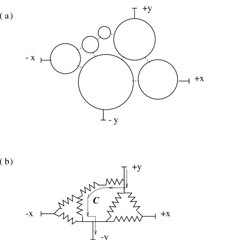
FIG. 2.: (a) A typical puddles–network (with $N_{v}=6$, $N_{b}=8$). (b) The corresponding equivalent circuit. The path ${\cal C}$ is denoted by arrows.

FIG. 3.: (a) An $S$–type element ($N_{s}=4$). (b) A $P$–type element ($N_{p}=4$).

REFERENCES

- [1] H. Fukuyama, J. Phys. Soc. Jpn. 49, 644 (1980); B. Altshuler, D. Khmelnitskii, A. Larkin and P. A. Lee, Phys. Rev. B 22, 5142 (1980).
- [2] S. C. Zhang, S. Kivelson and D. H. Lee, Phys. Rev. Lett. 69, 1252 (1992).
- [3] Y. Imry, Phys. Rev. Lett. 71, 1868 (1993).
- [4] O. Entin-Wohlman, A. G. Aronov, Y. Levinson and Y. Imry, Phys. Rev. Lett. 75, 4094 (1995).
- [5] P. Hopkins et al., Phys. Rev. B 39, 12708 (1989).
- [6] V. J. Goldman, M. Shayegan and D. C. Tsui, Phys. Rev. Lett. 61, 881 (1988); V. J. Goldman, J. K. Wang, B. Su and M. Shayegan, Phys. Rev. Lett. 70, 647 (1993); R. L. Willett, H. L. Stormer, D. C. Tsui, L. N. Pfeiffer, K. W. West and K. W. Baldwin, Phys. Rev. B 38, 7881 (1988).
- [7] D. Shahar, D. C. Tsui, M. Shayegan, E. Shimshoni and S. L. Sondhi, preprint (1995).
- [8] S. Kivelson, D. H. Lee and S. C. Zhang, Phys. Rev. B 46, 2223 (1992).
- [9] J. T. Chalker and P. D. Coddington, J. Phys. C 21, 2665 (1988).
- [10] Quantization of has been demonstrated for the critical regime: see A. M. Dykhne and I. M. Ruzin, Phys. Rev. B 50, 2369 (1994); I. M. Ruzin and S. Feng, Phys. Rev. Lett. 74, 154 (1995).
- [11] S.R. Renn and D.P. Arovas, Phys. Rev. B51, 16832 (1995).
- [12] C.W.J. Beenakker and H. van Hoiuten, Solid State Physics: Advances in Research and Applications, Ed. H. Ehrenreich and D. Turnbull ( Academic, San Diego, 1991), Vol 44, pp.207, 208.
- [13] This relation is more commonly known as , where are the vertices, faces, edges and Euler characteristics of general polygons in three dimensions.
- [14] X.-G. Wen, Int. Journ. Mod. Physics B, 6, 1711 (1992).
- [15] C. L. Kane and M. P. A. Fisher, Phys. Rev. B 46, 15233 (1992).
- [16] T. Giamarchi and H.J. Schultz, Phys. Rev. B37, 325 (1988).