Theory of Photoluminescence of the $\nu=1$ Quantum Hall State:
Excitons, Spin-Waves and Spin-Textures

Abstract

We study the theory of intrinsic photoluminescence of two-dimensional electron systems in the vicinity of the $\nu=1$ quantum Hall state. We focus predominantly on the recombination of a band of initial “excitonic states” that are the low-lying energy states of our model at $\nu=1$. It is shown that the recombination of excitonic states can account for recent observations of the polarization-resolved spectra of a high-mobility GaAs quantum well. The asymmetric broadening of the spectral line in the $\sigma_{-}$ polarization is explained to be the result of the “shake-up” of spin-waves upon radiative recombination of excitonic states. We derive line shapes for the recombination of excitonic states in the presence of long-range disorder that compare favourably with the experimental observations. We also discuss the stabilities and recombination spectra of other (“charged”) initial states of our model. An additional high-energy line observed in experiment is shown to be consistent with the recombination of a positively-charged state. The recombination spectrum of a negatively-charged initial state, predicted by our model but not observed in the present experiments, is shown to provide a direct measure of the formation energy of the smallest “charged spin-texture” of the $\nu=1$ state.

PACS numbers: 73.20.Dx, 71.35.-y, 75.30.Ds

I Introduction

Continuing improvements in the quality of quantum-well devices are leading to increasing resolution of the intrinsic photoluminescence spectra of two-dimensional electron systems in the extreme quantum regime. It is now well-established that features in the photoluminescence spectra are related to the appearance of the integer and fractional quantum Hall states and the insulating phase associated with the magnetically-induced Wigner crystal[1, 2, 3, 4]. The possibility of extracting information on the properties of these strongly-correlated phases from the photoluminescence spectra has stimulated a great deal of recent experimental and theoretical interest in this technique.

The interpretation of photoluminescence spectra requires an understanding of the energy eigenstates of a valence-band hole in the presence of the electron gas. Due to the strong many-body interactions that are important in the extreme quantum regime of these systems, this presents an essentially strongly-coupled many-body problem and the interpretation of spectral structure is extremely difficult. The theories that have been developed to address this issue fall into two broad categories. Certain theories treat the inter-particle correlations approximately through the use of some form of mean-field description of the interactions[5, 6, 7]. Such an approach has been shown to successfully account for oscillations in the mean position of the luminescence line in the integer quantum Hall regime of disordered samples[5]. The fractional quantum Hall and Wigner crystal regimes cannot be described within such a mean-field approach. To treat these cases, other theories have been developed which attempt to treat the inter-particle correlations more accurately[8, 9, 10, 11, 12, 13, 14, 15, 16]. In these theories, a simplified model is usually adopted in which the electrons and photo-excited hole are restricted to states in the lowest Landau level. For the most part, the resulting many-body problem has been treated by numerical diagonalization of small systems[8, 9, 10, 11, 12, 13], though some approximate analytic treatments have been proposed in the fractional quantum Hall[14, 15] and Wigner crystal[16] regimes. Despite the great deal of theoretical effort, the comparison between the theoretical and experimental photoluminescence spectra of high-mobility samples is still rather unsatisfactory, with even qualitative features of the observed spectra still not convincingly accounted for. (We note that “acceptor-bound photoluminescence” spectra are somewhat better understood[17, 18]. This experimental technique is quite different from intrinsic photoluminescence which we study here.)

It is the purpose of this paper to show that the intrinsic photoluminescence spectra of two-dimensional systems close to the integer filling fraction $\nu=1$ contain interesting and non-trivial structure (the filling fraction is defined by $\nu\equiv nh/eB$, where $n$ is the electron density and $eB/h$ the density of flux quanta). From a theoretical point of view, this is a much simpler filling fraction to study than the fractional quantum Hall and Wigner crystal regimes, yet still poses a non-trivial problem due to the importance of strong correlations in determining the low-energy excitations at this filling fraction.

In recent photoluminescence experiments on a very high-mobility GaAs quantum well, extremely narrow line widths have been achieved and very interesting low-energy structure has been resolved[19]. It is found that as the filling fraction of the sample is swept through $\nu=1$, the photoluminescence spectrum displays very intriguing behaviour. The evolution of the spectrum is quite different in the two circular polarizations, which originate from the recombination of a hole with electrons of the two spin-polarizations, as illustrated in Fig. 1(a). In one polarization ($\sigma_{+}$), no significant features are observed in the spectrum at $\nu=1$; the integrated intensity shows a weak minimum, but the line shape is almost unchanged. In the other polarization ($\sigma_{-}$), a much more dramatic evolution is observed: the integrated intensity also decreases slightly, but, at the same time, the main spectral line becomes strongly broadened on the low-energy side; at the lowest temperatures, an additional high-energy peak appears. Figure 1(b) shows the spectra observed in the experiments reported in Ref. [19] at the filling fraction $\nu=1$ for both circular polarizations; the additional high-energy peak is labelled the “B-peak”.

FIG. 1.: (a) Schematic diagram of the low-energy interband transitions in a GaAs quantum well. The recombination of electrons of the two spin orientations of the lowest Landau level gives rise to the two different circular polarizations. (b) Low-temperature photoluminescence spectra of a GaAs quantum well at $\nu=1$, from the experiments reported in Ref. [19]. In the $\sigma_{+}$ circular polarization, a narrow line is observed with a line shape similar to that observed away from $\nu=1$. In the $\sigma_{-}$ circular polarization, the spectrum acquires a strong low-energy broadening as compared to the spectra away from $\nu=1$; an additional high-energy peak (peak B) appears at low temperatures. Energies are measured relative to the energies at which the intensities are maximal.

These observations cannot be accounted for within the existing “mean-field” theories of photoluminescence in the integer quantum Hall regime[5, 6, 7]. In the first place, these theories treat the spin-degree of freedom of the electrons in such a way that no polarization-dependent effects can appear. Moreover, strong correlations are likely to be important in determining the structure observed in photoluminescence at $\nu=1$, since it is now clear that the properties of typical GaAs systems at this filling fraction are dominated by interactions, the single particle gap (the bare electron Zeeman energy) being very much smaller than the interaction energy scale. In fact, as suggested in Ref.[20], the $\nu=1$ state is better viewed as a strongly-correlated state similar to the incompressible states at fractional filling fraction, since, even for a vanishing single-particle gap, a quantized Hall effect would appear at $\nu=1$ as a result of the electron-electron repulsion. This state has received a great deal of recent theoretical[20, 21, 22] and experimental interest[23, 24, 25], in an effort to understand the effects of the electron spin on the properties of the low-energy excitations. In this light, it is of particular interest to understand the origin of the structure appearing in the above photoluminescence spectra, since this technique separately probes the two spin states of the electrons.

Motivated by these experiments, we study the theory of the intrinsic photoluminescence of two-dimensional electron systems at filling fractions close to $\nu=1$. We will follow the models used in the fractional quantum Hall and Wigner crystal regimes and neglect Landau level mixing for the electrons, but will take full account of the inter-particle correlations. The model that one obtains within this approximation is much simpler to analyse at $\nu=1$ than in either of these other two regimes. Therefore, at the very least, the study of this model at $\nu=1$ is the most natural way in which to test the applicability of the underlying assumptions of the theories for photoluminescence in the fractional quantum Hall and Wigner crystal regimes. Moreover, as we shall see, the photoluminescence spectrum at $\nu=1$ retains non-trivial structure related to the low-energy excitations of this state and is therefore of great interest in itself. A similar approach to photoluminescence at $\nu=1$ has been discussed in Ref.[26]. This work did not address the polarization-dependence of the photoluminescence spectrum. We study these issues in some detail, and compare our predictions with the experimental observations described above. We show that one can account for all of the qualitative features observed in the experiment.

The outline of the paper is as follows. In Sec. II we motivate the model that we will study, and discuss its relationship with other models of photoluminescence in the extreme quantum regime. In Sec. III, we study the predictions of this model at a filling fraction of exactly $\nu=1$. We argue that for the sample studied in Ref. [19], and for all samples in which the valence-band hole is close to the electron gas compared to the typical electron-electron spacing, the most important initial states are “excitonic states” (as we choose to name them). These are states in which the Landau level of spin-$\uparrow$ electrons is fully occupied, and the valence-band hole binds with a spin-$\downarrow$ electron to form an exciton. In the remainder of this section we study the photoluminescence spectrum arising from the recombination of these excitonic states. This is the main part of the paper, and contains our most important conclusions with regard to the experimental observations. The radiative recombination of the excitonic states is shown to be quite different in the two circular polarizations. In the $\sigma_{+}$ polarization, the hole recombines with the spin-$\downarrow$ electron to which it is bound, leaving an undisturbed Landau level of spin-$\uparrow$ electrons. In the $\sigma_{-}$ polarization, the hole recombines with one of the spin-$\uparrow$ electrons, and a single spin-reversal is left in the final state. The photoluminescence spectrum in this polarization becomes broadened to low energy due to the “shake-up” of these spin-waves. We argue that the polarization-dependence of the main recombination line in the spectra of Fig. 1(b) can be accounted for in terms of the recombination of excitonic states: the recombination line in the $\sigma_{-}$ polarization is broadened to low energy due to the shake-up of spin-waves, while the line in the $\sigma_{+}$ polarization remains narrow (with a width limited only by disorder). We derive the line shapes for a disorder-free system as a function of the separation between valence-band hole and electron gas and the extent of Landau level mixing for the hole. We show that disorder arising from the remote ionized donor impurities is likely to have an important effect on the width of this line, and derive line shapes for the recombination in the two polarizations taking account of this disorder. The line shapes compare favourably with the experimental observations shown in Fig. 1(b).

In Sec. IV, we turn our attention to quite different initial states, in which the valence-band hole forms a positively-charged or negatively-charged complex. These states can have lower energies than the excitonic states if the filling fraction is slightly less than or greater than $\nu=1$ (when some quasiparticles are present), and can then be important for photoluminescence. We show that the high-energy line (peak B) in Fig. 1(b) is consistent with the recombination of a positively-charged initial state in which there are no spin-$\downarrow$ electrons in the vicinity of the hole. In this case, our calculations include corrections arising from Landau level mixing for the electrons. These are shown to change the position of this recombination line relative to that of the excitonic states. The recombination spectrum of a negatively-charged initial state is shown, from numerical studies, to contain structure that measures the formation energy of the smallest “charged spin-texture”[20, 21, 22] of the $\nu=1$ state. There is no clear evidence for this initial state in the present experiments. We discuss the type of sample and the conditions under which this initial state might be more stable and its recombination could be observed. Finally, Sec. V contains a summary of the main points of the paper.

II Description of the model

We aim to develop a theory that can account for the photoluminescence of high-mobility quantum wells in the vicinity of $\nu=1$. In the experiments of Ref. [19], and in experiments on similar GaAs quantum wells[4], recombination is observed between the two lowest-energy electron states (the two spin-polarizations of the lowest Landau level of the lowest subband state), and the two lowest-energy hole states. These two hole states originate from the heavy-hole states of the valence band, but are strongly mixed with the light-hole states due to the quantum well confinement[27]. Typically, sufficiently low excitation powers are used that the density of holes is extremely small (compared to the density of electrons) and they may be considered to be independent.

To represent these systems, we will study a model in which the electrons are confined to a single subband and carry a spin of $1/2$, and there is a single hole, which may be in one of the two states ($\Uparrow$ or $\Downarrow$)[28]. Since we consider the recombination of a single photo-excited hole, the “spin” label of the hole will play no role other than to define the polarization in which the hole can recombine [see Fig. 1(a)]. We will therefore ignore this label, and leave it to be understood that when we discuss a recombination process with a spin-$\uparrow$ (spin-$\downarrow$) electron the hole must be in the spin-$\Uparrow$ (spin-$\Downarrow$) state.

For the most part, we will assume that following photo-excitation the system is able to relax to thermal equilibrium before the hole recombines. In this case, one can understand the photoluminescence spectrum by identifying the low-lying energy eigenstates of a single photo-excited hole in the presence of the electron gas, and studying the processes by which these states can decay radiatively. The rate of each interband transition is determined by the matrix element of the electric dipole operator between the initial and final states. Within the effective mass approximation, this is proportional to the matrix element of one of the operators

$$L_{-} \equiv \int d^{2}\mathchoice{{\hbox{\boldmath$\displaystyle r$}}}{{\hbox{\boldmath$\textstyle r$}}}{{\hbox{\boldmath$\scriptstyle r$}}}{{\hbox{\boldmath$\scriptscriptstyle r$}}}\;\psi_{e\uparrow}(\mathchoice{{\hbox{\boldmath$\displaystyle r$}}}{{\hbox{\boldmath$\textstyle r$}}}{{\hbox{\boldmath$\scriptstyle r$}}}{{\hbox{\boldmath$\scriptscriptstyle r$}}})\psi_{h\Uparrow}(\mathchoice{{\hbox{\boldmath$\displaystyle r$}}}{{\hbox{\boldmath$\textstyle r$}}}{{\hbox{\boldmath$\scriptstyle r$}}}{{\hbox{\boldmath$\scriptscriptstyle r$}}}),$$ (1)

$$L_{+} \equiv \int d^{2}\mathchoice{{\hbox{\boldmath$\displaystyle r$}}}{{\hbox{\boldmath$\textstyle r$}}}{{\hbox{\boldmath$\scriptstyle r$}}}{{\hbox{\boldmath$\scriptscriptstyle r$}}}\;\psi_{e\downarrow}(\mathchoice{{\hbox{\boldmath$\displaystyle r$}}}{{\hbox{\boldmath$\textstyle r$}}}{{\hbox{\boldmath$\scriptstyle r$}}}{{\hbox{\boldmath$\scriptscriptstyle r$}}})\psi_{h\Downarrow}(\mathchoice{{\hbox{\boldmath$\displaystyle r$}}}{{\hbox{\boldmath$\textstyle r$}}}{{\hbox{\boldmath$\scriptstyle r$}}}{{\hbox{\boldmath$\scriptscriptstyle r$}}}),$$ (2)

between the in-plane envelope functions of the initial and final states, $\psi_{(e,h)\sigma}(\mathchoice{{\hbox{\boldmath$\displaystyle r$}}}{{\hbox{\boldmath$\textstyle r$}}}{{\hbox{\boldmath$\scriptstyle r$}}}{{\hbox{\boldmath$\scriptscriptstyle r$}}})$ being the electron and hole field annihilation operators. The absolute transition rate depends on the overlap of the electron and hole subband wavefunctions, and on the form of the electron and hole wavefunctions on an atomic scale, which may differ for the two polarizations. We will study only the contributions arising from the matrix elements of $L_{\pm}$, which are sufficient to determine the line shapes in the two polarizations.

Due to the importance of many-body interactions in the quantized Hall regime of these systems, to make progress one must restrict attention to a somewhat simplified model of the initial and final states of the photoluminescence process. A natural model to study which retains the effects of many-body correlations is one in which the electrons and the hole are restricted to the lowest Landau level and move in a single plane. Such a model is motivated by the success of similar approximations in accounting for the qualitative and quantitative properties of the $\nu=1$ state and the incompressible states at fractional filling fractions[29]. However, various authors[30, 31, 32, 13, 9] have shown that for spin-polarized electrons and holes restricted to a single Landau level and with the same quantum well envelope functions, a “hidden symmetry” leads to the result that photoluminescence contains no spectroscopic structure: the spectrum consists of a single line at an energy that is independent of the state, or even the presence, of the electron gas. In the present case, the electrons are not spin-polarized. However, it is straightforward to show that a similar symmetry applies for an arbitrary number of spin components for electrons and holes, provided the interactions conserve the spin of each particle: the spectrum consists of a series of sharp lines, at energies which are independent of the state or presence of the electron gas (these are therefore the energies of each allowed interband transition for an empty quantum well).

In order to obtain a non-trivial photoluminescence spectrum, it is essential to study a model that breaks this symmetry. There are two clear mechanisms by which this occurs in practice. Firstly, through Landau level coupling for the electrons or hole; in GaAs quantum wells, this is likely to be more important for the hole than for the electrons due to the much smaller cyclotron energy of the valence band compared to that of the conduction band. Secondly, due to the asymmetry of the single-side-doped quantum wells and single heterojunctions used in the experiments, the electrons and holes do not move in the same plane; the hole is pulled somewhat away from the electron layer[33]. Note that the presence of a disordered potential does not break the symmetry, and one of the above two mechanisms must be introduced.

It is common in theories of photoluminescence in the fractional quantum Hall regime to retain Landau quantization for both electrons and holes and to break the “hidden symmetry” by introducing a separation $d$ between the planes in which the electrons and hole move[9, 11]. In our work, we will restrict the electrons to states in the lowest Landau level, and will also assume that the electrons and the hole are confined to planes that are separated by a distance $d$. We will not, however, impose the restriction that the hole is in the lowest Landau level. We take account of Landau level mixing for the valence-band hole by assuming its in-plane dispersion to be parabolic with an effective mass $m_{h}$. Thus we retain two mechanisms by which the hidden symmetry is broken. We will discuss how the photoluminescence spectrum depends on the parameters, $d$ and $m_{h}$. For quantitative comparisons of our theory with the experimental observations reproduced in Fig. 1(b), we will choose $d$ to be the separation between the centres of the electron and hole subband wavefunctions in the quantum well used in these experiments, which is approximately $60\mbox{\AA}$[34] and is therefore small compared to the magnetic length $\ell=130\mbox{\AA}$ under these conditions (the magnetic length, $\ell\equiv\sqrt{\hbar/eB}$, is a measure of the size of a single-particle state in the lowest Landau level and is therefore a fundamental lengthscale in our model). In the absence of detailed knowledge of the valence band dispersion, which depends strongly on the shape of the quantum well[35], we will choose the value $m_{h}=0.34m_{0}$ for both hole states; this is typical of the masses measured in experiment[35] and is the value used in theoretical studies of related problems[36]. Thus, under these conditions the ratio of the cyclotron energy of the hole, $\hbar\omega_{h}\equiv\hbar eB/m_{h}$, to the typical interaction energy scale, $e^{2}/4\pi\epsilon\epsilon_{0}\ell$, is rather small, 0.15 (using $\epsilon=12.53$ for GaAs), and one can expect Landau level mixing for the hole to be quantitatively important. Indeed, we will show that it is the finite mass of the hole that provides the more important mechanism by which the “hidden symmetry” is broken in the photoluminescence spectrum.

The neglect of Landau level mixing for the electrons is the principal assumption of our work and leads to the key simplifications. It allows explicit knowledge of the groundstate of the system at $\nu=1$: a filled Landau level of spin-$\uparrow$ electrons[20]. Moreover, we shall always consider interactions which preserve the electron spin. Therefore, prior to recombination of the valence-band hole, the system may be characterized by the number of spin-$\downarrow$ electrons and the number of missing spin-$\uparrow$ electrons in the otherwise filled lowest Landau level (“spin-holes”). Through the use of this particle-hole transformation, the initial states may described by the interaction of the hole with (spin-$\downarrow$) electrons and spin-holes, both restricted to states in the lowest Landau level. For filling fractions close to $\nu=1$, and for states which do not involve a large degree of spin-depolarization, relatively few of these particles are present, and the calculation of the energy eigenstates poses a few-body problem. The majority of our work will address the properties of the system in which there are only two such particles; our results in this case are based on analytical treatments. We will also present results of numerical studies for systems with larger numbers of particles. We work in the spherical geometry[37, 38] and introduce the separation $d$ between the electrons and hole in the same way as was done in Ref. [8]. For all of the calculations that we report, the system size is sufficiently large that finite-size effects are well-controlled.

Although the neglect of Landau level mixing is not likely to be quantitatively accurate at weak fields, when the typical interaction energy can be larger than the electron cyclotron energy, we hope that it does give the correct qualitative picture. In Sec. III F, we will indicate the extent to which one can trust the qualitative features of a model neglecting Landau level mixing for the electrons, and in Sec. IV A will calculate some quantitative corrections arising from this mixing.

III Excitonic States

In this section we will consider the introduction of an electron-hole pair to the groundstate at $\nu=1$. We will show that, provided that the distance $d$ of the hole from the electron gas is not too large, the low-energy states may be described by a band of “excitonic states”, defined below. We will further show that the recombination of these excitonic states can account for the main feature of the spectra presented in Fig. 1(b): a sharp recombination line in the $\sigma_{+}$ polarization and an asymmetrically broadened line in $\sigma_{-}$. We will develop models for the line shapes in the two polarizations; first for a system with no disorder, and then taking account of the long-range disorder arising from remote ionized donors. We will compare the predictions of these models with the experimental observations.

A Definition of the Excitonic States

As we have explained above, the principal assumption throughout our discussion is that the electrons are confined to the lowest Landau level. In this case, the groundstate of the system at $\nu=1$ prior to photo-excitation is the state

$$|0\rangle\equiv\prod_{m}e_{m\uparrow}^{\dagger}|\mbox{vac}\rangle,$$ (3)

in which the electrons fill all the spin-$\uparrow$ states in the lowest Landau level and all spin-$\downarrow$ states are unoccupied. In the above expression, $|\mbox{vac}\rangle$ is the vacuum state with a filled valence band and empty conduction band, and $e_{m\sigma}^{\dagger}$ is the operator which creates a spin-$\sigma$ electron in a single particle state in the lowest Landau level. The quantum number $m$ is any internal quantum number that runs over all degenerate states in the lowest Landau level. This state is clearly the absolute groundstate if the bare electron Zeeman energy, $Z$, is large compared to the typical interaction energy, set by $e^{2}/4\pi\epsilon\epsilon_{0}\ell$. Due to the spontaneous ferromagnetism which appears for repulsive electron-electron interactions, it is also the groundstate in the limit $Z\rightarrow 0$[20].

We now consider the introduction of an additional electron-hole pair to the system. The properties of the low-energy states depend on all of the model parameters: $d/\ell$ and the ratios of the cyclotron energy of the hole, $\hbar\omega_{h}$, and the electron Zeeman energy, $Z$, to the typical interaction energy scale $e^{2}/4\pi\epsilon\epsilon_{0}\ell$. However, if the Zeeman energy is large compared to the interaction energy, the low-energy states will be maximally spin-polarized, and their form is clear: all of the spin-$\uparrow$ electron states will be occupied, and there will be one remaining spin-$\downarrow$ electron which will bind with the valence-band hole to form an exciton (in a magnetic field, any attractive interaction will lead to binding of a two-dimensional electron-hole pair). We refer to these states as “excitonic states”. Since we assume that all interactions conserve the electron spin and we ignore Landau level mixing for the electrons, the filled Landau level of spin-$\uparrow$ electrons is inert, and the properties of the excitonic states may be determined by considering only the electron-hole pair. In particular, the energy eigenstates of the system follow from those of the exciton itself. The state in which the exciton is in a state $\Psi_{P}(\mathchoice{{\hbox{\boldmath$\displaystyle r$}}}{{\hbox{\boldmath$\textstyle r$}}}{{\hbox{\boldmath$\scriptstyle r$}}}{{\hbox{\boldmath$\scriptscriptstyle r$}}}_{e},\mathchoice{{\hbox{\boldmath$\displaystyle r$}}}{{\hbox{\boldmath$\textstyle r$}}}{{\hbox{\boldmath$\scriptstyle r$}}}{{\hbox{\boldmath$\scriptscriptstyle r$}}}_{h})$ with momentum $\textstyle P$ is

$$|\mathchoice{{\hbox{\boldmath$\displaystyle P$}}}{{\hbox{\boldmath$\textstyle P$}}}{{\hbox{\boldmath$\scriptstyle P$}}}{{\hbox{\boldmath$\scriptscriptstyle P$}}}\rangle\equiv\int d^{2}\mathchoice{{\hbox{\boldmath$\displaystyle r$}}}{{\hbox{\boldmath$\textstyle r$}}}{{\hbox{\boldmath$\scriptstyle r$}}}{{\hbox{\boldmath$\scriptscriptstyle r$}}}_{e}d^{2}\mathchoice{{\hbox{\boldmath$\displaystyle r$}}}{{\hbox{\boldmath$\textstyle r$}}}{{\hbox{\boldmath$\scriptstyle r$}}}{{\hbox{\boldmath$\scriptscriptstyle r$}}}_{h}\;\Psi_{P}(\mathchoice{{\hbox{\boldmath$\displaystyle r$}}}{{\hbox{\boldmath$\textstyle r$}}}{{\hbox{\boldmath$\scriptstyle r$}}}{{\hbox{\boldmath$\scriptscriptstyle r$}}}_{e},\mathchoice{{\hbox{\boldmath$\displaystyle r$}}}{{\hbox{\boldmath$\textstyle r$}}}{{\hbox{\boldmath$\scriptstyle r$}}}{{\hbox{\boldmath$\scriptscriptstyle r$}}}_{h})\psi_{e\downarrow}^{\dagger}(\mathchoice{{\hbox{\boldmath$\displaystyle r$}}}{{\hbox{\boldmath$\textstyle r$}}}{{\hbox{\boldmath$\scriptstyle r$}}}{{\hbox{\boldmath$\scriptscriptstyle r$}}}_{e})\psi_{h}^{\dagger}(\mathchoice{{\hbox{\boldmath$\displaystyle r$}}}{{\hbox{\boldmath$\textstyle r$}}}{{\hbox{\boldmath$\scriptstyle r$}}}{{\hbox{\boldmath$\scriptscriptstyle r$}}}_{h})|0\rangle.$$ (4)

We have suppressed the subband-label of the hole, but it is to be understood that there are two excitonic bands corresponding to the two hole states. In the absence of an external potential, the momentum $\textstyle P$ is conserved and the above states are energy eigenstates. In appendix A the wavefunctions and dispersion relation of a two-dimensional exciton are derived at small momentum as a function of $m_{h}$ and $d$, within the approximation of no Landau level mixing for the electron.

B Stability to Spin Reversal

The above excitonic states are the low-energy eigenstates of the system when the Zeeman energy is large compared to the interaction energy scale. However, for typical GaAs samples at $\nu=1$, the Zeeman energy of electrons is much smaller than the interaction energy scale (at 4T the Zeeman energy is 0.09meV, whereas the typical interaction energy is $e^{2}/4\pi\epsilon\epsilon_{0}\ell=8.9\mbox{meV}$). It is therefore important, for practical purposes, to study whether these excitonic states remain the lowest-energy states when the Zeeman energy is small. It is possible that there exist lower energy states involving some degree of spin depolarization. Such depolarization is known to be important for the charged excitations of this system, for which theoretical[20, 21, 22] and some experimental[23, 24, 25] studies show that the lowest energy charged excitations are “charged spin-textures” which diverge in size to become “skyrmions” in the limit of vanishing Zeeman energy.

The spin-polarization of the groundstate depends strongly on the system parameters ($d$, $m_{h}$ and $Z$). For sufficiently large $d$, the system will become depolarized when $Z$ is small: in this case, the interactions between the electron gas and the hole may be neglected and the groundstate spin polarization will be that of the extra electron, which is determined by the lowest-energy charged spin-texture. However, for small $d$ the hole is tightly bound to the additional electron, and it is possible that the resulting neutral exciton does not significantly disturb the spin-polarization of the remaining electrons.

We have studied the stability of the exciton state to spin-reversal by calculating the groundstate of the system in the presence of a single spin-reversal. Our calculations were performed in the spherical geometry, with system sizes of up to 51 single particle basis states in the lowest Landau level (corresponding to a sphere of diameter $10\ell$). We have studied only the limiting cases $m_{h}=0,\infty$ and assume that the results for finite hole mass lie between these two limits. We find that, for $m_{h}=0$ and $m_{h}=\infty$, the groundstate is the global spin-rotation of the excitonic groundstate provided $d<1.4\ell$ and $d<1.3\ell$, respectively (we have identified these values to an accuracy of better than $\pm 0.1\ell$). Therefore, for $d$ smaller than these values, there is no energetic advantage to be gained from introducing a single spin-flip to the excitonic state: the zero-momentum excitonic state remains the groundstate. In order to fully test the stability of the excitonic state to spin-reversal, one should study the groundstate as a function of all possible spin-polarizations. However, it seems likely that if the energy is not reduced by the introduction of a single spin-reversal, it will not be reduced by a larger depolarization. We therefore anticipate that for $d$ smaller than $1.3\ell$, the $\mathchoice{{\hbox{\boldmath$\displaystyle P$}}}{{\hbox{\boldmath$\textstyle P$}}}{{\hbox{\boldmath$\scriptstyle P$}}}{{\hbox{\boldmath$\scriptscriptstyle P$}}}=0$ excitonic state is the absolute groundstate of our model whatever value the hole mass may take, and even as $Z\rightarrow 0$. For larger values of $d$, the spin-polarization of the groundstate will change as $Z$ is decreased; one may view the resulting depolarized states as excitons formed from the binding of a valence-band hole with a charged spin-texture.

For the parameter-values that we use to compare with the experiments reported in Ref. [19] the spacing $d=60\mbox{\AA}$ is much less than the magnetic length $\ell=130\mbox{\AA}$. Our calculations therefore suggest that in this sample the hole is sufficiently close to the electron gas that the $\mathchoice{{\hbox{\boldmath$\displaystyle P$}}}{{\hbox{\boldmath$\textstyle P$}}}{{\hbox{\boldmath$\scriptstyle P$}}}{{\hbox{\boldmath$\scriptscriptstyle P$}}}=0$ excitonic state provides a good description of the groundstate of the system exactly at $\nu=1$ prior to recombination. We therefore expect the excitonic states to provide an important contribution to the photoluminescence spectrum of this sample.

At finite temperatures, some of the low-energy excited states of the system will also be populated. These will consist both of finite-momentum exciton states, and of long-wavelength spin-wave excitations of the system. For small electron-hole separation, $d$, and for sufficiently small excitation energies that the wavelengths of these excitations are large compared to the magnetic length, the coupling between the exciton and spin-waves will be small, and the two may be treated independently. In the remainder of this section we will discuss the form of recombination expected from the excitonic states in the absence of spin-waves. A thermal population of spin-waves may be viewed as a fluctuation in the overall polarization of the system, and will lead to a mixing between the two circular polarizations of the spectra. Provided the temperature is small compared to the particle-hole gap at $\nu=1$, only a small number of spin-waves will be thermally populated, and this mixing will be small.

C Radiative Recombination

It is clear from the form of the excitonic states described above that their radiative recombination in the two circular polarizations will lead to quite different final states. In the $\sigma_{+}$ polarization, the hole (which must be in the $\Downarrow$ state) must recombine with the single spin-$\downarrow$ electron. In this case, there is only one available final state: the $\nu=1$ groundstate (3). In the $\sigma_{-}$ polarization, the hole can recombine with any one of the spin-$\uparrow$ electrons and there are many possible final states. These are the states in which the spin of a single electron has been reversed in the $\nu=1$ groundstate, and are described by the set of single spin-wave excitations[39, 40]. The recombination processes in the two polarizations are illustrated schematically in Fig. 2.

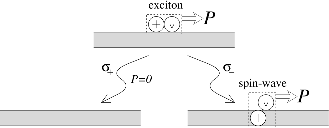
FIG. 2.: Schematic diagram of the radiative decay processes of the free excitonic states. Each shaded region represents a filled Landau level of spin-$\uparrow$ electrons, and the circles represent a spin-$\downarrow$ electron (marked by $\downarrow$), a valence-band hole (lying above the shaded region and marked by $+$), and a “spin-hole” (lying in the shaded region and marked by $+$).

The transition rates of these processes are determined by the matrix elements of the operators, $L_{\pm}$. Using the form of the exciton wavefunctions derived in appendix A, these matrix elements can be calculated explicitly.

We find that the matrix element describing $\sigma_{+}$ recombination between the excitonic state $|\mathchoice{{\hbox{\boldmath$\displaystyle P$}}}{{\hbox{\boldmath$\textstyle P$}}}{{\hbox{\boldmath$\scriptstyle P$}}}{{\hbox{\boldmath$\scriptscriptstyle P$}}}\rangle$ and the groundstate $|0\rangle$ is

$$\langle 0|L_{+}|\mathchoice{{\hbox{\boldmath$\displaystyle P$}}}{{\hbox{\boldmath$\textstyle P$}}}{{\hbox{\boldmath$\scriptstyle P$}}}{{\hbox{\boldmath$\scriptscriptstyle P$}}}\rangle=\sqrt{\frac{\Omega}{2\pi\ell^{2}}}\;\delta_{P,0},$$ (5)

where $\Omega$ is the area of the sample. Thus, on emission of a long-wavelength photon, momentum conservation limits the recombination to the zero-momentum excitonic state.

As we now show, for the $\sigma_{-}$ polarization all of the excitonic states can recombine, with the momentum of the exciton being conserved by the momentum of the spin-wave in the final state. Making a particle-hole transformation on the filled Landau level of spin-$\uparrow$ electrons, the matrix element of $L_{-}$ between an initial excitonic state, $|\mathchoice{{\hbox{\boldmath$\displaystyle P$}}}{{\hbox{\boldmath$\textstyle P$}}}{{\hbox{\boldmath$\scriptstyle P$}}}{{\hbox{\boldmath$\scriptscriptstyle P$}}}\rangle$, and a final state $|\mathchoice{{\hbox{\boldmath$\displaystyle P$}}}{{\hbox{\boldmath$\textstyle P$}}}{{\hbox{\boldmath$\scriptstyle P$}}}{{\hbox{\boldmath$\scriptscriptstyle P$}}}^{\prime}\rangle_{SW}$ in which there is a single spin-wave with momentum $\mathchoice{{\hbox{\boldmath$\displaystyle P$}}}{{\hbox{\boldmath$\textstyle P$}}}{{\hbox{\boldmath$\scriptstyle P$}}}{{\hbox{\boldmath$\scriptscriptstyle P$}}}^{\prime}$, may be written

$$_{SW}\langle\mathchoice{{\hbox{\boldmath$\displaystyle P$}}}{{\hbox{\boldmath$\textstyle P$}}}{{\hbox{\boldmath$\scriptstyle P$}}}{{\hbox{\boldmath$\scriptscriptstyle P$}}}^{\prime}|L_{-}|\mathchoice{{\hbox{\boldmath$\displaystyle P$}}}{{\hbox{\boldmath$\textstyle P$}}}{{\hbox{\boldmath$\scriptstyle P$}}}{{\hbox{\boldmath$\scriptscriptstyle P$}}}\rangle=\int\Psi_{SW,\mathchoice{{\hbox{\boldmath$\displaystyle P$}}}{{\hbox{\boldmath$\textstyle P$}}}{{\hbox{\boldmath$\scriptstyle P$}}}{{\hbox{\boldmath$\scriptscriptstyle P$}}}}^{*}(\mathchoice{{\hbox{\boldmath$\displaystyle r$}}}{{\hbox{\boldmath$\textstyle r$}}}{{\hbox{\boldmath$\scriptstyle r$}}}{{\hbox{\boldmath$\scriptscriptstyle r$}}}_{e},\mathchoice{{\hbox{\boldmath$\displaystyle r$}}}{{\hbox{\boldmath$\textstyle r$}}}{{\hbox{\boldmath$\scriptstyle r$}}}{{\hbox{\boldmath$\scriptscriptstyle r$}}}_{h})\Psi_{X,\mathchoice{{\hbox{\boldmath$\displaystyle P$}}}{{\hbox{\boldmath$\textstyle P$}}}{{\hbox{\boldmath$\scriptstyle P$}}}{{\hbox{\boldmath$\scriptscriptstyle P$}}}}(\mathchoice{{\hbox{\boldmath$\displaystyle r$}}}{{\hbox{\boldmath$\textstyle r$}}}{{\hbox{\boldmath$\scriptstyle r$}}}{{\hbox{\boldmath$\scriptscriptstyle r$}}}_{e},\mathchoice{{\hbox{\boldmath$\displaystyle r$}}}{{\hbox{\boldmath$\textstyle r$}}}{{\hbox{\boldmath$\scriptstyle r$}}}{{\hbox{\boldmath$\scriptscriptstyle r$}}}_{h})\;d^{2}\mathchoice{{\hbox{\boldmath$\displaystyle r$}}}{{\hbox{\boldmath$\textstyle r$}}}{{\hbox{\boldmath$\scriptstyle r$}}}{{\hbox{\boldmath$\scriptscriptstyle r$}}}_{e}d^{2}\mathchoice{{\hbox{\boldmath$\displaystyle r$}}}{{\hbox{\boldmath$\textstyle r$}}}{{\hbox{\boldmath$\scriptstyle r$}}}{{\hbox{\boldmath$\scriptscriptstyle r$}}}_{h},$$ (6)

where $\Psi_{X,P}(\mathchoice{{\hbox{\boldmath$\displaystyle r$}}}{{\hbox{\boldmath$\textstyle r$}}}{{\hbox{\boldmath$\scriptstyle r$}}}{{\hbox{\boldmath$\scriptscriptstyle r$}}}_{e},\mathchoice{{\hbox{\boldmath$\displaystyle r$}}}{{\hbox{\boldmath$\textstyle r$}}}{{\hbox{\boldmath$\scriptstyle r$}}}{{\hbox{\boldmath$\scriptscriptstyle r$}}}_{h})$ and $\Psi_{SW,P}(\mathchoice{{\hbox{\boldmath$\displaystyle r$}}}{{\hbox{\boldmath$\textstyle r$}}}{{\hbox{\boldmath$\scriptstyle r$}}}{{\hbox{\boldmath$\scriptscriptstyle r$}}}_{e},\mathchoice{{\hbox{\boldmath$\displaystyle r$}}}{{\hbox{\boldmath$\textstyle r$}}}{{\hbox{\boldmath$\scriptstyle r$}}}{{\hbox{\boldmath$\scriptscriptstyle r$}}}_{h})$ are the wavefunctions of the exciton and spin-wave of momentum $\textstyle P$, with $\mathchoice{{\hbox{\boldmath$\displaystyle r$}}}{{\hbox{\boldmath$\textstyle r$}}}{{\hbox{\boldmath$\scriptstyle r$}}}{{\hbox{\boldmath$\scriptscriptstyle r$}}}_{h}$ representing the position of the spin-hole in the second case. In the symmetric gauge, $\mathchoice{{\hbox{\boldmath$\displaystyle A$}}}{{\hbox{\boldmath$\textstyle A$}}}{{\hbox{\boldmath$\scriptstyle A$}}}{{\hbox{\boldmath$\scriptscriptstyle A$}}}(\mathchoice{{\hbox{\boldmath$\displaystyle r$}}}{{\hbox{\boldmath$\textstyle r$}}}{{\hbox{\boldmath$\scriptstyle r$}}}{{\hbox{\boldmath$\scriptscriptstyle r$}}})=B\hat{\mathchoice{{\hbox{\boldmath$\displaystyle z$}}}{{\hbox{\boldmath$\textstyle z$}}}{{\hbox{\boldmath$\scriptstyle z$}}}{{\hbox{\boldmath$\scriptscriptstyle z$}}}}\times\mathchoice{{\hbox{\boldmath$\displaystyle r$}}}{{\hbox{\boldmath$\textstyle r$}}}{{\hbox{\boldmath$\scriptstyle r$}}}{{\hbox{\boldmath$\scriptscriptstyle r$}}}/2$, the exciton and spin-wave wavefunctions may be written[41]

$$\Psi_{P}(\mathchoice{{\hbox{\boldmath$\displaystyle r$}}}{{\hbox{\boldmath$\textstyle r$}}}{{\hbox{\boldmath$\scriptstyle r$}}}{{\hbox{\boldmath$\scriptscriptstyle r$}}}_{e},\mathchoice{{\hbox{\boldmath$\displaystyle r$}}}{{\hbox{\boldmath$\textstyle r$}}}{{\hbox{\boldmath$\scriptstyle r$}}}{{\hbox{\boldmath$\scriptscriptstyle r$}}}_{h})=\frac{1}{\sqrt{\Omega}}e^{i\mathchoice{{\hbox{\boldmath$\displaystyle P$}}}{{\hbox{\boldmath$\textstyle P$}}}{{\hbox{\boldmath$\scriptstyle P$}}}{{\hbox{\boldmath$\scriptscriptstyle P$}}}.(\mathchoice{{\hbox{\boldmath$\displaystyle r$}}}{{\hbox{\boldmath$\textstyle r$}}}{{\hbox{\boldmath$\scriptstyle r$}}}{{\hbox{\boldmath$\scriptscriptstyle r$}}}_{e}+\mathchoice{{\hbox{\boldmath$\displaystyle r$}}}{{\hbox{\boldmath$\textstyle r$}}}{{\hbox{\boldmath$\scriptstyle r$}}}{{\hbox{\boldmath$\scriptscriptstyle r$}}}_{h})/2\hbar}e^{i\mathchoice{{\hbox{\boldmath$\displaystyle r$}}}{{\hbox{\boldmath$\textstyle r$}}}{{\hbox{\boldmath$\scriptstyle r$}}}{{\hbox{\boldmath$\scriptscriptstyle r$}}}_{e}\times\mathchoice{{\hbox{\boldmath$\displaystyle r$}}}{{\hbox{\boldmath$\textstyle r$}}}{{\hbox{\boldmath$\scriptstyle r$}}}{{\hbox{\boldmath$\scriptscriptstyle r$}}}_{h}.\hat{\mathchoice{{\hbox{\boldmath$\displaystyle z$}}}{{\hbox{\boldmath$\textstyle z$}}}{{\hbox{\boldmath$\scriptstyle z$}}}{{\hbox{\boldmath$\scriptscriptstyle z$}}}}/2\ell^{2}}\Phi_{\mathchoice{{\hbox{\boldmath$\displaystyle P$}}}{{\hbox{\boldmath$\textstyle P$}}}{{\hbox{\boldmath$\scriptstyle P$}}}{{\hbox{\boldmath$\scriptscriptstyle P$}}}}(\mathchoice{{\hbox{\boldmath$\displaystyle r$}}}{{\hbox{\boldmath$\textstyle r$}}}{{\hbox{\boldmath$\scriptstyle r$}}}{{\hbox{\boldmath$\scriptscriptstyle r$}}}_{e}-\mathchoice{{\hbox{\boldmath$\displaystyle r$}}}{{\hbox{\boldmath$\textstyle r$}}}{{\hbox{\boldmath$\scriptstyle r$}}}{{\hbox{\boldmath$\scriptscriptstyle r$}}}_{h}).$$ (7)

Integrating (6) over the co-ordinate, $(\mathchoice{{\hbox{\boldmath$\displaystyle r$}}}{{\hbox{\boldmath$\textstyle r$}}}{{\hbox{\boldmath$\scriptstyle r$}}}{{\hbox{\boldmath$\scriptscriptstyle r$}}}_{e}+\mathchoice{{\hbox{\boldmath$\displaystyle r$}}}{{\hbox{\boldmath$\textstyle r$}}}{{\hbox{\boldmath$\scriptstyle r$}}}{{\hbox{\boldmath$\scriptscriptstyle r$}}}_{h})/2$, we obtain

$$_{SW}\langle\mathchoice{{\hbox{\boldmath$\displaystyle P$}}}{{\hbox{\boldmath$\textstyle P$}}}{{\hbox{\boldmath$\scriptstyle P$}}}{{\hbox{\boldmath$\scriptscriptstyle P$}}}^{\prime}|L_{-}|\mathchoice{{\hbox{\boldmath$\displaystyle P$}}}{{\hbox{\boldmath$\textstyle P$}}}{{\hbox{\boldmath$\scriptstyle P$}}}{{\hbox{\boldmath$\scriptscriptstyle P$}}}\rangle=\delta_{P,P^{\prime}}\int\Phi_{SW,P}^{*}(\mathchoice{{\hbox{\boldmath$\displaystyle r$}}}{{\hbox{\boldmath$\textstyle r$}}}{{\hbox{\boldmath$\scriptstyle r$}}}{{\hbox{\boldmath$\scriptscriptstyle r$}}})\Phi_{X,P}(\mathchoice{{\hbox{\boldmath$\displaystyle r$}}}{{\hbox{\boldmath$\textstyle r$}}}{{\hbox{\boldmath$\scriptstyle r$}}}{{\hbox{\boldmath$\scriptscriptstyle r$}}})\;d^{2}\mathchoice{{\hbox{\boldmath$\displaystyle r$}}}{{\hbox{\boldmath$\textstyle r$}}}{{\hbox{\boldmath$\scriptstyle r$}}}{{\hbox{\boldmath$\scriptscriptstyle r$}}},$$ (8)

which demonstrates that the transition from the excitonic to the spin-wave state occurs with momentum conservation, and at a rate depending on the overlap of their respective internal wavefunctions. The spin-wave wavefunctions $\Phi_{SW,P}$ are well-known[42, 40]. They are fully specified by the condition that both electron and hole (i.e. missing spin-$\uparrow$ electron) are in the lowest Landau level, and are independent of the force-law between the electrons. Since we allow Landau level mixing for the valence-band hole, the exciton wavefunctions do depend on the strength of the interaction relative to the cyclotron energy of the hole. However, as shown in appendix A, for small momenta the wavefunction of the exciton is identical to that of the spin-wave, and we obtain

$$_{SW}\langle\mathchoice{{\hbox{\boldmath$\displaystyle P$}}}{{\hbox{\boldmath$\textstyle P$}}}{{\hbox{\boldmath$\scriptstyle P$}}}{{\hbox{\boldmath$\scriptscriptstyle P$}}}^{\prime}|L_{-}|\mathchoice{{\hbox{\boldmath$\displaystyle P$}}}{{\hbox{\boldmath$\textstyle P$}}}{{\hbox{\boldmath$\scriptstyle P$}}}{{\hbox{\boldmath$\scriptscriptstyle P$}}}\rangle=\delta_{P,P^{\prime}}+{\cal O}(P^{2}\ell^{2}/\hbar^{2}),$$ (9)

independent of the parameters $m_{h}$ and $d$. (The corrections at finite momentum vanish for all $d$, when $m_{h}\rightarrow 0$, in which limit Landau level mixing of the hole is negligible and the exciton wavefunction becomes identical to that of the spin-wave.) The allowed recombination processes for both $\sigma_{+}$ and $\sigma_{-}$ polarizations are illustrated in Fig. 3 as a function of momentum.

FIG. 3.: Schematic diagram of the allowed radiative transitions of the free excitonic states as a function of momentum. The two exciton bands arise from the two hole subband states, and give rise to the two circular polarizations of emitted radiation. In the $\sigma_{+}$ polarization only the zero-momentum state recombines and leaves the groundstate $|0\rangle$ as the final state; in the $\sigma_{-}$ polarization (vertical) transitions occur from excitonic states of all momenta into the band of spin-wave states.

D Line Shapes: No Disorder

The fact that only the $\mathchoice{{\hbox{\boldmath$\displaystyle P$}}}{{\hbox{\boldmath$\textstyle P$}}}{{\hbox{\boldmath$\scriptstyle P$}}}{{\hbox{\boldmath$\scriptscriptstyle P$}}}=0$ excitonic state can contribute to photoluminescence in the $\sigma_{+}$ polarization, whereas all of the excitonic states can contribute to emission in the $\sigma_{-}$ polarization leads to quite different line shapes for the two polarizations. It is immediately apparent that, in the absence of disorder, the $\sigma_{+}$ emission must be a sharp line, since there is only one possible transition. In the $\sigma_{-}$ polarization many transitions can occur and one can expect to observe a broad line.

To understand the line shape of the $\sigma_{-}$ polarization, consider first the case $m_{h}=0$, $d=0$, in which there is no Landau level coupling for the valence-band hole, and it lies in the same plane as the electrons. In this case, the dispersion relations of the exciton and the spin-wave are identical, so all of the allowed $\sigma_{-}$ transitions have the same energy. This situation provides an illustration of how the “hidden symmetry” that applies in this case ($m_{h}=0$, $d=0$) leads to a trivial spectrum in which all transitions within each polarization occur at the same energy.

In order to observe structure in the $\sigma_{-}$ recombination line, it is essential that the dispersion relations of the exciton and spin-wave differ. Differences arise both from a non-zero value of $d$, such that the electron-hole interaction differs from the electron-electron interaction, and from Landau level mixing of the hole states. (Differences will also arise from Landau level mixing of the electrons, but these effects lie outside the scope of the theory presented here.) We will compare the dispersion relations of the excitonic and spin-wave states by discussing the effective masses of these two excitations, which describe the properties at small momenta.

In appendix A we show that, within a model that neglects Landau level mixing for the electron, the effective mass of the exciton, $M_{X}$, may be calculated exactly

$$M_{X}=m_{h}+\frac{4\pi\epsilon\epsilon_{0}\hbar^{2}}{e^{2}\ell}\left[\sqrt{\frac{\pi}{8}}\exp{(d^{2}/2\ell^{2})}(1+d^{2}/\ell^{2})\mbox{erfc}(d/\sqrt{2}\ell)-d/2\ell\right]^{-1}.$$ (10)

The effective-mass approximation to the exciton dispersion relation is good for $|\mathchoice{{\hbox{\boldmath$\displaystyle P$}}}{{\hbox{\boldmath$\textstyle P$}}}{{\hbox{\boldmath$\scriptstyle P$}}}{{\hbox{\boldmath$\scriptscriptstyle P$}}}|\ll(1+\lambda)\hbar/\ell$, where $\lambda\geq 0$ is a parameter defined in Eq.(A16) that describes the extent of Landau level mixing for the hole. The spin-wave dispersion relation is parabolic for $|\mathchoice{{\hbox{\boldmath$\displaystyle P$}}}{{\hbox{\boldmath$\textstyle P$}}}{{\hbox{\boldmath$\scriptstyle P$}}}{{\hbox{\boldmath$\scriptscriptstyle P$}}}|\ll\hbar/\ell$ and may be described by an effective mass[39, 40]

$$M_{SW}=\sqrt{\frac{8}{\pi}}\frac{4\pi\epsilon\epsilon_{0}\hbar^{2}}{e^{2}\ell},$$ (11)

which may be obtained from (10) by setting $m_{h}$ and $d$ to zero. From equation (10) we find that the Landau level mixing and the spatial separation of the hole from the electron gas both increase the effective mass of the exciton relative to that of the spin-wave. For the parameter-values appropriate to the sample used in Fig. 1(b) we find an exciton effective mass of $M_{X}=0.50m_{0}$, which is much larger than that of the spin-wave, $M_{SW}=0.081m_{0}$. Most of this increase arises from the finite mass of the hole; ignoring Landau level mixing for the hole ($m_{h}=0$), one would estimate $M_{X}=0.16m_{0}$. For this sample, therefore, we find that Landau level mixing of the hole provides the more significant mechanism by which the “hidden symmetry” in photoluminescence is broken. Even in a stronger magnetic field of $8\mbox{T}$, when Landau level mixing effects are less important, one finds that a very large value of the spacing, $d\gtrsim\ell$, is required before the contribution to the mass difference between the exciton and spin-wave arising from the non-zero $d$ outweighs that due to the Landau level mixing of the hole. Thus, it is typically the case that Landau level mixing for the hole provides a more important contribution to the loss of the “hidden symmetry” than the spacing $d$ in the spectrum arising from the excitonic states.

We claim that the observations reported in Ref.[19] and reproduced in Fig. 1(b) demonstrate the recombination of excitonic initial states. This claim is motivated both by the discussion of Sec. III B in which it was shown that the excitonic states are the low-energy initial states of our model using the parameter-values appropriate for the experiments, and also by the fact that the principal qualitative features of the observed spectra are consistent with the those expected from the recombination of excitonic states. Namely, in the $\sigma_{+}$ polarization there is a sharp recombination line, due to the recombination of the $\mathchoice{{\hbox{\boldmath$\displaystyle P$}}}{{\hbox{\boldmath$\textstyle P$}}}{{\hbox{\boldmath$\scriptstyle P$}}}{{\hbox{\boldmath$\scriptscriptstyle P$}}}=0$ excitonic state; while in $\sigma_{-}$ one expects a broadening of the emission line on the low energy side, due to the recombination of excitonic states with non-zero momentum and the subsequent shake-up of spin-waves.

To make closer comparison between our theory and the experiments, we proceed by calculating line shapes for the excitonic recombination. To do so, it is essential to know the relative probabilities, $n_{P}$, for occupation of the various excitonic states. Assuming that these are populated according to a Boltzmann distribution at a temperature $T$ and treating the exciton and spin-wave dispersions as parabolic, it is straightforward to show that the line shape is

$$I_{-}(E) \equiv \sum_{\mathchoice{{\hbox{\boldmath$\displaystyle P$}}}{{\hbox{\boldmath$\textstyle P$}}}{{\hbox{\boldmath$\scriptstyle P$}}}{{\hbox{\boldmath$\scriptscriptstyle P$}}}}n_{\mathchoice{{\hbox{\boldmath$\displaystyle P$}}}{{\hbox{\boldmath$\textstyle P$}}}{{\hbox{\boldmath$\scriptstyle P$}}}{{\hbox{\boldmath$\scriptscriptstyle P$}}}}\;\delta\left[E-(E^{X}_{P}-E^{SW}_{P})\right]$$ (12)

$$\propto \exp\left[{\frac{E}{k_{B}T(M_{X}/M_{SW}-1)}}\right]\Theta\left(-E\right),$$ (13)

where the recombination energy is measured relative to that of the $\mathchoice{{\hbox{\boldmath$\displaystyle P$}}}{{\hbox{\boldmath$\textstyle P$}}}{{\hbox{\boldmath$\scriptstyle P$}}}{{\hbox{\boldmath$\scriptscriptstyle P$}}}=0$ excitonic state in this polarization, and we have assumed $M_{X}>M_{SW}$. The resulting line shape is illustrated in Fig. 4. The recombination in the $\sigma_{+}$ polarization is insensitive to the differences between the spin-wave and exciton dispersion relations, and remains a single sharp line.

FIG. 4.: Line shape for the $\sigma_{-}$ polarized luminescence from free excitonic states in thermal equilibrium at a temperature $T$, assuming parabolic bands for both exciton and spin-wave. The energy is measured in units of $k_{B}T(M_{X}/M_{SW}-1)$, relative to the recombination energy of the zero-momentum exciton in this polarization.

The line shape in Fig. 4 is similar to the form of the main recombination line observed experimentally in the $\sigma_{-}$ polarization [Fig. 1(b)]. Furthermore, the line width predicted by the above theory is comparable to, though slightly less than, the width of the experimental spectrum: within our approximations, the ratio of the exciton to spin-wave effective mass is $M_{X}/M_{SW}=6.2$, so, at the experimental temperature of 0.5K, we have $k_{B}T(M_{X}/M_{SW}-1)=0.2\mbox{meV}$ (at this temperature, the thermal wavelength of the exciton is $2600\mbox{\AA}$, which is large compared to the magnetic length, $\ell=130\mbox{\AA}$, so the effective mass approximation is accurate for both exciton and spin-wave dispersions). However, there is a qualitative discrepancy between the above expression (13) and the experimentally-observed line shape. Namely, the width of the observed line does not change with temperature for temperatures below the $\nu=1$ single particle gap (above this temperature, peculiarities associated with the $\nu=1$ filling fraction do not appear in the experimental spectra). This discrepancy indicates a failure of the above model for the line shape of the excitonic states. In the following subsection we show that the assumption of free excitonic states is not likely to be accurate in these systems: disorder can be expected to lead to strong scattering of the excitonic states. Including the effects of disorder, we show that the excitonic recombination spectrum develops a temperature-independent line shape that is consistent with the experimental observations.

E Effects of Long-Range Disorder

There are various sources of disorder which can scatter the excitons discussed above. These include interface roughness and impurities that scatter excitons in undoped quantum wells. However, an additional source of disorder appears in modulation-doped quantum wells: the long-range potential arising from the donor impurities that lie some distance, set by the spacer-layer thickness, from the quantum well. (The exciton will also interact with the quasiparticles that appear when the filling fraction is not exactly $\nu=1$. See Sec. IV.) The long-range potential fluctuations are believed to be the dominant source of exciton scattering in the sample of Ref. [19], the effects of interface roughness being small due to the large width and asymmetry of the quantum well[34]. In this section we will discuss the recombination of the excitonic states in the presence of the long-range potential disorder, by studying the energy eigenstates of both the exciton and the spin-wave (the final state of the $\sigma_{-}$ recombination process). By including this single source of disorder, we obtain a lower limit on the extent of the disorder-broadening of the spectral lines.

We begin by reviewing the form of the disorder arising from the ionized donors, as has been discussed in Refs.[43] and [44]. Imagine that these donors lie in a plane a distance $s$ (the spacer-layer thickness) from the two-dimensional electron gas, with an average density $n$ (the same as the number density of the two-dimensional electron gas). If the donors are randomly distributed in the plane, then the density fluctuations $n_{q}$ are correlated according to

$$\overline{n_{q}n_{-q^{\prime}}}=n\Omega\delta_{q,q^{\prime}}$$ (14)

where $\Omega$ is the sample area and the bar indicates the average over all realizations of the disorder. Due to their mutual electrostatic repulsion, one expects there to be significant correlations between the positions of the ionized donors, and a subsequent reduction in the amplitude of the density fluctuations. We treat these correlations within the “non-equilibrium model” of Ref.[44], in which the donor distribution is assumed to be a snapshot of the distribution at a temperature $T_{0}$. This model is based on the idea that, as the sample is cooled, the charges on the ionized donors readjust within the impurity band until a temperature $T_{0}$ is reached at which such charge-mobility becomes small ($T_{0}\simeq 100\mbox{K}$ typically). It is found that, on lengthscales larger than the spacer thickness, the correlation function for the donor fluctuations takes the same form as Eq.(14), but with the density replaced by an effective density $n^{*}=\epsilon\epsilon_{0}k_{B}T_{0}/(e^{2}s)$.

The fluctuations of the donor density lead to fluctuations in the potentials experienced by the electrons and holes. The resulting potential energy fluctuations for the electrons are

$$V^{e}_{q}=\frac{-e^{2}}{2\epsilon\epsilon_{0}|\mathchoice{{\hbox{\boldmath$\displaystyle q$}}}{{\hbox{\boldmath$\textstyle q$}}}{{\hbox{\boldmath$\scriptstyle q$}}}{{\hbox{\boldmath$\scriptscriptstyle q$}}}|}n_{q}e^{-|\mathchoice{{\hbox{\boldmath$\displaystyle q$}}}{{\hbox{\boldmath$\textstyle q$}}}{{\hbox{\boldmath$\scriptstyle q$}}}{{\hbox{\boldmath$\scriptscriptstyle q$}}}|s},$$ (15)

and are therefore suppressed on scales larger than the spacer layer thickness, $s$. Due to the asymmetry of the quantum well, the centre-of-charge of the hole is located a distance $d$ further from the ionized donors than that of the electrons, so the magnitude of the potential experienced by the hole is slightly smaller

$$V^{h}_{q}=-V^{e}_{q}e^{-|\mathchoice{{\hbox{\boldmath$\displaystyle q$}}}{{\hbox{\boldmath$\textstyle q$}}}{{\hbox{\boldmath$\scriptstyle q$}}}{{\hbox{\boldmath$\scriptscriptstyle q$}}}|d}\stackrel{{\scriptstyle d\ll s}}{{\simeq}}-V^{e}_{q}(1-|\mathchoice{{\hbox{\boldmath$\displaystyle q$}}}{{\hbox{\boldmath$\textstyle q$}}}{{\hbox{\boldmath$\scriptstyle q$}}}{{\hbox{\boldmath$\scriptscriptstyle q$}}}|d),$$ (16)

but is also smooth on a lengthscale $s$.

In appendix A we have derived an effective Hamiltonian for the motion of the exciton in smooth external potentials $V^{e}(\mathchoice{{\hbox{\boldmath$\displaystyle r$}}}{{\hbox{\boldmath$\textstyle r$}}}{{\hbox{\boldmath$\scriptstyle r$}}}{{\hbox{\boldmath$\scriptscriptstyle r$}}})$ and $V^{h}(\mathchoice{{\hbox{\boldmath$\displaystyle r$}}}{{\hbox{\boldmath$\textstyle r$}}}{{\hbox{\boldmath$\scriptstyle r$}}}{{\hbox{\boldmath$\scriptscriptstyle r$}}})$. We make a Born-Oppenheimer approximation for the exciton motion, treating the internal motion (with a characteristic timescale set by the exciton energy level separation) as fast compared to the scattering rate of the exciton by the potential. Expanding the potentials to lowest order in $\ell/s$, where $s$ is the lengthscale of the external potentials, the effective Hamiltonian for the centre-of-mass position $\textstyle R$ and momentum $\textstyle P$ of the exciton is found to be

$$H^{eff}_{X}=\frac{\mathchoice{{\hbox{\boldmath$\displaystyle P$}}}{{\hbox{\boldmath$\textstyle P$}}}{{\hbox{\boldmath$\scriptstyle P$}}}{{\hbox{\boldmath$\scriptscriptstyle P$}}}^{2}}{2M_{X}}+V^{e}(\mathchoice{{\hbox{\boldmath$\displaystyle R$}}}{{\hbox{\boldmath$\textstyle R$}}}{{\hbox{\boldmath$\scriptstyle R$}}}{{\hbox{\boldmath$\scriptscriptstyle R$}}})+V^{h}(\mathchoice{{\hbox{\boldmath$\displaystyle R$}}}{{\hbox{\boldmath$\textstyle R$}}}{{\hbox{\boldmath$\scriptstyle R$}}}{{\hbox{\boldmath$\scriptscriptstyle R$}}})+\frac{1}{1+\lambda}\frac{\ell^{2}\mathchoice{{\hbox{\boldmath$\displaystyle P$}}}{{\hbox{\boldmath$\textstyle P$}}}{{\hbox{\boldmath$\scriptstyle P$}}}{{\hbox{\boldmath$\scriptscriptstyle P$}}}}{\hbar}.(\eta_{h}\nabla V^{e}-\eta_{e}\nabla V^{h})\times\hat{\mathchoice{{\hbox{\boldmath$\displaystyle z$}}}{{\hbox{\boldmath$\textstyle z$}}}{{\hbox{\boldmath$\scriptstyle z$}}}{{\hbox{\boldmath$\scriptscriptstyle z$}}}}-\frac{\lambda}{2(1+\lambda)}\frac{\ell^{2}}{2}\frac{\left|\eta_{h}\nabla V^{e}-\eta_{e}\nabla V^{h}\right|^{2}}{V^{eh}_{1}-V^{eh}_{0}},$$ (17)

where all gradient operators are to be understood to act in the plane of the quantum well. The first term represents the kinetic energy of the exciton, with an effective mass, $M_{X}$, given by Eq.(10), while the second and third terms describe the potential energy of an exciton with centre-of-mass position $\textstyle R$. The fourth term, in which $\eta_{e,h}\equiv m_{e,h}/(m_{e}+m_{h})$ and $\lambda$ is the parameter defined in Eq.(A16), represents the coupling of the in-plane dipole moment of the exciton with the electric fields acting on the electron and hole parallel to this plane. This term should be symmetrized in momentum and position co-ordinates to render the Hamiltonian Hermitian. The final term, in which $V^{eh}_{m}$ are expectation values of the electron-hole interaction defined in appendix A, is the Stark shift of the exciton in the parallel components of the electric field due to the mixing with the higher exciton bands.

The above Hamiltonian also describes the motion of the spin-waves of the $\nu=1$ state in the long-range potential. In this case, the hole represents the spin-hole and one must therefore restrict it to states in the lowest Landau level ($\lambda\rightarrow 0$) and use $V^{h}(\mathchoice{{\hbox{\boldmath$\displaystyle r$}}}{{\hbox{\boldmath$\textstyle r$}}}{{\hbox{\boldmath$\scriptstyle r$}}}{{\hbox{\boldmath$\scriptscriptstyle r$}}})=-V^{e}(\mathchoice{{\hbox{\boldmath$\displaystyle r$}}}{{\hbox{\boldmath$\textstyle r$}}}{{\hbox{\boldmath$\scriptstyle r$}}}{{\hbox{\boldmath$\scriptscriptstyle r$}}})$. The effective spin-wave Hamiltonian therefore reduces to

$$H^{eff}_{SW} = \frac{\mathchoice{{\hbox{\boldmath$\displaystyle P$}}}{{\hbox{\boldmath$\textstyle P$}}}{{\hbox{\boldmath$\scriptstyle P$}}}{{\hbox{\boldmath$\scriptscriptstyle P$}}}^{2}}{2M_{SW}}+\frac{\ell^{2}\mathchoice{{\hbox{\boldmath$\displaystyle P$}}}{{\hbox{\boldmath$\textstyle P$}}}{{\hbox{\boldmath$\scriptstyle P$}}}{{\hbox{\boldmath$\scriptscriptstyle P$}}}}{\hbar}.\left(\nabla V^{e}\times\hat{\mathchoice{{\hbox{\boldmath$\displaystyle z$}}}{{\hbox{\boldmath$\textstyle z$}}}{{\hbox{\boldmath$\scriptstyle z$}}}{{\hbox{\boldmath$\scriptscriptstyle z$}}}}\right)$$ (18)

$$= \frac{\left(\mathchoice{{\hbox{\boldmath$\displaystyle P$}}}{{\hbox{\boldmath$\textstyle P$}}}{{\hbox{\boldmath$\scriptstyle P$}}}{{\hbox{\boldmath$\scriptscriptstyle P$}}}-q^{*}\mathchoice{{\hbox{\boldmath$\displaystyle A$}}}{{\hbox{\boldmath$\textstyle A$}}}{{\hbox{\boldmath$\scriptstyle A$}}}{{\hbox{\boldmath$\scriptscriptstyle A$}}}^{*}\right)^{2}}{2M_{SW}}+{\cal O}(|\nabla V^{e}|^{2}).$$ (19)

Thus, the disorder couples only through the in-plane dipole moment of the spin-wave. In the last line, we have rewritten the Hamiltonian in the more familiar form of the free motion of a particle with (fictitious) charge $q^{*}$ in a random (fictitious) vector potential, $\mathchoice{{\hbox{\boldmath$\displaystyle A$}}}{{\hbox{\boldmath$\textstyle A$}}}{{\hbox{\boldmath$\scriptstyle A$}}}{{\hbox{\boldmath$\scriptscriptstyle A$}}}^{*}\equiv-M_{SW}\ell^{2}/(q^{*}\hbar)\nabla V^{e}\times\hat{\mathchoice{{\hbox{\boldmath$\displaystyle z$}}}{{\hbox{\boldmath$\textstyle z$}}}{{\hbox{\boldmath$\scriptstyle z$}}}{{\hbox{\boldmath$\scriptscriptstyle z$}}}}$, neglecting a second-order term in the electric field. The effective magnetic field experienced by the particle is a random function of position with zero average $B^{*}=\nabla\times\mathchoice{{\hbox{\boldmath$\displaystyle A$}}}{{\hbox{\boldmath$\textstyle A$}}}{{\hbox{\boldmath$\scriptstyle A$}}}{{\hbox{\boldmath$\scriptscriptstyle A$}}}^{*}=\nabla^{2}V^{e}M_{SW}\ell^{2}/(q^{*}\hbar)$. The effect of this magnetic field on the motion of the particle may be judged by considering the typical (fictitious) magnetic length. Calculating the root mean square value of $\nabla^{2}V^{e}$ for the donor distribution (14) with the reduced density $n^{*}$, we find a typical magnetic length $\ell^{*}=s\sqrt{(\hbar^{2}/M_{SW}\ell^{2})(8\sqrt{\pi}\epsilon\epsilon_{0}/\sqrt{3n^{*}}e^{2})}$. Using the parameter-values $T_{0}=100\mbox{K}$, $\ell=130\mbox{\AA}$, $s=800\mbox{\AA}$, which are appropriate for the sample of Ref. [19] under the conditions for which Fig. 1(b) was measured, we find the typical effective magnetic length is approximately twice the disorder lengthscale $s$. Thus the radius of curvature of the spin-wave trajectory is always large compared to the disorder lengthscale, and the scattering by this random magnetic field is weak. We will neglect the effects of this weak disorder on the spin-wave motion, and treat the spin-wave as a free particle with a parabolic dispersion relation described by $M_{SW}$.

The strength of scattering of the exciton due to the coupling of its in-plane dipole moment to the in-plane electric field is of the same order as the scattering of the spin-wave, and is therefore also small. However, the scattering arising from the remaining terms is strong. The main contribution is due to the potential $V^{X}(\mathchoice{{\hbox{\boldmath$\displaystyle r$}}}{{\hbox{\boldmath$\textstyle r$}}}{{\hbox{\boldmath$\scriptstyle r$}}}{{\hbox{\boldmath$\scriptscriptstyle r$}}})\equiv V^{e}(\mathchoice{{\hbox{\boldmath$\displaystyle r$}}}{{\hbox{\boldmath$\textstyle r$}}}{{\hbox{\boldmath$\scriptstyle r$}}}{{\hbox{\boldmath$\scriptscriptstyle r$}}})+V^{h}(\mathchoice{{\hbox{\boldmath$\displaystyle r$}}}{{\hbox{\boldmath$\textstyle r$}}}{{\hbox{\boldmath$\scriptstyle r$}}}{{\hbox{\boldmath$\scriptscriptstyle r$}}})$, which describes the coupling of the perpendicular dipole moment of the exciton to the fluctuations in the electric field. Using the correlation function (14) and the expressions (15) and (16) for the electron and hole potential energies, we find that the root mean-square fluctuation in the exciton energy is $V^{X}_{rms}=0.093\mbox{meV}$ for the parameter-values of the sample of Ref. [19] ($s=800\mbox{\AA}$, $d=60\mbox{\AA}$ and assuming $T_{0}=100\mbox{K}$). Since the fluctuation in the exciton energy is large compared to the kinetic energy cost $\sim\hbar^{2}/M_{X}s^{2}=0.02\mbox{meV}$ to confine it to a region of size $s$, one expects the disorder to lead to strongly-localized low-energy states.

In view of the above considerations, we arrive at a model for the excitonic recombination in which the exciton states prior to recombination must be determined from the potential $V^{X}(\mathchoice{{\hbox{\boldmath$\displaystyle r$}}}{{\hbox{\boldmath$\textstyle r$}}}{{\hbox{\boldmath$\scriptstyle r$}}}{{\hbox{\boldmath$\scriptscriptstyle r$}}})$, and the final states are either the groundstate (in the $\sigma_{+}$ polarization) or the free spin-wave ($\sigma_{-}$). To derive line shapes for the resulting photoluminescence spectra, one must also know the relative populations of the initial exciton states.

One possibility is to assume that thermal equilibrium is achieved. In this case, the width of the $\sigma_{+}$ line, in which the exciton recombines to leave the $\nu=1$ groundstate, will vanish as the temperature tends to zero and the exciton becomes restricted to its low-energy “tail states”[45, 46, 47, 48]. However, the line shape in the $\sigma_{-}$ polarization will be much broader than in $\sigma_{+}$ as a result of the shake-up of high-momentum spin-waves. In fact, at very low temperatures, this line shape will adopt a temperature-independent form, determined by the momentum-distribution of the expected limiting form of the tail-state wavefunctions[45, 46]. We do not pursue a calculation of this line shape, since we do not believe that this limiting behaviour is appropriate for the present experiments. Rather, as is the case for exciton recombination in empty quantum wells[49, 50], we expect that the finite lifetime of the valence-band hole prevents full thermal equilibration. This is consistent with the observed temperature-independent width of the $\sigma_{+}$ line[19]. Moreover, in view of the above estimates for the strength of disorder which show that the low-energy exciton states are likely to be strongly-localized in the potential minima, one might expect a slow equilibration rate.

If thermal equilibrium is not achieved, the line shapes will depend both on the nature of the exciton states in the presence of disorder and on the relaxation dynamics. Since we do not have a good understanding of the relaxation dynamics, we will treat the non-equilibrium recombination within a very simplified model. We imagine that the disorder is sufficiently strong ($V^{X}_{rms}\gg\hbar^{2}/M_{X}s^{2}$) that the exciton can become strongly confined in any local minimum of the potential, and that the tunneling rate between states in different minima is small compared to the decay rate of the valence-band hole. Under these conditions, the low-energy exciton states in all such minima accurately represent a set of energy eigenstates, each of which will contribute to photoluminescence if populated. We represent the relaxation dynamics of the exciton by the assumption that, prior to radiative recombination, the exciton is equally likely to be found in any one the potential minima and that only the groundstate in any given minimum is populated. This assumption is chosen to portray a rapid relaxation to the groundstate in a given potential minimum and a slow equilibration between states in different minima. The same assumption was the key element of a model proposed in Ref. [50] to account for exciton recombination in an undoped quantum well. Also in common with that work, we assume that the potential is Gaussian-correlated; this is accurate when the spacer layer thickness is large compared to the mean impurity separation, such that many impurities contribute to the potential at a given point of the two-dimensional electron gas. Following a similar approach to that described in Ref. [50], we calculate the mutual probability distribution of the potential $V^{X}$ and its curvatures in the two principal directions at each point where $\nabla V^{X}=0$. We use this to calculate the spectra for the two polarizations by averaging over the recombination of the exciton groundstate in all potential wells (points of zero potential gradient for which both curvatures are larger than zero), giving equal weight to each of these states. Details of these calculations are presented in appendix B. The resulting line shapes are shown in Fig. 5 for the parameter-values appropriate for the conditions of Ref. [19].

FIG. 5.: Spectra of recombination of the excitonic states in the presence of long-range diso¡rder, for $\sigma_{-}$ (solid line) and $\sigma_{+}$ (dashed line) polarizations. Energies are measured relative to the recombination of the zero-momentum exciton in a sample without disorder. Parameter-values are chosen for the sample of Fig. 1(b): $(\hbar^{2}/M_{X}s^{2})/V^{X}_{rms}=0.25$, $M_{X}/M_{SW}=6.2$, $\hbar^{2}/M_{X}s^{2}=0.024\mbox{meV}$.

In the $\sigma_{+}$ polarization, the radiative recombination of a given exciton state contributes a sharp spectral line at an energy equal to the value of the potential energy at the given potential minimum plus the kinetic energy of the exciton. For the parameter-values used in Fig. 5, the kinetic energy of the exciton is small compared to the fluctuations in the potential, and the overall linewidth is primarily determined by the width of the distribution of the potentials at all minima, $\sim V^{X}_{rms}$.

In the $\sigma_{-}$ polarization, the recombination of each excitonic state is broadened to low energy due to the shake-up of free spin-waves with effective mass $M_{SW}$. The extent of this broadening depends on the momentum-distribution of the initial exciton wavefunction. The typical broadening may be estimated by considering the groundstate wavefunction in a typical potential minimum, with curvatures set by the root-mean-square curvature $\nabla^{2}V^{X}_{rms}$. The width of the emission line arising from this state is found to be equal to $(M_{X}/M_{SW})\sqrt{\hbar^{2}\nabla^{2}V^{X}_{rms}/(2M_{X})}$. This energy, which is $0.4\mbox{meV}$ for the parameter-values we use to describe the experiments of Ref. [19], accounts for the main low-energy broadening of the $\sigma_{-}$ spectrum shown in Fig. 5.

The theoretical line shapes shown in Fig. 5 are very similar to the experimental line shapes [Fig. 1(b)], both qualitatively and quantitatively. It is important to emphasize, however, that the quantitative predictions of our model are rather unreliable: the values of the exciton and spin-wave masses we use do not take account of Landau level mixing for the electrons, and are based on a simplified model for the subband structure and the valence band dispersion. Furthermore, our model for the exciton relaxation and recombination in the disordered potential is only a crude description of a rather complicated process. An accurate calculation of the line shapes requires a much better understanding of the relaxation dynamics of the system than we have at present. Consequently, the predictions of this model are best viewed as illustrations of the qualitative features one expects of the spectrum when the relaxation dynamics prevent full thermal equilibration. Specifically, the line shapes in both polarizations become temperature-independent, and the $\sigma_{-}$ polarization is significantly broadened to lower energy as a result of the release of high-momentum spin-waves upon recombination. Finally, we note that our calculations have dealt only with long-range disorder. Short-range disorder, arising for example from interface roughness, may lead to high-momentum components in the exciton wavefunction and have important quantitative effects on the width of the $\sigma_{-}$ line. The qualitative features of the spectra will remain the same.

F Effects of Landau Level Mixing

To conclude this section on the recombination of excitonic states, we will briefly discuss the validity of the approximation in which Landau level mixing for the electrons is neglected. This approximation is correct in the limit in which the electron cyclotron energy $\hbar\omega_{e}$ is large compared to the interaction energy scale $e^{2}/4\pi\epsilon\epsilon_{0}\ell$. For typical samples, these energies are of a similar size, so one must always expect Landau level mixing to have significant quantitative effects. One may, however, hope that the qualitative behaviour is correctly captured by such a theory.

The great deal of theoretical and experimental work on the integer and fractional quantum Hall regimes has shown that this is the case for many properties of these two-dimensional electron systems[29]. In particular, the prediction of a spontaneously spin-polarized $\nu=1$ state with a particle-hole gap determined largely by interactions[20] appears to be realized in experiment[23, 24, 25].

Similarly, we expect that a small amount of Landau level mixing will not affect the qualitative properties of the excitonic states. Corrections will arise from the coupling of these states with the plasmons of the $\nu=1$ state. For weak Landau level mixing, this coupling leads to a weak-coupling polaronic problem in which a particle (the exciton) couples to the density fluctuations of its environment (the plasmons). The parameter-values of the resulting polaronic problem are such that one expects the energy eigenstates to be closely related to the states in the absence of Landau level mixing, only dressed with a cloud of virtual plasmons.

Thus, a small amount Landau level mixing will not lead to any qualitative changes in the nature of the initial or final states of the recombination process. Quantitative changes will appear as increases in the effective masses of the spin-wave and the exciton. We know of no calculations of the effects of Landau level mixing on these dispersion relations. However, the form of the perturbation expansion in the ratio of interactions to the electron cyclotron energy shows that the lowest-order corrections to both effective masses are proportional to $m_{e}$. There will also be changes in the matrix elements (5) and (9). However, these overlaps will still vary on the characteristic momentum scale $\hbar/\ell$, so the corrections will only lead to a uniform change of the recombination rate for all excitonic states with small momenta. Provided the mass of the exciton remains larger than the mass of the spin-wave, all of the above qualitative discussion will still apply.

It is possible that under the experimental conditions the extent of Landau level mixing for the electrons is so large that the nature of the low-lying initial states is qualitatively different: for example, the spin polarization of the groundstate may be different. Without a full calculation of the many-body problem including Landau level mixing, we cannot rule out such a possibility. However, we view the success of our model in explaining the main features of the experimental observations as evidence that we have correctly identified the states contributing to photoluminescence in these experiments. Experimentally, one may test whether Landau-level mixing has any qualitative effects by studying the evolution of the spectrum as a function of the sample density. One would hope that the qualitative features remain the same in higher density samples (but with a similar value of $d/\ell$), for which $\nu=1$ appears at larger magnetic field and Landau level mixing is less important.

IV Charged initial States

We have shown that exactly at $\nu=1$, the low-energy initial states of our model are well described by excitonic states when $d$ is sufficiently small. However, this situation represents only a singular value of the filling fraction. For any typical filling fraction close to $\nu=1$, the sample will contain a small number of quasiparticles. As the magnetic field increases and the average filling fraction sweeps through unity, the quasiparticles will change from being negative ($\nu\gtrsim 1$) to positive ($\nu\lesssim 1$). These charges may become localized by disorder, in which case they will not contribute to the transport properties and a quantized Hall effect will be observed. However, even localized charges may affect the photoluminescence spectrum. To discuss the consequences, we will consider cases in which the filling fraction is sufficiently close to one that the quasiparticles are very dilute (compared to the density of electrons) and can be considered to be independent: we will therefore study a single quasiparticle in an otherwise uniform $\nu=1$ state. We will consider a sample without disorder. Long-range disorder will cause a broadening of all the spectra we describe below by an amount similar to that of the exciton recombination line in the $\sigma_{+}$ polarization ($\sim V^{X}_{rms}$), which was discussed in Sec. III E.

When an electron-hole pair is added to a system containing a single additional quasiparticle, the resulting energy spectrum will contain a band of states describing the motion of an exciton far from the quasiparticle. The recombination of these states is well described by the discussion of Sec. III, with the quasiparticle providing an additional source of scattering. However, it may be that the groundstate does not form part of this band, but is some “bound state” in which the additional electron-hole pair is localized in the vicinity of the quasiparticle to form a small charged complex. If this is the case, one can expect to find a separate feature in the photoluminescence spectrum arising from this new initial state. The simplest forms of these initial states (those with maximal spin-polarization), were discussed in Ref. [26]. We will also limit our discussion to the maximally spin-polarized charged complexes, but extend the work of Ref. [26] by showing that Landau level mixing for the electrons can have important effects on the stabilities of these complexes relative to the excitonic states, and that Landau level mixing for the hole can significantly affect their recombination spectra.

A Additional positive charge

We begin by considering a sample in which, prior to photo-excitation, there is a single positively-charged excitation. For large Zeeman energy, the groundstate prior to photo-excitation is maximally spin-polarized, and the positive charge appears as a vacant spin-$\uparrow$ electron state (a “spin-hole”). In the absence of disorder, the groundstate is any one of the degenerate states

$$e_{m\uparrow}|0\rangle,$$ (20)

classified by the quantum number $m$ describing the position of the spin-hole in the plane. Similarly, upon photo-excitation, the groundstate will be any one of the degenerate maximally spin-polarized states

$$h_{m}^{\dagger}|0\rangle,$$ (21)

in which the photo-excited electron fills the vacant spin-$\uparrow$ state, and the hole occupies the lowest Landau level single particle state with quantum number $m$ ($h_{m}^{\dagger}$ is the operator that creates a valence-band hole in this state; we continue to suppress the subband-label of the hole). We will refer to this state as the “free-hole state”. This is the simplest “charged complex” that can compete with the excitonic states to be the absolute groundstate of the system, and therefore to contribute to the low-temperature photoluminescence spectrum.

We will compare the energy of the free-hole state with that of an excitonic state in which the valence-band hole forms a $\mathchoice{{\hbox{\boldmath$\displaystyle P$}}}{{\hbox{\boldmath$\textstyle P$}}}{{\hbox{\boldmath$\scriptstyle P$}}}{{\hbox{\boldmath$\scriptscriptstyle P$}}}=0$ exciton with a spin-$\downarrow$ electron a long distance from the positive quasiparticle. One can convert the free-hole state to this excitonic state by (1) introducing a widely separated quasielectron/quasihole pair far from the valence-band hole (at an energy cost of $Z+B_{SW}$, where $B_{SW}$ is the interaction contribution to the energy gap of the $\nu=1$ state which we refer to as the “binding energy” of a spin-wave), and (2) binding the quasielectron to the free valence-band hole (with an energy gain of $B_{X}$, which is the binding energy of the exciton). The energy of the excitonic state is therefore larger than that of the free-hole state by an amount $Z+B_{SW}-B_{X}$. For a Zeeman energy $Z$ that is large compared to the interaction energies, this quantity will be positive, and the free-hole state will be the lower energy state. For small $Z$, as is typically the case experimentally, whether the free-hole or the exciton state is the lower in energy depends on the relative sizes of the spin-wave and exciton binding energies. In appendix A it is shown that, within the approximation of no Landau level mixing for the electrons, these binding energies may easily be calculated. The binding energy of the exciton is found to be independent of the mass of the valence-band hole

$$B_{X}=\sqrt{\frac{\pi}{2}}e^{d^{2}/2\ell^{2}}\mbox{erfc}(d/\sqrt{2}\ell)\frac{e^{2}}{4\pi\epsilon\epsilon_{0}\ell}.$$ (22)

The binding energy of the spin-wave follows from the $d=0$ limit of Eq.(22)

$$B_{SW}=\sqrt{\frac{\pi}{2}}\frac{e^{2}}{4\pi\epsilon\epsilon_{0}\ell}.$$ (23)

From these expressions one finds that for any non-zero $d$ the binding energy of the exciton is less than that of the spin-wave. The free-hole state will therefore always be the lower energy state, and, for $\nu\lesssim 1$, one can expect to see radiative recombination from the free-hole state rather than from excitonic states. The form of the recombination spectrum of the free-hole state is trivial: since there are no spin-$\downarrow$ electrons present, the hole can only recombine in the $\sigma_{-}$ polarization, and will contribute a single sharp line. Simple considerations show that the recombination of the free-hole state occurs at an energy $B_{SW}-B_{X}$ lower than the recombination energy of the $\mathchoice{{\hbox{\boldmath$\displaystyle P$}}}{{\hbox{\boldmath$\textstyle P$}}}{{\hbox{\boldmath$\scriptstyle P$}}}{{\hbox{\boldmath$\scriptscriptstyle P$}}}=0$ excitonic state in this $\sigma_{-}$ polarization.

Considerations similar to those we have just presented formed the basis of the main point of Ref.[26], in which it was argued that as the filling fraction is swept from $\nu>1$ to $\nu<1$, the form of the initial state contributing to photoluminescence undergoes a transition from an excitonic state to a free-hole state. As a result of this transition, a red-shift of the mean position of the photoluminescence line is expected by an amount $B_{SW}-B_{X}$. A red-shift consistent with this behaviour has been observed in very wide quantum well samples[4]. For narrow quantum wells, and in particular for the experiments of Ref. [19], no such red-shift is observed. For the parameter-values appropriate to these experiments, one finds $B_{X}=8.0\mbox{meV}$ and $B_{SW}=11.1\mbox{meV}$, so the shift in energy would be $3.1\mbox{meV}$. This energy difference is likely to be over-estimated by our model which neglects the finite thickness of both the electron and hole subband wavefunctions, but even with these factors included one would expect the energy shift to be above experimental resolution. That no red-shift is observed seems to indicate that for this sample there is no change in the nature of the initial states as the filling fraction sweeps through $\nu=1$.

In the following we show that the absence of a discontinuity in the form of the photoluminescence can be explained as a result of Landau level mixing for the electrons. For a small spacing $d$, the corrections due to this Landau level mixing lead to an decrease in $B_{SW}-B_{X}$, which may be sufficient to cause this quantity to change sign and the excitonic state to become lower in energy than the free-hole state. In this case, as the filling fraction of the sample is swept through $\nu=1$, the low-energy states will remain well-described by the excitonic states and there will be no discontinuity in the form of the recombination spectrum.

We will study the effects of Landau level mixing of the electrons by considering the changes in the binding energies of the exciton and of the spin-wave to second order in the Coulomb interaction. These corrections are of order $(e^{2}/\epsilon\ell)^{2}/(\hbar\omega_{e})\sim e^{4}m_{e}/\epsilon^{2}\hbar^{2}$, and are therefore independent of the strength of the magnetic field.

A calculation of the second-order energy correction to the binding energy of the spin-wave has been reported in Ref. [20]; it was found that the binding energy decreases by an amount

$$-\Delta B_{SW}=0.58\frac{\left(e^{2}/4\pi\epsilon\epsilon_{0}\ell\right)^{2}}{\hbar\omega_{e}},$$ (24)

which is consistent with a recent quantum Monte Carlo evaluation of this quantity[51]. For the parameter-values appropriate to GaAs systems ($m_{e}=0.067m_{0},\epsilon=12.53$), this decrease is $6.77\mbox{meV}$ and can be significant compared to the overall spin-wave binding energy neglecting Landau level mixing [this is $11.1\mbox{meV}$ for the field strength at which the spectra in Fig. 1(b) were measured].

In appendix C we derive the second-order corrections to the binding energy of the exciton in the presence of the $\nu=1$ groundstate. The result is

$$\Delta B_{X}=+\left[\sum_{n\neq 0}\frac{\left[{\cal I}_{2n}(d/\ell)\right]^{2}}{2^{2n}n(n!)^{2}}\right]\frac{\left(e^{2}/4\pi\epsilon\epsilon_{0}\ell\right)^{2}}{\hbar(\omega_{e}+\omega_{h})}-\left[\sum_{n\neq 0}\frac{1}{nn!2^{2n-1}}{\cal I}_{2n-1}(d/\sqrt{2}\ell)\right]\frac{\left(e^{2}/4\pi\epsilon\epsilon_{0}\ell\right)^{2}}{\hbar\omega_{e}},$$ (25)

where ${\cal I}_{m}(z)$ is a function defined in (C11). The first term in this expression represents an increase in the binding energy, and accounts for the enhanced binding of an exciton in the absence of the filled Landau level of spin-$\uparrow$ electrons. The second term is a decrease in the binding energy, which effectively arises from the screening of the electron-hole interaction by the filled Landau level of spin-$\uparrow$ electrons (which becomes weakly polarizable when Landau level mixing is included).

We evaluate the above correction to the binding energy of the exciton by performing the sums in Eq.(25) numerically. For the parameter-values appropriate to the sample used to measure Fig. 1(b), we find that the binding energy of the exciton decreases, $-\Delta B_{X}=3.24\mbox{meV}$, by an amount that is significantly less than the decrease in the spin-wave binding energy due to Landau level mixing ($6.7\mbox{meV}$). The resulting net binding energies of the exciton and spin-wave for these parameter-values are therefore $B_{X}=4.76\mbox{meV}$ and $B_{SW}=4.33\mbox{meV}$. Thus, the first correction arising from Landau level mixing for the electrons leads to an exciton binding energy that is larger than that of the spin-wave, with $B_{X}-B_{SW}=0.4\mbox{meV}$. Since the difference in binding energies $B_{X}-B_{SW}$ is positive and larger than the bare Zeeman energy, the excitonic state remains the groundstate for $\nu\lesssim 1$. Introducing Landau level mixing for the electrons, we can therefore account for the observation that there is no discontinuity in the form of the photoluminescence spectrum at $\nu=1$ in this sample.

For positive $B_{X}-B_{SW}$, one further expects that, if the free-hole states were to become populated, their recombination would appear in the $\sigma_{-}$ photoluminescence spectrum at an energy higher than that of the emission from the $\mathchoice{{\hbox{\boldmath$\displaystyle P$}}}{{\hbox{\boldmath$\textstyle P$}}}{{\hbox{\boldmath$\scriptstyle P$}}}{{\hbox{\boldmath$\scriptscriptstyle P$}}}=0$ excitonic state in this polarization. We suggest that the “B-peak” appearing in Fig. 1(b) could be due to the recombination of such states. This peak is consistent with this interpretation, insofar as it appears only in the $\sigma_{-}$ polarization and at an energy above that of the excitonic recombination line. Since we use a highly simplified model for the subband wavefunctions and only include Landau level mixing for the electrons to lowest order, the uncertainties in the binding energies we calculate are significant. The close similarity between our prediction of an energy spacing of 0.4meV and the observed spacing ($\simeq 0.5\mbox{meV}$) is purely fortuitous, and cannot be used as a justification for this interpretation of peak B. The main problem with this interpretation is that it requires a metastable population of the free-hole states. It is possible that the relaxation rate of free-hole states is sufficiently small that their radiative recombination occurs before thermal equilibration is achieved. In particular, at temperatures less than the bare Zeeman energy of the electrons $Z$, the density of spin-$\downarrow$ electrons is vanishingly small and the quenching of the free-hole states may be suppressed (this is consistent with the appearance of peak B only at very low temperatures, $k_{B}T\lesssim Z$[19]).

In view of the uncertainty in the energy position of peak B and the requirement of a non-equilibrium population, the assignment of this peak to the recombination of the free-hole state is rather speculative. However, this interpretation may be tested experimentally. Ideally, one would study the evolution of the spectrum as a function of the separation $d$ (which may be controlled by studying quantum wells of different widths or by the use of front and back-gates[52]). As $d$ increases the energy difference between the recombination from the free-hole and that of the exciton should decrease due to the decreasing binding energy of the exciton. For sufficiently large $d$, the binding energy of the exciton $B_{X}$ will become less than that of the spin-wave $B_{SW}$ plus the Zeeman energy $Z$, and the free-hole state will become the groundstate configuration for $\nu<1$. At this point, one will recover the behaviour described in Ref. [26] and observed in wide quantum wells[4], in which the photoluminescence line shows a discontinuous red-shift as the filling fraction is reduced through $\nu=1$. The transition between these two regimes occurs at a critical value of the separation $d_{c}$ which is defined by the condition that $Z+B_{SW}-B_{X}=0$ (where $B_{SW}$ and $B_{X}$ are the exact binding energies of the spin-wave and exciton, including all Landau level mixing corrections). This critical value may be estimated using Eqs. (22–25). We find that $d_{c}$ decreases slowly for samples with increasing carrier densities, due the reduction of the influence of Landau level mixing as the magnetic field increases to maintain $\nu=1$. Using the parameters appropriate for GaAs ($m_{e}=0.067,m_{h}=0.34$, $\epsilon=12.53$ and an electron $g$-factor of $0.4$), we find $d_{c}\simeq 0.5\ell$ at $B=4\mbox{T}$ and $d_{c}\simeq 0.3\ell$ at $B=10\mbox{T}$.

B Additional negative charge

Consider a system that, prior to photo-excitation, contains a single additional negative charge. For large electron Zeeman energy and in the absence of disorder the groundstate is one of the maximally spin-polarized states

$$e_{m\downarrow}^{\dagger}|0\rangle,$$ (26)

which are degenerate in $m$. Upon photo-excitation, the additional electron must also be spin-$\downarrow$, there being no vacant spin-$\uparrow$ electron states. The energy eigenstates of the resulting maximally-spin-polarized system are determined from the 3-body problem in which two (spin-$\downarrow$) electrons in the lowest Landau level interact with the valence-band hole. In this section we discuss the possibility of a bound-state of all three particles forming. It is known that such a bound state does exist for $d=0$, both when the hole is restricted to the lowest Landau level ($m_{h}=0$)[53, 26], and when the hole mass is infinite (in which case the system represents the high-field triplet “$D^{-}$” complex[54]). If the energy of this complex is sufficiently less than that of a widely-separated exciton and quasiparticle, one can expect a new feature in the photoluminescence spectrum to appear when $\nu\gtrsim 1$.

We have calculated the binding energy of the exciton to the second electron numerically for arbitrary $m_{h}$ and $d$. We work in the spherical geometry with system sizes of up to 51 single-particle states in the lowest Landau level, and extrapolate the binding energy to the infinite-size limit by using quadratic regression in one over the number of single-particle states. To account for Landau level mixing of the hole, we retain the first five hole Landau levels; this is sufficient to reproduce the binding energy for even the case $m_{h}=\infty,d=0$[54] (in which Landau level mixing will be most important) to an accuracy of $5\%$. For all values of $d$ for which the results of our finite-size calculations are reliable ($d\lesssim 2\ell$), we find that the negatively-charged exciton is bound (the total angular momentum of the groundstate changes as $d$ increases, the first change occurring when this spacing is larger than about one magnetic length). For the parameter-values appropriate to the experiments of Fig. 1(b), we find a binding energy of $0.086e^{2}/4\pi\epsilon\epsilon_{0}\ell=8.8\mbox{K}=0.76\mbox{meV}$. This binding energy is large compared to the typical thermal energy, so one could expect these states to provide an important contribution to photoluminescence for $\nu\gtrsim 1$.

Since the negatively-charged initial state contains both spin-$\uparrow$ and spin-$\downarrow$ electrons, one might expect that this state would radiatively decay in both polarizations. However, for all finite values of $m_{h}$ and $d$, our numerical studies show that the transition rate in the $\sigma_{+}$ polarization is identically zero. This transition is forbidden by the selection rule arising from the conservation of total angular momentum by the operator $L_{+}$, since our calculations show that the total angular momentum of the initial state differs from that of the available final state (a single spin-$\downarrow$ electron).

In the $\sigma_{-}$ polarization, there is a significant transition rate for all values of the model parameters. In the final state there are two spin-$\downarrow$ electrons and a single spin-hole, appearing as a result of the recombination of one spin-$\uparrow$ electron with the hole. The groundstate of this three-body system is a small charged spin-texture, in which all three particles are bound closely together[53, 20, 22]. To higher energy there is a continuum of excited states, representing the unbound motion of a spin-wave in the presence of the additional electron. It appears from our numerical calculations, and from an analytic treatment of particles with hard-core repulsion[22], that there is only one bound state, so the final-state energy spectrum consists of the charged spin-texture state and the spin-wave continuum, separated by a single energy gap. This energy determines the threshold value of the Zeeman energy below which the first spin-texture becomes lower in energy than the spin-polarized quasiparticle[20].

The recombination spectrum, calculated numerically for the parameter-values appropriate to the experiments of Ref. [19], is shown in Fig. 6. The main peak contains $88\%$ of the total intensity, and is due to the recombination into the groundstate: the charged spin-texture. The remaining $12\%$ is into the unbound spin-wave states. The finite size of our system causes this part of the spectrum to be discrete. In the limit of infinite systems sizes, this will become continuous and only the gap separating the spin-wave continuum from the charged spin-texture complex will remain. We therefore find that the recombination spectrum in this polarization provides a direct measurement of the formation energy of the smallest charged spin-texture. The observation of such structure in photoluminescence would be of great interest.

FIG. 6.: $\sigma_{-}$ recombination spectrum of the negatively-charged complex, calculated for a sphere with 51 single-particle states in the lowest Landau level and with the parameter-values $\hbar\omega_{h}/(e^{2}/4\pi\epsilon\epsilon_{0}\ell)=0.15,d/\ell=6/13$. The recombination energy is measured in units of $e^{2}/4\pi\epsilon\epsilon_{0}\ell$ relative to that of the $P=0$ exciton recombination.

The relative intensities in the charged-spin texture peak and the spin-wave continuum vary with the parameters $m_{h}$ and $d$. If the hole is restricted to states in the lowest Landau level ($m_{h}=0$), it is found that recombination occurs almost exclusively into the charged-spin texture peak for all values of $d$[26] (provided $d$ is not so large that the total angular momentum of the initial groundstate changes). In that case, there is vanishingly small intensity in the spin-wave continuum, so the energy gap is not pronounced. It is only when one introduces a finite hole-mass that appreciable intensity is found in the spin-wave continuum and the gap can be observed.

Despite the fact that our model predicts this negatively-charged initial state to be bound for the parameter-values appropriate for the sample used in Ref. [19], there is no feature in the observed spectra [Fig. 1(b)] which is clearly associated with the recombination of such a state. It is possible that such recombination is masked by the low-energy tail of the exciton recombination but is responsible for the shoulder observed in the $\sigma_{-}$ spectrum of Fig. 1(b). It is also possible that the negatively-charged state is not bound in practice, due to factors left out of the above calculation of the binding energy. One can expect a reduction in the binding energy of this state due to the finite thicknesses of the subband wavefunctions, Landau level mixing for the electrons, and the screening due to spin-depolarization (e.g. the binding of the exciton to the quasiparticle is likely to be reduced if the Zeeman energy is sufficiently small that the lowest-energy quasiparticle is a charged spin-texture). The negatively-charged state will be most stable in samples with small values of $d/\ell$, for which the binding energy we calculate is large, and with high-densities, such that $\nu=1$ occurs at larger magnetic field and Landau level-mixing and spin-depolarization effects are less important.

V Summary

We have studied a model for the low-temperature photoluminescence of high-mobility quantum wells in the vicinity of the $\nu=1$ quantum Hall state. Within this model, we discussed the polarization-resolved photoluminescence spectra, taking account of a separation $d$ between the planes in which the electrons and hole move, and Landau level coupling for the valence-band hole described by a finite effective mass $m_{h}$.

The low-energy states at $\nu=1$ are “excitonic states” if the electron Zeeman energy $Z$ is large, or even for vanishing $Z$ if $d$ is not too large ($d<1.3\ell$). These are states in which the spin-$\uparrow$ lowest Landau level is filled, and the valence-band hole binds with a single spin-$\downarrow$ electron to form an exciton. The radiative recombination processes of these states are quite different for the two polarization channels. In the $\sigma_{+}$ polarization, the valence-band hole recombines with the spin-$\downarrow$ electron to which it is bound to leave the $\nu=1$ groundstate: the resulting recombination line is narrow (limited only by disorder). In the $\sigma_{-}$ polarization, the valence-band hole recombines with one of the spin-$\uparrow$ electrons, and a spin-wave excitation is left in the final state. The shake-up of spin-waves causes the recombination line in this polarization to be broadened to low energy. We argue that the observations of Ref. [19] demonstrate the recombination of excitonic states. The long-range disorder arising from the remote ionized donors leads to strong scattering of the excitonic states. A simple model for the recombination of the exciton in this disordered potential leads to line shapes that compare favourably with the experimental observations.

We addressed the behaviour at filling fractions slightly away from $\nu=1$, by considering the photoluminescence of a system containing a single additional positive ($\nu\lesssim 1$), or negative ($\nu\gtrsim 1$) quasiparticle. We compared the energies of the excitonic states with other “charged” initial states that can form in these cases. For $\nu\lesssim 1$, we showed that, as a result of Landau level mixing for the electrons, the excitonic state is the groundstate for small $d$; for large $d$, a “free-hole state” is lower in energy. The observation of peak B in the experimental spectra reported in Ref. [19] is consistent with a metastable population of the free-hole state; further experiments are required to justify this assignment. For $\nu\gtrsim 1$, a negatively-charged state, in which the valence-band hole binds with two spin-$\downarrow$ electrons, is lower in energy than the excitonic state. The recombination spectrum of this state in the $\sigma_{-}$ polarization contains information directly related to the formation energy of the smallest charged spin-texture of this system. No clear evidence for this negatively-charged state is observed in the present experiments. This state will be more stable and its recombination may be more clearly observable in higher-density samples with small values of $d/\ell$.

Finally, we note that similar considerations can be applied to photoluminescence close to higher integer filling fractions $\nu=i$. Many of the qualitative features of our model at $\nu=1$ appear also at these filling fractions. In particular, in the strong-field limit, there are low-energy initial states similar to the excitonic, and positively- and negatively-charged initial states described above, but with the electrons forming the excitonic and negatively-charged complexes now lying in a high Landau level. Discontinuities similar to those discussed in Sec.IV A can arise as the filling fraction is swept from $\nu\gtrsim i$ to $\nu\lesssim i$, as a result of a change in the groundstate from an excitonic (or negatively-charged) state to a positively-charged state. Although we have not calculated detailed spectra in these cases, it is clear that the recombination of excitonic initial states will again lead to asymmetric line shapes, due either to the shake-up of spin-waves at odd filling fractions $\nu=2n+1$, or to the shake-up of magnetoplasmons and magnetoplasmons combined with spin-flips at all integer filling fractions $\nu=i>1$.

A Exciton States in Strong Magnetic Field

1 Free Exciton States

We study a Hamiltonian of the form

$$H=\frac{(\mathchoice{{\hbox{\boldmath$\displaystyle p$}}}{{\hbox{\boldmath$\textstyle p$}}}{{\hbox{\boldmath$\scriptstyle p$}}}{{\hbox{\boldmath$\scriptscriptstyle p$}}}_{e}+e\mathchoice{{\hbox{\boldmath$\displaystyle A$}}}{{\hbox{\boldmath$\textstyle A$}}}{{\hbox{\boldmath$\scriptstyle A$}}}{{\hbox{\boldmath$\scriptscriptstyle A$}}}_{e})^{2}}{2m_{e}}+\frac{(\mathchoice{{\hbox{\boldmath$\displaystyle p$}}}{{\hbox{\boldmath$\textstyle p$}}}{{\hbox{\boldmath$\scriptstyle p$}}}{{\hbox{\boldmath$\scriptscriptstyle p$}}}_{h}-e\mathchoice{{\hbox{\boldmath$\displaystyle A$}}}{{\hbox{\boldmath$\textstyle A$}}}{{\hbox{\boldmath$\scriptstyle A$}}}{{\hbox{\boldmath$\scriptscriptstyle A$}}}_{h})^{2}}{2m_{h}}+V^{eh}(\mathchoice{{\hbox{\boldmath$\displaystyle r$}}}{{\hbox{\boldmath$\textstyle r$}}}{{\hbox{\boldmath$\scriptstyle r$}}}{{\hbox{\boldmath$\scriptscriptstyle r$}}}_{e}-\mathchoice{{\hbox{\boldmath$\displaystyle r$}}}{{\hbox{\boldmath$\textstyle r$}}}{{\hbox{\boldmath$\scriptstyle r$}}}{{\hbox{\boldmath$\scriptscriptstyle r$}}}_{h}),$$ (A1)

where the subscripts $e$ and $h$ refer to the electron and hole co-ordinates, and we will choose to work in the symmetric gauge, $\mathchoice{{\hbox{\boldmath$\displaystyle A$}}}{{\hbox{\boldmath$\textstyle A$}}}{{\hbox{\boldmath$\scriptstyle A$}}}{{\hbox{\boldmath$\scriptscriptstyle A$}}}(\mathchoice{{\hbox{\boldmath$\displaystyle r$}}}{{\hbox{\boldmath$\textstyle r$}}}{{\hbox{\boldmath$\scriptstyle r$}}}{{\hbox{\boldmath$\scriptscriptstyle r$}}})=\mathchoice{{\hbox{\boldmath$\displaystyle B$}}}{{\hbox{\boldmath$\textstyle B$}}}{{\hbox{\boldmath$\scriptstyle B$}}}{{\hbox{\boldmath$\scriptscriptstyle B$}}}\times\mathchoice{{\hbox{\boldmath$\displaystyle r$}}}{{\hbox{\boldmath$\textstyle r$}}}{{\hbox{\boldmath$\scriptstyle r$}}}{{\hbox{\boldmath$\scriptscriptstyle r$}}}/2$. This two-body problem was greatly simplified by Gorkov and Dzyaloshinskii[41] who showed that the energy eigenstates may be classified by the eigenvalues of a conserved momentum

$${\mathchoice{{\hbox{\boldmath$\displaystyle P$}}}{{\hbox{\boldmath$\textstyle P$}}}{{\hbox{\boldmath$\scriptstyle P$}}}{{\hbox{\boldmath$\scriptscriptstyle P$}}}}\equiv{\mathchoice{{\hbox{\boldmath$\displaystyle p$}}}{{\hbox{\boldmath$\textstyle p$}}}{{\hbox{\boldmath$\scriptstyle p$}}}{{\hbox{\boldmath$\scriptscriptstyle p$}}}}_{e}+{\mathchoice{{\hbox{\boldmath$\displaystyle p$}}}{{\hbox{\boldmath$\textstyle p$}}}{{\hbox{\boldmath$\scriptstyle p$}}}{{\hbox{\boldmath$\scriptscriptstyle p$}}}}_{h}-\frac{e}{2}\mathchoice{{\hbox{\boldmath$\displaystyle B$}}}{{\hbox{\boldmath$\textstyle B$}}}{{\hbox{\boldmath$\scriptstyle B$}}}{{\hbox{\boldmath$\scriptscriptstyle B$}}}\times({\mathchoice{{\hbox{\boldmath$\displaystyle r$}}}{{\hbox{\boldmath$\textstyle r$}}}{{\hbox{\boldmath$\scriptstyle r$}}}{{\hbox{\boldmath$\scriptscriptstyle r$}}}}_{e}-{\mathchoice{{\hbox{\boldmath$\displaystyle r$}}}{{\hbox{\boldmath$\textstyle r$}}}{{\hbox{\boldmath$\scriptstyle r$}}}{{\hbox{\boldmath$\scriptscriptstyle r$}}}}_{h}).$$ (A2)

Replacing this operator by its eigenvalue, one finds that the energy eigenstates are determined by a one-body Schrödinger equation for the relative co-ordinate $\mathchoice{{\hbox{\boldmath$\displaystyle r$}}}{{\hbox{\boldmath$\textstyle r$}}}{{\hbox{\boldmath$\scriptstyle r$}}}{{\hbox{\boldmath$\scriptscriptstyle r$}}}\equiv\mathchoice{{\hbox{\boldmath$\displaystyle r$}}}{{\hbox{\boldmath$\textstyle r$}}}{{\hbox{\boldmath$\scriptstyle r$}}}{{\hbox{\boldmath$\scriptscriptstyle r$}}}_{e}-\mathchoice{{\hbox{\boldmath$\displaystyle r$}}}{{\hbox{\boldmath$\textstyle r$}}}{{\hbox{\boldmath$\scriptstyle r$}}}{{\hbox{\boldmath$\scriptscriptstyle r$}}}_{h}$ with the Hamiltonian

$$H_{P}=-\frac{\hbar^{2}}{2\mu}\nabla^{2}+\frac{ie\hbar B\gamma}{2\mu}\mathchoice{{\hbox{\boldmath$\displaystyle r$}}}{{\hbox{\boldmath$\textstyle r$}}}{{\hbox{\boldmath$\scriptstyle r$}}}{{\hbox{\boldmath$\scriptscriptstyle r$}}}\times\nabla+\frac{e^{2}B^{2}}{8\mu}\mathchoice{{\hbox{\boldmath$\displaystyle r$}}}{{\hbox{\boldmath$\textstyle r$}}}{{\hbox{\boldmath$\scriptstyle r$}}}{{\hbox{\boldmath$\scriptscriptstyle r$}}}^{2}+V^{eh}(\mathchoice{{\hbox{\boldmath$\displaystyle r$}}}{{\hbox{\boldmath$\textstyle r$}}}{{\hbox{\boldmath$\scriptstyle r$}}}{{\hbox{\boldmath$\scriptscriptstyle r$}}})+\frac{\mathchoice{{\hbox{\boldmath$\displaystyle P$}}}{{\hbox{\boldmath$\textstyle P$}}}{{\hbox{\boldmath$\scriptstyle P$}}}{{\hbox{\boldmath$\scriptscriptstyle P$}}}^{2}}{2M}+\frac{eB}{M}(\mathchoice{{\hbox{\boldmath$\displaystyle P$}}}{{\hbox{\boldmath$\textstyle P$}}}{{\hbox{\boldmath$\scriptstyle P$}}}{{\hbox{\boldmath$\scriptscriptstyle P$}}}\times\hat{\mathchoice{{\hbox{\boldmath$\displaystyle z$}}}{{\hbox{\boldmath$\textstyle z$}}}{{\hbox{\boldmath$\scriptstyle z$}}}{{\hbox{\boldmath$\scriptscriptstyle z$}}}}).\mathchoice{{\hbox{\boldmath$\displaystyle r$}}}{{\hbox{\boldmath$\textstyle r$}}}{{\hbox{\boldmath$\scriptstyle r$}}}{{\hbox{\boldmath$\scriptscriptstyle r$}}},$$ (A3)

where $M\equiv m_{e}+m_{h}$, $\mu\equiv m_{e}m_{h}/(m_{e}+m_{h})$, and $\gamma\equiv(m_{h}-m_{e})/(m_{e}+m_{h})$. As a result of these transformations, the overall eigenfunctions of Eq.(A1) take the form

$$\Psi(\mathchoice{{\hbox{\boldmath$\displaystyle r$}}}{{\hbox{\boldmath$\textstyle r$}}}{{\hbox{\boldmath$\scriptstyle r$}}}{{\hbox{\boldmath$\scriptscriptstyle r$}}}_{e},\mathchoice{{\hbox{\boldmath$\displaystyle r$}}}{{\hbox{\boldmath$\textstyle r$}}}{{\hbox{\boldmath$\scriptstyle r$}}}{{\hbox{\boldmath$\scriptscriptstyle r$}}}_{h})=\frac{1}{\sqrt{\Omega}}e^{i\mathchoice{{\hbox{\boldmath$\displaystyle P$}}}{{\hbox{\boldmath$\textstyle P$}}}{{\hbox{\boldmath$\scriptstyle P$}}}{{\hbox{\boldmath$\scriptscriptstyle P$}}}.(\mathchoice{{\hbox{\boldmath$\displaystyle r$}}}{{\hbox{\boldmath$\textstyle r$}}}{{\hbox{\boldmath$\scriptstyle r$}}}{{\hbox{\boldmath$\scriptscriptstyle r$}}}_{e}+\mathchoice{{\hbox{\boldmath$\displaystyle r$}}}{{\hbox{\boldmath$\textstyle r$}}}{{\hbox{\boldmath$\scriptstyle r$}}}{{\hbox{\boldmath$\scriptscriptstyle r$}}}_{h})/2\hbar}e^{i\mathchoice{{\hbox{\boldmath$\displaystyle r$}}}{{\hbox{\boldmath$\textstyle r$}}}{{\hbox{\boldmath$\scriptstyle r$}}}{{\hbox{\boldmath$\scriptscriptstyle r$}}}_{e}\times\mathchoice{{\hbox{\boldmath$\displaystyle r$}}}{{\hbox{\boldmath$\textstyle r$}}}{{\hbox{\boldmath$\scriptstyle r$}}}{{\hbox{\boldmath$\scriptscriptstyle r$}}}_{h}/2\ell^{2}}e^{-i\gamma\mathchoice{{\hbox{\boldmath$\displaystyle P$}}}{{\hbox{\boldmath$\textstyle P$}}}{{\hbox{\boldmath$\scriptstyle P$}}}{{\hbox{\boldmath$\scriptscriptstyle P$}}}.(\mathchoice{{\hbox{\boldmath$\displaystyle r$}}}{{\hbox{\boldmath$\textstyle r$}}}{{\hbox{\boldmath$\scriptstyle r$}}}{{\hbox{\boldmath$\scriptscriptstyle r$}}}_{e}-\mathchoice{{\hbox{\boldmath$\displaystyle r$}}}{{\hbox{\boldmath$\textstyle r$}}}{{\hbox{\boldmath$\scriptstyle r$}}}{{\hbox{\boldmath$\scriptscriptstyle r$}}}_{h})/2\hbar}\psi_{P}(\mathchoice{{\hbox{\boldmath$\displaystyle r$}}}{{\hbox{\boldmath$\textstyle r$}}}{{\hbox{\boldmath$\scriptstyle r$}}}{{\hbox{\boldmath$\scriptscriptstyle r$}}}_{e}-\mathchoice{{\hbox{\boldmath$\displaystyle r$}}}{{\hbox{\boldmath$\textstyle r$}}}{{\hbox{\boldmath$\scriptstyle r$}}}{{\hbox{\boldmath$\scriptscriptstyle r$}}}_{h}),$$ (A4)

where $\psi_{P}(\mathchoice{{\hbox{\boldmath$\displaystyle r$}}}{{\hbox{\boldmath$\textstyle r$}}}{{\hbox{\boldmath$\scriptstyle r$}}}{{\hbox{\boldmath$\scriptscriptstyle r$}}})$ is the solution of Eq.(A3), and the state is normalized to an area $\Omega$.

The eigenstates of this Hamiltonian were discussed by Lerner and Lozovik[42] in the limit $m_{e},m_{h}\rightarrow 0$ in which Landau level mixing for both the electron and hole may be neglected. We do not follow this approach, as we are interested in cases for which the hole mass is finite. Rather, we will study the limit $m_{e}\rightarrow 0$, $m_{h}=\mbox{finite}$, in which there is no Landau level mixing for the electron, but there may be for the hole.

We begin by finding the eigenstates of (A3) for $\mathchoice{{\hbox{\boldmath$\displaystyle P$}}}{{\hbox{\boldmath$\textstyle P$}}}{{\hbox{\boldmath$\scriptstyle P$}}}{{\hbox{\boldmath$\scriptscriptstyle P$}}}=0$. Initially we neglect the electron-hole interaction, and solve for the eigenstates of the kinetic energy operator. These are the same as the symmetric gauge Landau level states $|n,m\rangle$ characterized by the Landau level index $n$ and angular momentum $m$. The energies are[42]

$$E_{n,m} = \hbar\omega_{e}\left[n+(|m|-m)/2+1/2\right]+$$ (A6)

$$\hbar\omega_{h}\left[n+(|m|+m)/2+1/2\right],$$

where $\omega_{e,h}\equiv eB/m_{e,h}$. The state $|n,m\rangle$ is therefore a state in which the electron has a Landau level index $n_{e}=n+(|m|-m)/2$ and the hole an index $n_{h}=n+(|m|+m)/2$. We now introduce the electron-hole interaction. The approximation that we make is that the cyclotron energy of the electron, $\hbar\omega_{e}$, is large compared to the interaction energy, such that coupling between states with different $n_{e}$ may be neglected. In particular, for this work we focus on the states $|n=0,m\rangle$ in which the electron is in the lowest Landau level and the hole is in the $m^{\mbox{th}}$ Landau level. Within this approximation, the states $|n=0,m\rangle$ are eigenstates of the electron-hole interaction, $V^{eh}(\mathchoice{{\hbox{\boldmath$\displaystyle r$}}}{{\hbox{\boldmath$\textstyle r$}}}{{\hbox{\boldmath$\scriptstyle r$}}}{{\hbox{\boldmath$\scriptscriptstyle r$}}})$, since this potential conserves the angular momentum $m$. The energies of these states are found from the expectation value of the interaction

$$E_{0,m}(\mathchoice{{\hbox{\boldmath$\displaystyle P$}}}{{\hbox{\boldmath$\textstyle P$}}}{{\hbox{\boldmath$\scriptstyle P$}}}{{\hbox{\boldmath$\scriptscriptstyle P$}}}=0)=\frac{1}{2}\hbar\omega_{e}+\hbar\omega_{h}(m+1/2)+V^{eh}_{m}$$ (A7)

where we have defined $V^{eh}_{m}\equiv\langle 0,m|V^{eh}|0,m\rangle$. These are the energies of the $\mathchoice{{\hbox{\boldmath$\displaystyle P$}}}{{\hbox{\boldmath$\textstyle P$}}}{{\hbox{\boldmath$\scriptstyle P$}}}{{\hbox{\boldmath$\scriptscriptstyle P$}}}=0$ exciton states for which the electron is in the lowest Landau level. We will concentrate on the lowest-energy state, $m=0$, for which the binding energy is $-V^{eh}_{0}$. This binding energy may be calculated exactly for the interaction

$$V^{eh}(\mathchoice{{\hbox{\boldmath$\displaystyle r$}}}{{\hbox{\boldmath$\textstyle r$}}}{{\hbox{\boldmath$\scriptstyle r$}}}{{\hbox{\boldmath$\scriptscriptstyle r$}}})=-\frac{e^{2}}{4\pi\epsilon\epsilon_{0}}\frac{1}{\sqrt{|\mathchoice{{\hbox{\boldmath$\displaystyle r$}}}{{\hbox{\boldmath$\textstyle r$}}}{{\hbox{\boldmath$\scriptstyle r$}}}{{\hbox{\boldmath$\scriptscriptstyle r$}}}|^{2}+d^{2}}},$$ (A8)

which represents electrons and holes moving in planes separated by $d$. We find[16]

$$-V^{eh}_{0}=\frac{e^{2}}{4\pi\epsilon\epsilon_{0}\ell}\sqrt{\pi/2}\;e^{d^{2}/2\ell^{2}}\mbox{erfc}\left(d/\sqrt{2}\ell\right).$$ (A9)

As $d/\ell\rightarrow 0$ this expression recovers the binding energy of the exciton calculated by Lerner and Lozovik[42] for the case in which the electron and hole move in a single plane. Note that both the wavefunction of the zero-momentum exciton state and the above binding energy are independent of the value of the hole effective mass.

The effective mass of each of these exciton states may be found exactly by treating the momentum-dependent terms in (A3) within a perturbation expansion. We concentrate only on the lowest-energy exciton state $n=0,m=0$. To second order in the momentum, the change in energy is

$$\Delta E_{0,0}(\mathchoice{{\hbox{\boldmath$\displaystyle P$}}}{{\hbox{\boldmath$\textstyle P$}}}{{\hbox{\boldmath$\scriptstyle P$}}}{{\hbox{\boldmath$\scriptscriptstyle P$}}}) = \frac{\mathchoice{{\hbox{\boldmath$\displaystyle P$}}}{{\hbox{\boldmath$\textstyle P$}}}{{\hbox{\boldmath$\scriptstyle P$}}}{{\hbox{\boldmath$\scriptscriptstyle P$}}}^{2}}{2M}+\frac{e^{2}B^{2}}{M^{2}}\sum_{m\neq 0}\frac{|\langle 0,m|\mathchoice{{\hbox{\boldmath$\displaystyle r$}}}{{\hbox{\boldmath$\textstyle r$}}}{{\hbox{\boldmath$\scriptstyle r$}}}{{\hbox{\boldmath$\scriptscriptstyle r$}}}|0,0\rangle.\mathchoice{{\hbox{\boldmath$\displaystyle P$}}}{{\hbox{\boldmath$\textstyle P$}}}{{\hbox{\boldmath$\scriptstyle P$}}}{{\hbox{\boldmath$\scriptscriptstyle P$}}}\times\hat{\mathchoice{{\hbox{\boldmath$\displaystyle z$}}}{{\hbox{\boldmath$\textstyle z$}}}{{\hbox{\boldmath$\scriptstyle z$}}}{{\hbox{\boldmath$\scriptscriptstyle z$}}}}|^{2}}{V^{eh}_{0}-(m\hbar\omega_{h}+V^{eh}_{m})}$$ (A10)

$$= \frac{\mathchoice{{\hbox{\boldmath$\displaystyle P$}}}{{\hbox{\boldmath$\textstyle P$}}}{{\hbox{\boldmath$\scriptstyle P$}}}{{\hbox{\boldmath$\scriptscriptstyle P$}}}^{2}}{2m_{h}}\left[1+\frac{\hbar\omega_{h}}{V^{eh}_{1}-V^{eh}_{0}}\right]^{-1}.$$ (A11)

In the last line we have set $M=m_{h}$, since our analysis is strictly correct only in the limit $m_{e}\rightarrow 0$. The effective mass of the exciton is therefore

$$M_{X} = m_{h}+\frac{\hbar^{2}}{\ell^{2}}\frac{1}{V^{eh}_{1}-V^{eh}_{0}}$$ (A12)

$$= m_{h}+\frac{4\pi\epsilon\epsilon_{0}\hbar^{2}}{e^{2}\ell}\left[\sqrt{\frac{\pi}{8}}\exp{(d^{2}/2\ell^{2})}(1+d^{2}/\ell^{2})\mbox{erfc}(d/\sqrt{2}\ell)-d/2\ell\right]^{-1}.$$ (A13)

The first-order corrections to the internal wavefunction, lead to the overall wavefunction of the exciton groundstate ($\hbar=\ell=1$)

$$\Psi_{\mathchoice{{\hbox{\boldmath$\displaystyle P$}}}{{\hbox{\boldmath$\textstyle P$}}}{{\hbox{\boldmath$\scriptstyle P$}}}{{\hbox{\boldmath$\scriptscriptstyle P$}}}}(\mathchoice{{\hbox{\boldmath$\displaystyle r$}}}{{\hbox{\boldmath$\textstyle r$}}}{{\hbox{\boldmath$\scriptstyle r$}}}{{\hbox{\boldmath$\scriptscriptstyle r$}}}_{e},\mathchoice{{\hbox{\boldmath$\displaystyle r$}}}{{\hbox{\boldmath$\textstyle r$}}}{{\hbox{\boldmath$\scriptstyle r$}}}{{\hbox{\boldmath$\scriptscriptstyle r$}}}_{h}) \simeq \frac{1}{\sqrt{2\pi\Omega}}e^{i\mathchoice{{\hbox{\boldmath$\displaystyle P$}}}{{\hbox{\boldmath$\textstyle P$}}}{{\hbox{\boldmath$\scriptstyle P$}}}{{\hbox{\boldmath$\scriptscriptstyle P$}}}.\mathchoice{{\hbox{\boldmath$\displaystyle r$}}}{{\hbox{\boldmath$\textstyle r$}}}{{\hbox{\boldmath$\scriptstyle r$}}}{{\hbox{\boldmath$\scriptscriptstyle r$}}}_{h}}e^{i\mathchoice{{\hbox{\boldmath$\displaystyle r$}}}{{\hbox{\boldmath$\textstyle r$}}}{{\hbox{\boldmath$\scriptstyle r$}}}{{\hbox{\boldmath$\scriptscriptstyle r$}}}_{e}\times\mathchoice{{\hbox{\boldmath$\displaystyle r$}}}{{\hbox{\boldmath$\textstyle r$}}}{{\hbox{\boldmath$\scriptstyle r$}}}{{\hbox{\boldmath$\scriptscriptstyle r$}}}_{h}.\hat{\mathchoice{{\hbox{\boldmath$\displaystyle z$}}}{{\hbox{\boldmath$\textstyle z$}}}{{\hbox{\boldmath$\scriptstyle z$}}}{{\hbox{\boldmath$\scriptscriptstyle z$}}}}/2}e^{-(\mathchoice{{\hbox{\boldmath$\displaystyle r$}}}{{\hbox{\boldmath$\textstyle r$}}}{{\hbox{\boldmath$\scriptstyle r$}}}{{\hbox{\boldmath$\scriptscriptstyle r$}}}_{e}-\mathchoice{{\hbox{\boldmath$\displaystyle r$}}}{{\hbox{\boldmath$\textstyle r$}}}{{\hbox{\boldmath$\scriptstyle r$}}}{{\hbox{\boldmath$\scriptscriptstyle r$}}}_{h})^{2}/4}\left[1+\frac{1}{2(1+\lambda)}(i\mathchoice{{\hbox{\boldmath$\displaystyle P$}}}{{\hbox{\boldmath$\textstyle P$}}}{{\hbox{\boldmath$\scriptstyle P$}}}{{\hbox{\boldmath$\scriptscriptstyle P$}}}-\mathchoice{{\hbox{\boldmath$\displaystyle z$}}}{{\hbox{\boldmath$\textstyle z$}}}{{\hbox{\boldmath$\scriptstyle z$}}}{{\hbox{\boldmath$\scriptscriptstyle z$}}}\times\mathchoice{{\hbox{\boldmath$\displaystyle P$}}}{{\hbox{\boldmath$\textstyle P$}}}{{\hbox{\boldmath$\scriptstyle P$}}}{{\hbox{\boldmath$\scriptscriptstyle P$}}}).(\mathchoice{{\hbox{\boldmath$\displaystyle r$}}}{{\hbox{\boldmath$\textstyle r$}}}{{\hbox{\boldmath$\scriptstyle r$}}}{{\hbox{\boldmath$\scriptscriptstyle r$}}}_{e}-\mathchoice{{\hbox{\boldmath$\displaystyle r$}}}{{\hbox{\boldmath$\textstyle r$}}}{{\hbox{\boldmath$\scriptstyle r$}}}{{\hbox{\boldmath$\scriptscriptstyle r$}}}_{h})\right]$$ (A14)

$$\simeq \frac{1}{\sqrt{2\pi\Omega}}e^{i\mathchoice{{\hbox{\boldmath$\displaystyle P$}}}{{\hbox{\boldmath$\textstyle P$}}}{{\hbox{\boldmath$\scriptstyle P$}}}{{\hbox{\boldmath$\scriptscriptstyle P$}}}.[\mathchoice{{\hbox{\boldmath$\displaystyle r$}}}{{\hbox{\boldmath$\textstyle r$}}}{{\hbox{\boldmath$\scriptstyle r$}}}{{\hbox{\boldmath$\scriptscriptstyle r$}}}_{e}+(1+2\lambda)\mathchoice{{\hbox{\boldmath$\displaystyle r$}}}{{\hbox{\boldmath$\textstyle r$}}}{{\hbox{\boldmath$\scriptstyle r$}}}{{\hbox{\boldmath$\scriptscriptstyle r$}}}_{h}]/(2+2\lambda)}e^{i\mathchoice{{\hbox{\boldmath$\displaystyle r$}}}{{\hbox{\boldmath$\textstyle r$}}}{{\hbox{\boldmath$\scriptstyle r$}}}{{\hbox{\boldmath$\scriptscriptstyle r$}}}_{e}\times\mathchoice{{\hbox{\boldmath$\displaystyle r$}}}{{\hbox{\boldmath$\textstyle r$}}}{{\hbox{\boldmath$\scriptstyle r$}}}{{\hbox{\boldmath$\scriptscriptstyle r$}}}_{h}/2}e^{-[\mathchoice{{\hbox{\boldmath$\displaystyle r$}}}{{\hbox{\boldmath$\textstyle r$}}}{{\hbox{\boldmath$\scriptstyle r$}}}{{\hbox{\boldmath$\scriptscriptstyle r$}}}_{e}-\mathchoice{{\hbox{\boldmath$\displaystyle r$}}}{{\hbox{\boldmath$\textstyle r$}}}{{\hbox{\boldmath$\scriptstyle r$}}}{{\hbox{\boldmath$\scriptscriptstyle r$}}}_{h}-\mathchoice{{\hbox{\boldmath$\displaystyle r$}}}{{\hbox{\boldmath$\textstyle r$}}}{{\hbox{\boldmath$\scriptstyle r$}}}{{\hbox{\boldmath$\scriptscriptstyle r$}}}_{P}/(1+\lambda)]^{2}/4},$$ (A15)

where $\mathchoice{{\hbox{\boldmath$\displaystyle r$}}}{{\hbox{\boldmath$\textstyle r$}}}{{\hbox{\boldmath$\scriptstyle r$}}}{{\hbox{\boldmath$\scriptscriptstyle r$}}}_{P}\equiv\hat{\mathchoice{{\hbox{\boldmath$\displaystyle z$}}}{{\hbox{\boldmath$\textstyle z$}}}{{\hbox{\boldmath$\scriptstyle z$}}}{{\hbox{\boldmath$\scriptscriptstyle z$}}}}\times\mathchoice{{\hbox{\boldmath$\displaystyle P$}}}{{\hbox{\boldmath$\textstyle P$}}}{{\hbox{\boldmath$\scriptstyle P$}}}{{\hbox{\boldmath$\scriptscriptstyle P$}}}\ell^{2}/\hbar$, and we have set $m_{e}=0$. The parameter $\lambda$ is defined to be

$$\lambda\equiv(V^{eh}_{1}-V^{eh}_{0})/\hbar\omega_{h},$$ (A16)

which is a measure of the extent of Landau level mixing for the hole.

The above perturbative results for the dispersion relation and wavefunctions are accurate for $|\mathchoice{{\hbox{\boldmath$\displaystyle P$}}}{{\hbox{\boldmath$\textstyle P$}}}{{\hbox{\boldmath$\scriptstyle P$}}}{{\hbox{\boldmath$\scriptscriptstyle P$}}}|\ll(1+\lambda)\hbar/\ell$. In the last line of Eq.(A15) we have introduced exponential functions which reproduce the first-order corrections in the momentum. These are chosen such that the expression correctly reproduces the exact wavefunction in the limit of no Landau level coupling[42], $\lambda\rightarrow 0$, and much Landau level coupling, $\lambda\rightarrow\infty$, for the hole.

In the limit of no Landau level mixing for the hole, $\lambda\rightarrow 0$, the exciton effective mass is due only to the interaction, and we can recover the mass derived by Lerner and Lozovik for an electron and hole moving in the same plane and neglecting all Landau level coupling by setting $d=0$: $M_{X}=\sqrt{8/\pi}(4\pi\epsilon\epsilon_{0}\hbar^{2})/(e^{2}\ell)$. In this limit, the above expressions for the binding energy, effective mass and wavefunction of the exciton also describe the properties of spin-waves at $\nu=1$ when Landau level mixing is neglected[39, 40]. In this case, the electron of the exciton represents a spin-$\downarrow$ electron in the lowest Landau level, and the hole a missing spin-$\uparrow$ electron in an otherwise filled band of spin-$\uparrow$ electrons in the lowest Landau level. The binding energy of the exciton determines the spin-wave bandwidth, and the inverse effective mass of the exciton gives the spin-stiffness.

2 Exciton states in a smooth external potential

In this section we show how one may obtain an effective dynamics for the motion of the exciton in an external potential that is sufficiently weak and long-ranged. Our procedure is analogous to the Born-Oppenheimer approximation in the theory of molecular dynamics. In that case, a simplification arises due to the separation of timescales between the fast electronic motion and the slow atomic motion. In the present case, the relative motion of the electron-hole pair is treated as “fast”, and the centre-of-mass motion of the exciton is assumed to be much slower.

To be specific, we introduce the potentials $V^{e}(\mathchoice{{\hbox{\boldmath$\displaystyle r$}}}{{\hbox{\boldmath$\textstyle r$}}}{{\hbox{\boldmath$\scriptstyle r$}}}{{\hbox{\boldmath$\scriptscriptstyle r$}}}_{e})$ and $V^{h}(\mathchoice{{\hbox{\boldmath$\displaystyle r$}}}{{\hbox{\boldmath$\textstyle r$}}}{{\hbox{\boldmath$\scriptstyle r$}}}{{\hbox{\boldmath$\scriptscriptstyle r$}}}_{h})$ in the Hamiltonian (A3). The momentum $\textstyle P$ is no longer conserved. However, within the spirit of the Born-Oppenheimer approximation, we imagine that the slow co-ordinates, the centre-of-mass momentum $\textstyle P$ and position $\mathchoice{{\hbox{\boldmath$\displaystyle R$}}}{{\hbox{\boldmath$\textstyle R$}}}{{\hbox{\boldmath$\scriptstyle R$}}}{{\hbox{\boldmath$\scriptscriptstyle R$}}}\equiv(m_{e}\mathchoice{{\hbox{\boldmath$\displaystyle r$}}}{{\hbox{\boldmath$\textstyle r$}}}{{\hbox{\boldmath$\scriptstyle r$}}}{{\hbox{\boldmath$\scriptscriptstyle r$}}}_{e}+m_{h}\mathchoice{{\hbox{\boldmath$\displaystyle r$}}}{{\hbox{\boldmath$\textstyle r$}}}{{\hbox{\boldmath$\scriptstyle r$}}}{{\hbox{\boldmath$\scriptscriptstyle r$}}}_{h})/(m_{e}+m_{h})$ (which are canonically conjugate), are stationary, and solve for the groundstate of the internal motion. The resulting energy function serves as an effective Hamiltonian for the centre-of-mass motion. This procedure is appropriate provided the energy separation between the resulting centre-of-mass states is much smaller than the energy spacing between the internal states of the exciton.

To simplify this procedure, we expand the external potentials to first order in the relative co-ordinate

$$V^{e}(\mathchoice{{\hbox{\boldmath$\displaystyle r$}}}{{\hbox{\boldmath$\textstyle r$}}}{{\hbox{\boldmath$\scriptstyle r$}}}{{\hbox{\boldmath$\scriptscriptstyle r$}}}_{e})+V^{h}(\mathchoice{{\hbox{\boldmath$\displaystyle r$}}}{{\hbox{\boldmath$\textstyle r$}}}{{\hbox{\boldmath$\scriptstyle r$}}}{{\hbox{\boldmath$\scriptscriptstyle r$}}}_{h})=V^{e}(\mathchoice{{\hbox{\boldmath$\displaystyle R$}}}{{\hbox{\boldmath$\textstyle R$}}}{{\hbox{\boldmath$\scriptstyle R$}}}{{\hbox{\boldmath$\scriptscriptstyle R$}}})+V^{h}(\mathchoice{{\hbox{\boldmath$\displaystyle R$}}}{{\hbox{\boldmath$\textstyle R$}}}{{\hbox{\boldmath$\scriptstyle R$}}}{{\hbox{\boldmath$\scriptscriptstyle R$}}})+\mathchoice{{\hbox{\boldmath$\displaystyle r$}}}{{\hbox{\boldmath$\textstyle r$}}}{{\hbox{\boldmath$\scriptstyle r$}}}{{\hbox{\boldmath$\scriptscriptstyle r$}}}.\left[\eta_{h}\nabla V^{e}(\mathchoice{{\hbox{\boldmath$\displaystyle R$}}}{{\hbox{\boldmath$\textstyle R$}}}{{\hbox{\boldmath$\scriptstyle R$}}}{{\hbox{\boldmath$\scriptscriptstyle R$}}})-\eta_{e}\nabla V^{h}(\mathchoice{{\hbox{\boldmath$\displaystyle R$}}}{{\hbox{\boldmath$\textstyle R$}}}{{\hbox{\boldmath$\scriptstyle R$}}}{{\hbox{\boldmath$\scriptscriptstyle R$}}})\right],$$ (A17)

where $\eta_{e,h}\equiv m_{e,h}/(m_{e}+m_{h})$, and it is to be understood that the gradient operators apply in the plane of motion. This approximation requires the potentials to be smooth on the lengthscale of the exciton size, $\ell$. Since the potentials now couple to the internal motion through a term proportional to $\textstyle r$, we can calculate the second-order energy shift using the same perturbative approach we used above. Combining this with the kinetic energy (A11) we obtain

$$\Delta E_{0,0}=\frac{\mathchoice{{\hbox{\boldmath$\displaystyle P$}}}{{\hbox{\boldmath$\textstyle P$}}}{{\hbox{\boldmath$\scriptstyle P$}}}{{\hbox{\boldmath$\scriptscriptstyle P$}}}^{2}}{2M_{x}}+V^{e}(\mathchoice{{\hbox{\boldmath$\displaystyle R$}}}{{\hbox{\boldmath$\textstyle R$}}}{{\hbox{\boldmath$\scriptstyle R$}}}{{\hbox{\boldmath$\scriptscriptstyle R$}}})+V^{h}(\mathchoice{{\hbox{\boldmath$\displaystyle R$}}}{{\hbox{\boldmath$\textstyle R$}}}{{\hbox{\boldmath$\scriptstyle R$}}}{{\hbox{\boldmath$\scriptscriptstyle R$}}})+\frac{1}{1+\lambda}\frac{\ell^{2}\mathchoice{{\hbox{\boldmath$\displaystyle P$}}}{{\hbox{\boldmath$\textstyle P$}}}{{\hbox{\boldmath$\scriptstyle P$}}}{{\hbox{\boldmath$\scriptscriptstyle P$}}}}{\hbar}.(\eta_{h}\nabla V^{e}-\eta_{e}\nabla V^{h})\times\hat{\mathchoice{{\hbox{\boldmath$\displaystyle z$}}}{{\hbox{\boldmath$\textstyle z$}}}{{\hbox{\boldmath$\scriptstyle z$}}}{{\hbox{\boldmath$\scriptscriptstyle z$}}}}-\frac{\lambda}{1+\lambda}\frac{\ell^{2}}{2}\frac{\left|\eta_{h}\nabla V^{e}-\eta_{e}\nabla V^{h}\right|^{2}}{V^{eh}_{1}-V^{eh}_{0}},$$ (A18)

where the effective mass $M_{X}$ is that defined in (A13) and $\lambda$ is defined in (A16). It is to be understood that the term that is linear in momentum should be symmetrized with respect to momentum and position operators, such that the Hamiltonian is Hermitian.

This expression represents the effective Hamiltonian for the centre-of-mass motion of the exciton. The approximations used to derive this were (1) the centre-of-mass motion is “slow” compared to the internal motion, and (2) the external potentials are smooth on the scale of the magnetic length.

B Calculation of the Disorder-Dominated Spectral Line Shape

In this appendix we provide some details of the steps required to calculate line shapes for the exciton recombination (in both polarizations) in the presence of long-range disorder, within the simple model outlined in Sec. III E. This model averages over the recombination spectra of exciton groundstates in all potential minimum of $V^{X}(\mathchoice{{\hbox{\boldmath$\displaystyle r$}}}{{\hbox{\boldmath$\textstyle r$}}}{{\hbox{\boldmath$\scriptstyle r$}}}{{\hbox{\boldmath$\scriptscriptstyle r$}}})$, expanding the potential in the vicinity of each minimum to harmonic order and assigning equal weight to each (harmonic-oscillator) groundstate. One therefore must know (1) the spectrum of radiation emitted from the groundstate in a given potential minimum (characterized by the potential and its two principal curvatures), and (2) the distribution of these minima for the form of disorder in which we are interested.

We begin by calculating the recombination spectra for the exciton groundstate in a potential minimum described by

$$V(\mathchoice{{\hbox{\boldmath$\displaystyle r$}}}{{\hbox{\boldmath$\textstyle r$}}}{{\hbox{\boldmath$\scriptstyle r$}}}{{\hbox{\boldmath$\scriptscriptstyle r$}}})=V+\frac{1}{2}V_{\xi\xi}\xi^{2}+\frac{1}{2}V_{\eta\eta}\eta^{2},$$ (B1)

where $\xi$ and $\eta$ are the distances from the centre of the minimum along the principal axes (for convenience of notation, in this section we omit the $X$ superscript on the exciton potential energy). The potential minimum is characterized by the three parameters $\{V,V_{\xi\xi},V_{\eta\eta}\}$. For an exciton with a parabolic dispersion, the Hamiltonian factorizes into two 1-D simple harmonic oscillators and the spectrum and wavefunctions may be easily found. The groundstate energy is

$$E_{0}(V,V_{\xi\xi},V_{\eta\eta})=V+\frac{\hbar}{2}\sqrt{\frac{V_{\xi\xi}}{M_{X}}}+\frac{\hbar}{2}\sqrt{\frac{V_{\eta\eta}}{M_{X}}},$$ (B2)

where $M_{X}$ is the exciton effective mass. The groundstate wavefunction is the product of two gaussian functions of $\xi$ and $\eta$.

In the $\sigma_{+}$ polarization, radiative recombination of the exciton leaves a single final state (the $\nu=1$ groundstate). The spectrum of recombination for the exciton groundstate in the potential minimum with $\{V,V_{\xi\xi},V_{\eta\eta}\}$ is therefore simply

$$I_{+}(E;V,V_{\xi\xi},V_{\eta\eta})=\delta[E-E_{0}(V,V_{\xi\xi},V_{\eta\eta})],$$ (B3)

where the energy $E$ of the emitted radiation is measured relative to the recombination of the free $P=0$ exciton in this polarization.

In the $\sigma_{-}$ polarization, the exciton annihilates to leave a spin-wave in the final state. Due to the finite spatial extent of the initial exciton state, the final spin-wave state is a superposition of many momentum components and therefore of many energy eigenstates (since the spin-waves do not feel the disorder potential they behave as free particles). The transition therefore has a finite width in energy, of approximately $\hbar^{2}/M_{SW}R^{2}$ where $R$ is a measure of the spatial extent of the groundstate wavefunction and $M_{SW}$ is the spin-wave effective mass. In detail, the spectrum for recombination of the exciton groundstate $|\psi(V,V_{\xi\xi},V_{\eta\eta})\rangle$ is

$$I_{-}(E;V,V_{\xi\xi},V_{\eta\eta}) \equiv \sum_{\mathchoice{{\hbox{\boldmath$\displaystyle P$}}}{{\hbox{\boldmath$\textstyle P$}}}{{\hbox{\boldmath$\scriptstyle P$}}}{{\hbox{\boldmath$\scriptscriptstyle P$}}}}|_{SW}\langle\mathchoice{{\hbox{\boldmath$\displaystyle P$}}}{{\hbox{\boldmath$\textstyle P$}}}{{\hbox{\boldmath$\scriptstyle P$}}}{{\hbox{\boldmath$\scriptscriptstyle P$}}}|\hat{L}_{-}|\psi\rangle|^{2}\delta[E-(E_{0}-\mathchoice{{\hbox{\boldmath$\displaystyle P$}}}{{\hbox{\boldmath$\textstyle P$}}}{{\hbox{\boldmath$\scriptstyle P$}}}{{\hbox{\boldmath$\scriptscriptstyle P$}}}^{2}/2M_{SW})]$$ (B4)

$$= \sum_{\mathchoice{{\hbox{\boldmath$\displaystyle P$}}}{{\hbox{\boldmath$\textstyle P$}}}{{\hbox{\boldmath$\scriptstyle P$}}}{{\hbox{\boldmath$\scriptscriptstyle P$}}}}|\langle\mathchoice{{\hbox{\boldmath$\displaystyle P$}}}{{\hbox{\boldmath$\textstyle P$}}}{{\hbox{\boldmath$\scriptstyle P$}}}{{\hbox{\boldmath$\scriptscriptstyle P$}}}|\psi\rangle|^{2}\delta[E-(E_{0}-\mathchoice{{\hbox{\boldmath$\displaystyle P$}}}{{\hbox{\boldmath$\textstyle P$}}}{{\hbox{\boldmath$\scriptstyle P$}}}{{\hbox{\boldmath$\scriptscriptstyle P$}}}^{2}/2M_{SW})],$$ (B5)

where we have made use of the matrix element (9) to relate $I_{-}(E)$ to the momentum distribution of the exciton wavefunction, $\langle\mathchoice{{\hbox{\boldmath$\displaystyle P$}}}{{\hbox{\boldmath$\textstyle P$}}}{{\hbox{\boldmath$\scriptstyle P$}}}{{\hbox{\boldmath$\scriptscriptstyle P$}}}|\psi\rangle$. Again, the emission energy is measured relative to that of a free $P=0$ exciton in this polarization. Using the explicit form of the groundstate harmonic oscillator wavefunction, this line shape is found to be

$$I_{-}(E;V,V_{\xi\xi},V_{\eta\eta})=\frac{2M_{SW}/M_{X}}{\sqrt{E_{\xi\xi}E_{\eta\eta}}}\exp\left[(E-E_{0})\frac{M_{SW}}{M_{X}}(E_{\xi\xi}^{-1}+E_{\eta\eta}^{-1})\right]\times I_{0}\left[(E-E_{0})\frac{M_{SW}}{M_{X}}(E_{\xi\xi}^{-1}-E_{\eta\eta}^{-1})\right]\Theta(E_{0}-E),$$ (B6)

where $E_{ii}\equiv\hbar\sqrt{V_{ii}/M_{X}}$ for $i=\{\xi,\eta\}$, $E_{0}$ is the energy (B2), $I_{0}$ is an imaginary Bessel function, and $\Theta(z)$ is the Heaviside step function.

We now know the line shapes (B3,B6) for the two polarizations of the emission from the groundstate in the potential minimum $\{V,V_{\xi\xi},V_{\eta\eta}\}$. To compute the overall spectrum, it is also necessary to know the relative densities of minima with the characteristics $\{V,V_{\xi\xi},V_{\eta\eta}\}$. We will call this distribution $P_{min}(V,V_{\xi\xi},V_{\eta\eta})$. For typical statistical forms of the disorder potential, there will be correlations between the variables $V,V_{\xi\xi}$ and $V_{\eta\eta}$ (potential minima with small values of $V$ are likely to have large positive curvatures etc.). Remarkably, however, $P_{min}$ can be calculated exactly, including all such correlations, for disorder potentials that are Gaussian-correlated. We will now outline the steps leading to this result, following the approach of Refs. [50, 55] where a similar issue is discussed.

We begin with some general definitions that do not depend on the form of the disorder. We denote the joint probability distribution (at any point in the sample) of $V$ and all of its first and second derivatives with respect to some fixed axes $\{\hat{\mathchoice{{\hbox{\boldmath$\displaystyle x$}}}{{\hbox{\boldmath$\textstyle x$}}}{{\hbox{\boldmath$\scriptstyle x$}}}{{\hbox{\boldmath$\scriptscriptstyle x$}}}},\hat{\mathchoice{{\hbox{\boldmath$\displaystyle y$}}}{{\hbox{\boldmath$\textstyle y$}}}{{\hbox{\boldmath$\scriptstyle y$}}}{{\hbox{\boldmath$\scriptscriptstyle y$}}}}\}$ by $P(V,V_{x},V_{y},V_{+},V_{-},V_{xy})$, where $V_{\pm}\equiv(V_{xx}\pm V_{yy})/2$. The disorder is assumed to be homogeneous, such that this function is independent of position. The density of stationary points at which $V_{x}=V_{y}=0$ and for which the potential and curvatures are $\{V,V_{+},V_{-},V_{xy}\}$ may be expressed in terms of this distribution[55]

$$P_{stat}(V,V_{+},V_{-},V_{xy})=(V_{+}^{2}-V_{-}^{2}-V_{xy}^{2})\;P(V,0,0,V_{+},V_{-},V_{xy}).$$ (B7)

For our purposes it is more convenient to work in terms of the principal curvatures $\{V_{\xi\xi},V_{\eta\eta}\}$, which for a stationary point with curvatures $\{V_{+},V_{-},V_{xy}\}$ are

$$V_{\xi\xi} = V_{+}+\sqrt{V_{-}^{2}+V_{xy}^{2}},$$ (B8)

$$V_{\eta\eta} = V_{+}-\sqrt{V_{-}^{2}+V_{xy}^{2}},$$ (B9)

with $V_{\xi\xi}\geq V_{\eta\eta}$ chosen. One can convert the distribution (B7) into the distribution of stationary points at which the potential and principal curvatures are $\{V,V_{\xi\xi},V_{\eta\eta}\}$. Noting that potential minima are those stationary points for which both curvatures are positive, we then find

$$P_{min}(V,V_{\xi\xi},V_{\eta\eta}) \propto \Theta(V_{\xi\xi})\Theta(V_{\eta\eta})\int dV_{+}\int dV_{-}\int dV_{xy}\;(V_{+}^{2}-V_{-}^{2}-V_{xy}^{2})\;P(V,0,0,V_{+},V_{-},V_{xy})$$ (B11)

$$\times\delta\left(V_{\xi\xi}-V_{+}-\sqrt{V_{-}^{2}+V_{xy}^{2}}\right)\delta\left(V_{\eta\eta}-V_{+}+\sqrt{V_{-}^{2}+V_{xy}^{2}}\right).$$

To proceed further, we must determine the function $P(V,V_{x},V_{y},V_{+},V_{-},V_{xy})$, which contains all of the relevant information on the disordered potential. At this point we specialize the discussion to disorder potentials which are Gaussian random functions with zero mean (we choose the zero of energy such that the average disorder potential vanishes). In this case, the explicit form of the distribution $P(V,V_{x},V_{y},V_{+},V_{-},V_{xy})$ may be easily found. It depends only on the averages of all pairwise products of its variables. The correlations of the gradients $V_{x}$ and $V_{y}$ with all other variables vanish, as do the correlations of $V_{-}$ and $V_{xy}$ for spatially isotropic disorder (which we now assume). One finds[50, 55]

$$P(V,0,0,V_{+},V_{-},V_{xy})\propto\exp\left[-\frac{\overline{V_{+}^{2}}\,V^{2}+\overline{V^{2}}\,V_{+}^{2}-2\overline{VV_{+}}\,VV_{+}}{2(\overline{V_{+}^{2}}\,\overline{V^{2}}-\overline{VV_{+}}^{2})}\right]\exp\left[-\frac{V_{-}^{2}}{2\overline{V_{-}^{2}}}-\frac{V_{xy}^{2}}{2\overline{V_{xy}^{2}}}\right],$$ (B12)

where the bars denote disorder averages. For the disorder potential arising from the ionized donors located a distance $s$ from the quantum well and with density correlations described by (14), these coefficients are

$$\overline{V^{2}} = \left(\frac{e^{2}}{8\pi\epsilon\epsilon_{0}s}\right)^{2}2\pi n^{*}d^{2},$$ (B13)

$$\overline{V_{+}^{2}} = \frac{15}{8}\frac{1}{s^{4}}\overline{V^{2}},$$ (B14)

$$\overline{VV_{+}} = -\frac{3}{4}\frac{1}{s^{2}}\overline{V^{2}},$$ (B15)

$$\overline{V_{-}^{2}}=\overline{V_{xy}^{2}} = \frac{15}{16}\frac{1}{s^{4}}\overline{V^{2}},$$ (B16)

where an effective density $n^{*}$ is used to take account of donor correlations[44], as discussed in Sec. III E. For the distribution $P$ described by Eqs.(B12)–(B16), the integrals of Eq.(B11) may be performed to obtain our final expression for the distribution of minima of the disorder potential in which we are interested

$$P_{min}(V,V_{\xi\xi},V_{\eta\eta})\propto\Theta(V_{\xi\xi})\Theta(V_{\eta\eta})\Delta_{-}(\Delta_{+}^{2}-\Delta_{-}^{2})\exp\left[-\frac{15V^{2}+8s^{4}\Delta_{+}^{2}+12s^{2}V\Delta_{+}}{21\overline{V^{2}}}-\frac{8s^{4}\Delta_{-}^{2}}{15\overline{V^{2}}}\right],$$ (B17)

which we have simplified by defining $\Delta_{\pm}\equiv(V_{\xi\xi}\pm V_{\eta\eta})/2$. As emphasized in Ref. [50], with a suitable rescaling of energy and lengthscale, the distribution (B12) depends on the spatial correlations of the disorder only through the dimensionless parameter $a\equiv\overline{V_{xy}^{2}}\,\overline{V^{2}}/\overline{V_{x}^{2}}^{2}$ ($=5/3$ for the form of disorder we study); this is also true for $P_{min}(V,V_{\xi\xi},V_{\eta\eta})$.

The spectra arising from the recombination of an exciton in a potential minimum characterized by $\{V,V_{\xi\xi},V_{\eta\eta}\}$ (B3,B6) may be combined with the above distribution for such minima (B17) to obtain the spectral line shapes within our model

$$I_{\pm}(E)=\int dV\int dV_{\xi\xi}\int dV_{\eta\eta}\;P_{min}(V,V_{\xi\xi},V_{\eta\eta})\;I_{\pm}(E;V,V_{\xi\xi},V_{\eta\eta}).$$ (B18)

This equation simply expresses the assumption that recombination occurs with equal probability from exciton groundstates in all potential minima. We have not been able to find closed form expressions for the integrals (B18), and have therefore calculated the line shapes numerically, discretizing the three-dimensional integral by a lattice with $10^{6}$ points. The results are shown in Fig. 5 for the parameter-values appropriate to the conditions under which Fig. 1(b) was measured. We will now briefly discuss the form of the recombination in each polarization.

In the $\sigma_{+}$ polarization, the line shape depends on a single dimensionless parameter: the ratio of the typical exciton kinetic energy to the typical potential energy fluctuation, $\alpha\equiv(\hbar^{2}/M_{X}s^{2})/\sqrt{\overline{V^{2}}}$. For the parameter-values we use to compare with experiment this ratio is rather small, $\alpha=0.25$. If $\alpha$ were to be zero, there would be no kinetic energy contribution to the exciton energy, and the spectrum would simply measure the heights of the minima of the potential. In this limit our model for the line shape in this polarization reduces to that proposed in Ref.[50] for empty quantum wells (with $a=5/3$, as is appropriate for the form of disorder we consider). For non-zero $\alpha$, the energies of all states are increased due to the non-zero kinetic energy of the exciton, by an amount that differs for potential minima with differing principal curvatures. Strictly speaking, consistency of our model requires that the kinetic energy of the exciton should always be small compared to the typical potential fluctuation such that the harmonic approximation is valid; this is equivalent to the requirement that $\alpha$ be small.

In the $\sigma_{-}$ polarization, the line shape depends both on $\alpha$ and on a second dimensionless parameter, $\beta\equiv M_{X}/M_{SW}$, which is a measure of the spin-wave stiffness. For $\beta=0$, the spin-wave kinetic energy is negligible, and the recombination spectrum of each exciton state is a sharp line at the initial exciton energy; the line shape in this polarization becomes identical to that in the $\sigma_{+}$ polarization. For non-zero $\beta$ each exciton transition is broadened to low energy due to the shake-up of high-momentum, and hence high-energy, spin waves. The extent of this broadening depends on the size of the initial exciton wavefunction and therefore on the principal curvatures of the potential minimum. For the parameters-values we use for experimental comparisons $\beta=6.2$ is large and this broadening is significant.

C Correction to the Excitonic Binding Energy due to Landau level mixing for the Electrons

To determine the lowest-order corrections to the binding energy of the excitonic state, we explicitly calculate the changes in energy of (1) a zero momentum exciton formed from a spin-$\downarrow$ electron and a valence-band hole, (2) a single spin-$\downarrow$ electron, and (3) a single valence-band hole, each in the presence of the filled Landau level of spin-$\uparrow$ electrons, and (4) the filled Landau level itself. In this section, we find it convenient to work in the Landau gauge $\mathchoice{{\hbox{\boldmath$\displaystyle A$}}}{{\hbox{\boldmath$\textstyle A$}}}{{\hbox{\boldmath$\scriptstyle A$}}}{{\hbox{\boldmath$\scriptscriptstyle A$}}}(\mathchoice{{\hbox{\boldmath$\displaystyle r$}}}{{\hbox{\boldmath$\textstyle r$}}}{{\hbox{\boldmath$\scriptstyle r$}}}{{\hbox{\boldmath$\scriptscriptstyle r$}}})=Bx\hat{\mathchoice{{\hbox{\boldmath$\displaystyle y$}}}{{\hbox{\boldmath$\textstyle y$}}}{{\hbox{\boldmath$\scriptstyle y$}}}{{\hbox{\boldmath$\scriptscriptstyle y$}}}}$, for which the single particle states for electrons and holes, $\langle\mathchoice{{\hbox{\boldmath$\displaystyle r$}}}{{\hbox{\boldmath$\textstyle r$}}}{{\hbox{\boldmath$\scriptstyle r$}}}{{\hbox{\boldmath$\scriptscriptstyle r$}}}_{e}|nk\rangle$ and $\langle nk|\mathchoice{{\hbox{\boldmath$\displaystyle r$}}}{{\hbox{\boldmath$\textstyle r$}}}{{\hbox{\boldmath$\scriptstyle r$}}}{{\hbox{\boldmath$\scriptscriptstyle r$}}}_{h}\rangle$, are described by the Landau level index $n$ and a wavevector $k$. In the absence of Landau level mixing, the wavefunctions of each of the above states are

$$\Phi_{X} = \frac{1}{\sqrt{N}}\sum_{k}e_{k\downarrow}^{\dagger}h_{k}^{\dagger}|0\rangle,$$ (C1)

$$\Phi_{e} = e_{0\downarrow}^{\dagger}|0\rangle,$$ (C2)

$$\Phi_{h} = h_{0}^{\dagger}|0\rangle,$$ (C3)

$$\Phi_{0} = |0\rangle,$$ (C4)

where $e_{k}^{\dagger}$ and $h_{k}^{\dagger}$ create electrons and holes in the lowest Landau level states with momentum $k$, and $N=n_{0}\Omega$ is the number of single particle states in this Landau level. Note that these energy eigenstates are independent of all model parameters ($d$, $m_{h}$). This is of course true for the cases of the $\Phi_{0}$, $\Phi_{e}$ and $\Phi_{h}$, and is shown in appendix A for the zero-momentum exciton state.

The lowest-order corrections to the energy of the states $\Phi_{\alpha}$ ($\alpha=0,e,h,X$) is

$$\Delta E_{\alpha}=-\sum_{\Phi_{f}\neq\Phi_{\alpha}}\frac{|\langle\Phi_{f}|H|\Phi_{\alpha}\rangle|^{2}}{E_{f}-E_{\alpha}}$$ (C5)

where $\{\Phi_{f},E_{f}\}$ are a complete set of energy eigenstates and eigenvalues the full Hamiltonian, $H$, which includes the kinetic energy of electrons and holes and all interactions $V=V^{ee}+V^{eh}$. The only non-zero matrix elements involve states $\Phi_{f}$ in which at least one electron has a non-zero Landau level index, so to obtain the energy shift that is correct to order $V^{2}/\hbar\omega_{e}$, it is sufficient to retain only the kinetic energy contribution to the energies $E_{f}$ and $E_{\alpha}$.

By explicit summation over all final states we obtain expressions for the changes in the exciton, electron and hole energies relative to that of the filled Landau level, $\Delta E_{\alpha}-\Delta E_{0}$, in terms of the matrix elements of the electron-electron and electron-hole interactions,

$$V^{ee}_{n_{1}k_{1},n_{2}k_{2},n_{3}k_{3},n_{4}k_{4}} \equiv \int\int d^{2}\mathchoice{{\hbox{\boldmath$\displaystyle r$}}}{{\hbox{\boldmath$\textstyle r$}}}{{\hbox{\boldmath$\scriptstyle r$}}}{{\hbox{\boldmath$\scriptscriptstyle r$}}}d^{2}\mathchoice{{\hbox{\boldmath$\displaystyle r^{\prime}$}}}{{\hbox{\boldmath$\textstyle r^{\prime}$}}}{{\hbox{\boldmath$\scriptstyle r^{\prime}$}}}{{\hbox{\boldmath$\scriptscriptstyle r^{\prime}$}}}\langle n_{1}k_{1}|\mathchoice{{\hbox{\boldmath$\displaystyle r$}}}{{\hbox{\boldmath$\textstyle r$}}}{{\hbox{\boldmath$\scriptstyle r$}}}{{\hbox{\boldmath$\scriptscriptstyle r$}}}\rangle\langle n_{2}k_{2}|\mathchoice{{\hbox{\boldmath$\displaystyle r^{\prime}$}}}{{\hbox{\boldmath$\textstyle r^{\prime}$}}}{{\hbox{\boldmath$\scriptstyle r^{\prime}$}}}{{\hbox{\boldmath$\scriptscriptstyle r^{\prime}$}}}\rangle V^{ee}(\mathchoice{{\hbox{\boldmath$\displaystyle r$}}}{{\hbox{\boldmath$\textstyle r$}}}{{\hbox{\boldmath$\scriptstyle r$}}}{{\hbox{\boldmath$\scriptscriptstyle r$}}}-\mathchoice{{\hbox{\boldmath$\displaystyle r^{\prime}$}}}{{\hbox{\boldmath$\textstyle r^{\prime}$}}}{{\hbox{\boldmath$\scriptstyle r^{\prime}$}}}{{\hbox{\boldmath$\scriptscriptstyle r^{\prime}$}}})\langle\mathchoice{{\hbox{\boldmath$\displaystyle r$}}}{{\hbox{\boldmath$\textstyle r$}}}{{\hbox{\boldmath$\scriptstyle r$}}}{{\hbox{\boldmath$\scriptscriptstyle r$}}}|n_{4}k_{4}\rangle\langle\mathchoice{{\hbox{\boldmath$\displaystyle r^{\prime}$}}}{{\hbox{\boldmath$\textstyle r^{\prime}$}}}{{\hbox{\boldmath$\scriptstyle r^{\prime}$}}}{{\hbox{\boldmath$\scriptscriptstyle r^{\prime}$}}}|n_{3}k_{3}\rangle,$$ (C6)

$$V^{eh}_{n_{1}k_{1},n_{2}k_{2},n_{3}k_{3},n_{4}k_{4}} \equiv \int\int d^{2}\mathchoice{{\hbox{\boldmath$\displaystyle r$}}}{{\hbox{\boldmath$\textstyle r$}}}{{\hbox{\boldmath$\scriptstyle r$}}}{{\hbox{\boldmath$\scriptscriptstyle r$}}}d^{2}\mathchoice{{\hbox{\boldmath$\displaystyle r^{\prime}$}}}{{\hbox{\boldmath$\textstyle r^{\prime}$}}}{{\hbox{\boldmath$\scriptstyle r^{\prime}$}}}{{\hbox{\boldmath$\scriptscriptstyle r^{\prime}$}}}\langle n_{1}k_{1}|\mathchoice{{\hbox{\boldmath$\displaystyle r$}}}{{\hbox{\boldmath$\textstyle r$}}}{{\hbox{\boldmath$\scriptstyle r$}}}{{\hbox{\boldmath$\scriptscriptstyle r$}}}\rangle\langle\mathchoice{{\hbox{\boldmath$\displaystyle r^{\prime}$}}}{{\hbox{\boldmath$\textstyle r^{\prime}$}}}{{\hbox{\boldmath$\scriptstyle r^{\prime}$}}}{{\hbox{\boldmath$\scriptscriptstyle r^{\prime}$}}}|n_{2}k_{2}\rangle V^{eh}(\mathchoice{{\hbox{\boldmath$\displaystyle r$}}}{{\hbox{\boldmath$\textstyle r$}}}{{\hbox{\boldmath$\scriptstyle r$}}}{{\hbox{\boldmath$\scriptscriptstyle r$}}}-\mathchoice{{\hbox{\boldmath$\displaystyle r^{\prime}$}}}{{\hbox{\boldmath$\textstyle r^{\prime}$}}}{{\hbox{\boldmath$\scriptstyle r^{\prime}$}}}{{\hbox{\boldmath$\scriptscriptstyle r^{\prime}$}}})\langle\mathchoice{{\hbox{\boldmath$\displaystyle r$}}}{{\hbox{\boldmath$\textstyle r$}}}{{\hbox{\boldmath$\scriptstyle r$}}}{{\hbox{\boldmath$\scriptscriptstyle r$}}}|n_{4}k_{4}\rangle\langle n_{3}k_{3}|\mathchoice{{\hbox{\boldmath$\displaystyle r^{\prime}$}}}{{\hbox{\boldmath$\textstyle r^{\prime}$}}}{{\hbox{\boldmath$\scriptstyle r^{\prime}$}}}{{\hbox{\boldmath$\scriptscriptstyle r^{\prime}$}}}\rangle.$$ (C7)

Making use of the invariance of these coefficients under a uniform displacement of all momenta, the change in the binding energy of the exciton

$$\Delta B_{X}\equiv-(\Delta E_{X}-\Delta E_{0})+(\Delta E_{e}+\Delta E_{h}-2\Delta E_{0}),$$ (C8)

is found to be

$$\Delta B_{X}=\sum_{n_{e}\neq 0,n_{h}\neq 0,k,k_{e},k_{h}}\frac{V^{eh}_{n_{e}k_{e},n_{h}k_{h},00,00}V^{eh*}_{n_{e}(k_{e}+k),n_{h}(k_{h}+k),00,00}}{n_{e}\hbar\omega_{e}+n_{h}\hbar\omega_{h}}+\sum_{n\neq 0,k,k_{1},k_{2}}\frac{1}{n\hbar\omega_{e}}2\Re\left[V^{ee}_{nk,0k_{1},00,0k_{2}}V^{eh*}_{nk,0k_{1},00,0k_{2}}\right].$$ (C9)

The first term is the increase in binding energy of the exciton in the absence of the filled Landau level. The second term is a reduction in the binding energy (since $V^{ee}$ and $V^{eh}$ have opposite signs); this may be viewed as the screening of the electron-hole interaction by this filled Landau level. Depending on the balance of the two terms, the overall binding energy of the exciton can either increase or decrease.

Calculating the matrix elements for Coulomb interactions between the electrons and for the force-law (A8) between the electron and hole and performing the sums over momenta, we find

$$\Delta B_{X}=+\left[\sum_{n\neq 0}\frac{\left[{\cal I}_{2n}(d/\ell)\right]^{2}}{2^{2n}n(n!)^{2}}\right]\frac{\left(e^{2}/4\pi\epsilon\epsilon_{0}\ell\right)^{2}}{\hbar(\omega_{e}+\omega_{h})}-\left[\sum_{n\neq 0}\frac{1}{nn!2^{2n-1}}{\cal I}_{2n-1}(d/\sqrt{2}\ell)\right]\frac{\left(e^{2}/4\pi\epsilon\epsilon_{0}\ell\right)^{2}}{\hbar\omega_{e}},$$ (C10)

where we have defined a function

$${\cal I}_{m}(z)\equiv\int_{0}^{\infty}q^{m}e^{-q^{2}/2}e^{-qz}dq.$$ (C11)

For the case $d=0$, the numerical summation of the first term has previously been presented in the context of the two-dimensional exciton in an empty quantum well[56], and the second term may be summed exactly[57]. The result is

$$\Delta B^{(2)}_{X}(d=0)=+0.44010149\frac{\pi}{2}\frac{\left(e^{2}/4\pi\epsilon\epsilon_{0}\ell\right)^{2}}{\hbar(\omega_{e}+\omega_{h})}-\left[\frac{\pi^{2}}{12}-\frac{(\ln 2)^{2}}{2}\right]\frac{\left(e^{2}/4\pi\epsilon\epsilon_{0}\ell\right)^{2}}{\hbar\omega_{e}}.$$ (C12)

For the case of non-zero $d$, used in Sec. IV A, we have computed the sums numerically.

REFERENCES

- [1] R. G. Clark, in Low Dimensional Electronic Systems: New Concepts, Vol. 111 of Springer Series in Solid-State Sciences, edited by G. Bauer, F. Kuchar, and H. Heinrich (Springer-Verlag, Berlin, Heidelberg, 1992), pp. 239–255.
- [2] D. Heiman et al., Physica B 201, 315 (1994).
- [3] A. J. Turberfield et al., Phys. Rev. B 47, 4794 (1993).
- [4] B. B. Goldberg et al., Surf. Sci. 263, 9 (1992).
- [5] T. Uenoyama and L. J. Sham, Phys. Rev. B 39, 11044 (1989).
- [6] G. E. W. Bauer, Phys. Rev. B 45, 9153 (1992).
- [7] D. M. Whittaker, R. J. Elliott, and J. M. Rorison, Solid State Commun. 75, 703 (1990).
- [8] V. M. Apalkov, F. G. Pikus, and E. I. Rashba, Phys. Rev. B 52, 6111 (1995).
- [9] V. M. Apalkov and E. I. Rashba, Phys. Rev. B 46, 1628 (1992).
- [10] X. M. Chen and J. J. Quinn, Phys. Rev. B 51, 5578 (1995).
- [11] X. M. Chen and J. J. Quinn, Phys. Rev. B 50, 2354 (1994).
- [12] J. Zang and J. L. Birman, Phys. Rev. B 51, 5574 (1995).
- [13] A. H. MacDonald, E. H. Rezayi, and D. Keller, Phys. Rev. Lett. 68, 1939 (1992).
- [14] T. V. Tatarinova, E. I. Rashba, and A. L. Efros, Phys. Rev. B 50, 17349 (1994).
- [15] E. I. Rashba and M. E. Portnoi, Phys. Rev. Lett. 70, 3315 (1993).
- [16] N. R. Cooper, Phys. Rev. B 53, 10804 (1996).
- [17] H. Buhmann et al., Phys. Rev. Lett. 65, 1056 (1990).
- [18] I. V. Kukushkin et al., Phys. Rev. Lett. 72, 3594 (1994).
- [19] F. Plentz et al., in High Magnetic Fields in the Physics of Semiconductors, edited by D. Heiman (World Scientific, Singapore, 1995), pp. 320–323.
- [20] S. L. Sondhi, A. Karlhede, S. A. Kivelson, and E. H. Rezayi, Phys. Rev. B 47, 16419 (1993).
- [21] H. A. Fertig, L. Brey, R. Cote, and A. H. MacDonald, Phys. Rev. B 50, 11018 (1994).
- [22] A. MacDonald, H. Fertig, and L. Brey, Phys. Rev. Lett. 76, 2163 (1996).
- [23] S. E. Barrett et al., Phys. Rev. Lett. 74, 5112 (1995).
- [24] A. Schmeller, J. P. Eisenstein, L. N. Pfeiffer, and K. W. West, Phys. Rev. Lett. 75, 4290 (1995).
- [25] E. H. Aifer, B. B. Goldberg, and D. A. Broido, Phys. Rev. Lett. 76, 680 (1996).
- [26] B. A. Muzykantskii, Zh. Eksp. Teor. Fiz. 101, 1084 (1992), [Sov. Phys. JETP74, 897 (1992)].
- [27] U. Ekenberg and M. Altarelli, Phys. Rev. B 32, 3712 (1985).
- [28] In some single-heterojunction samples higher subband states of the electron are sometimes observed[1, 3]. Our theory cannot be directly applied to such samples.
- [29] The Quantum Hall Effect, 2nd ed., edited by R. E. Prange and S. M. Girvin (Springer-Verlag, Berlin, 1990).
- [30] Y. A. Bychkov and E. I. Rashba, Solid State Commun. 48, 399 (1983).
- [31] D. Paquet, T. M. Rice, and K. Ueda, Phys. Rev. B 32, 5208 (1985).
- [32] A. B. Dzyubenko and Y. E. Lozovik, J. Phys. A 24, 415 (1991).
- [33] N. A. Viet and J. L. Birman, Phys. Rev. B 51, 14337 (1995).
- [34] F. Plentz and D. Heiman, private communication.
- [35] J. P. Eisenstein et al., Phys. Rev. Lett. 53, 2579 (1984).
- [36] A. Wojs and P. Hawrylak, Phys. Rev. B 51, 10880 (1995).
- [37] F. D. M. Haldane, Phys. Rev. Lett. 51, 605 (1983).
- [38] G. Fano, F. Ortolani, and E. Colombo, Phys. Rev. B 34, 2670 (1986).
- [39] Y. A. Bychkov, S. V. Iordanskii, and G. M. Eliashberg, Pis’ma Zh. Eksp. Teor. Fiz. 33, 152 (1981), [Sov. Phys. JETP 33, 143 (1981)].
- [40] C. Kallin and B. I. Halperin, Phys. Rev. B 30, 5655 (1984).
- [41] L. P. Gor’kov and I. E. Dzyaloshinskii, Zh. Eksp. Teor. Fiz. 53, 717 (1967), [Sov. Phys. JETP 26, 449 (1969)].
- [42] I. V. Lerner and Y. E. Lozovik, Zh. Eksp. Teor. Fiz. 78, 1167 (1978), [Sov. Phys. JETP 51, 588 (1980)].
- [43] I. V. Kukushkin, S. V. Meshkov, and V. B. Timofeev, Usp. Fiz. Nauk Sov. Phys. Usp. 155, 219 (1988), [Sov. Phys. Usp.31, 511 (1988)].
- [44] F. G. Pikus and A. L. Efros, Sov. Phys. JETP 69, 558 (1989).
- [45] B. I. Halperin and M. Lax, Phys. Rev. 148, 722 (1966).
- [46] B. I. Halperin and M. Lax, Phys. Rev. 153, 802 (1967).
- [47] I. M. Lifshitz, Usp. Fiz. Nauk 83, 617 (1964), [Sov. Phys. Usp. 7, 549 (1965)].
- [48] I. M. Lifshitz, Zh. Eksp. Teor. Fiz. 53, 743 (1967), [Sov. Phys. JETP 26, 462 (1968)].
- [49] M. Gurioli, A. Vinattieri, J. Martinez-Pastor, and M. Colocci, Phys. Rev. B 50, 11817 (1994).
- [50] F. Yang, M. Wilkinson, E. J. Austin, and K. P. Odonnell, Phys. Rev. Lett. 70, 323 (1993).
- [51] B. Kralik, A. M. Rappe, and S. G. Louie, Phys. Rev. B 52, 11626 (1995).
- [52] F. Plentz et al., CMMP 1995 conference proceedings, pp. 98–101.
- [53] E. H. Rezayi, Phys. Rev. B 43, 5944 (1991).
- [54] A. B. Dzyubenko, Physics Letters A 173, 311 (1993).
- [55] M. Wilkinson, F. Yang, E. J. Austin, and K. P. O’Donnell, J. Phys. C 4, 8863 (1992).
- [56] A. H. Macdonald and D. S. Ritchie, Phys. Rev. B 33, 8336 (1986).
- [57] A. S. Gradshteyn and I. M. Ryzhik, Tables of Integrals, Series, and Products (Academic Press, New York, 1980).