Thermoelectric Response of an Interacting Two-Dimensional Electron Gas in Quantizing Magnetic Field
Abstract
We present a discussion of the linear thermoelectric response of an interacting electron gas in a quantizing magnetic field. Boundary currents can carry a significant fraction of the net current passing through the system. We derive general expressions for the bulk and boundary components of the number and energy currents. We show that the local current density may be described in terms of “transport” and “internal magnetization” contributions. The latter carry no net current and are not observable in standard transport experiments. We show that although Onsager relations cannot be applied to the local current, they are valid for the transport currents and hence for the currents observed in standard transport experiments. We relate three of the four thermoelectric response coefficients of a disorder-free interacting two-dimensional electron gas to equilibrium thermodynamic quantities. In particular, we show that the diffusion thermopower is proportional to the entropy per particle, and we compare this result with recent experimental observations.
PACS:73.40.Hm, 73.50.Lw
I INTRODUCTION
It has long been realized that surface (boundary) currents provide a significant contribution to the thermoelectric response of electronic systems in a quantizing magnetic field. The first calculations taking boundary currents into account were presented by Obraztsov[3] for non-interacting electrons. Such issues have been important in recent theories of the thermoelectric properties of two-dimensional systems in the integer quantum Hall regime. Calculations of the thermoelectric response of non-interacting electrons in this regime have been presented by a number of authors using various approaches[4, 5, 6, 7, 8, 9]. Measurements of the intrinsic, “diffusion-and-drift thermopower” in the integer quantum Hall regime are consistent with theories for non-interacting electrons, once disorder is introduced. (For a review of experiments and theories of the intrinsic and phonon-drag thermopower for non-interacting electrons, see Ref. [10].)
Recently, however, there have been reports of measurements of the diffusion thermopower in the fractional quantum Hall regime[11, 12]. It is clear, both from these measurements and from what is known of the fractional quantum Hall effect, that interactions must play an important role in determining the transport properties in this regime.
In this paper we discuss the thermoelectric response of an interacting electron gas, paying particular attention to the importance of the boundary currents. In section II we restate the general expressions for the linear response, following an approach first proposed by Luttinger[13], and since discussed for the quantum Hall regime by Oji and Streda[8]. We extend this analysis by deriving general expressions for the local energy-current and number-current distributions in gradients of temperature and chemical potential. We argue that, even when electron-electron interactions are included, both the number and energy currents in the bulk of the sample may be separated into “transport” and “internal magnetization” contributions. The magnetization contribution causes no net current to flow through the sample. However, it can have a significant effect on the local current density. We show that Onsager relations may still be applied, in a quantizing magnetic field, for the transport currents, and hence for the net currents through the sample. (The Onsager relations cannot, in general, be applied directly to the local current densities.)
In Section III, we consider a two-dimensional electron system in the limit of zero impurity scattering, and we derive the forms of various transport coefficients in this case. In particular, the thermopower coefficient is shown to be equal to the entropy per carrier divided by the charge of the carrier, a result first derived by Obraztsov for non-interacting electrons. In Section IV, we compare these results with recent data, at very low temperatures, on -type samples with Landau-level filling fractions near and [11]. We find that the data at are consistent with an interpretation based on a model of spin-polarized “composite fermions”, with a reasonable value of the effective mass, but this does not seem to be the case at .
Many of the results of Section II, particularly for the net currents, have been obtained previously by Oji and Streda[8], at least for the case where the gradients of the potentials and the temperature are constant throughout the sample. Many details were omitted from their presentation, however, and many of the underlying assumptions were not stated explicitly. Because there are a number of subtle points in the derivation, because there appears to have been some confusion in the literature[14], and because the results are of fundamental importance, we give here a detailed and general derivation.
II GENERAL EXPRESSIONS FOR LINEAR RESPONSE
A General Considerations
We begin by reviewing the “hydrodynamic” assumptions inherent in any theoretical discussion of transport coefficients such as the thermal and electrical conductivities, thermopower, etc. We restrict our attention to small deviations from thermal equilibrium, in samples which are very large compared to atomic distances or other microscopic length scales, and we shall investigate the response to weak external perturbations which vary slowly in space and in time.
We assume here that particles interact only via short-range forces, deferring until subsection G the modifications necessary in the presence of long-range Coulomb interactions.
The fundamental hydrodynamic assumption is that there exists a microscopic relaxation rate , such that for perturbations which vary on a time scale slow compared to , the system relaxes to a state that is close to local thermodynamic equilibrium, and where all properties of interest may be described in terms of an expansion about local equilibrium. More particularly, one identifies a set of conserved quantities, which in the systems of interest to us are the energy and particle number , and one defines corresponding conserved densities, such as the energy density and particle density . On time scales large compared to , one assumes that all physical quantities localized near a point relax to values which are determined by the values of the conserved densities and their low-order spatial derivatives in the vicinity of . On the other hand, one cannot in general assume that the conserved quantities themselves relax to their equilibrium values in a microscopic time scale. The conservation laws relate the time derivatives of conserved quantities to the divergence of associated transport currents, and these time derivatives may be very small if the length scale of the system is large.
In systems with short-range forces, the slowest relaxations are typically characterized by a diffusion coefficient , so that the slowest relaxation time for the conserved densities is given by , where is either the size of the system or the wavelength of the perturbation, whichever is shorter. Clearly if is very large, may be very much larger than . Although the overall response to an external perturbation may be quite different in the limits where the frequency is large or small compared to , the hydrodynamic equations themselves are assumed to apply for time scales large compared to , regardless of whether is large or small compared to .
Our central focus will be on the particle current density and the energy current density . At least in cases where there are only short-range interactions between particles, the hydrodynamic assumptions imply, in particular, a locality hypothesis for and , viz. that and are determined by the values of and and their variations, only in the immediate vicinity of point . The currents may also depend on local material parameters such as the local chemical composition, impurity concentration, etc., and on the applied magnetic field . We assume the material parameters to be independent of time, but they may depend on position in cases of interest. If the material parameters are independent of position, then the locality hypothesis implies that for variations on a time scale slow compared to the microscopic relaxation rate , the current densities and at point may be considered to be functions of , , and their gradients at point .
The locality assumption, central to any hydrodynamic description, is difficult or impossible to prove rigorously under general conditions. One important piece of the physics, which enters the case of quantum systems in a strong magnetic field, is that a sample can have non-zero “magnetization currents” even in a situation of thermodynamic equilibrium. In this case, a proof that the electron number current is independent of conditions far from is equivalent to proving that the equilibrium magnetization (defined below) depends only on local conditions. For a small sample, may in fact be rather sensitive to conditions at relatively large distances from . For example, for a small metallic loop, at very low temperatures, the equilibrium current depends on the magnetic flux through the loop, modulo units of the flux quantum , because of the Aharonov-Bohm effect. Such effects, however, become negligible in the “thermodynamic” limit of large sample sizes. Since the equilibrium magnetization density can be related by thermodynamics to a derivative of the free energy with respect to the applied magnetic field [cf. Eq. (9) below] a proof of the locality of reduces to proving that a system has a well-behaved thermodynamic limit for the free energy, at any non-zero temperature.
In our analysis, it will be convenient to eliminate and , in favor of two suitably defined “statistical” fields: a local chemical potential and a local temperature . We shall also introduce shortly, external “mechanical fields”: a potential which couples to the number density, and a fictitious “gravitational potential” which couples to the energy density. We also define an electrochemical potential . We shall see that in thermodynamic equilibrium (even if the material parameters vary in space) and are constants in space.
In cases where there is time-reversal symmetry (hence ), the currents and must vanish in thermodynamic equilibrium. Therefore, the first terms in the gradient expansions for and must be proportional to and (assuming . For a quantum mechanical system in the presence of an applied magnetic field, however, there may be non-zero circulating currents even in a situation of thermodynamic equilibrium, as was noted above. We shall find it convenient to break the currents and into a “transport” part and a “magnetization” part according to
| (1) | |||||
| (2) |
where and vanish in thermodynamic equilibrium and
| (3) | |||||
| (4) |
The “magnetization densities” and are defined to be functions of the temperature and chemical potential only at the given point . These functions, in turn, may be computed in thermal equilibrium; i.e., we may compute the values of and assuming that and are independent of position. (Any applied “mechanical potential” may also be taken independent of .)
We make a number of observations about the magnetization currents.
1. If we consider a homogeneous sample with sharp boundaries, in thermodynamic equilibrium, then the magnetizations and are uniform and the magnetization currents vanish in the interior of the sample. However, there will in general be currents flowing on the surface of the sample. As one can readily derive from Eqs. (3) and (4), the surface current densities at a point on the boundary are given by
| (5) | |||||
| (6) |
where is the unit vector normal to the surface, pointing outward from the sample. The same expressions for the boundary currents are also valid for an inhomogeneous sample, in which case the magnetizations vary in the sample. Their values in Eqs. (5) (6) should be determined at a point inside the boundary close to .
We are assuming here, and throughout this paper, that the material exterior to the sample is either a vacuum or an “ideal” material with no magnetization of its own. Otherwise, we would have a second contribution to the edge current from the magnetization of the exterior medium.
2. For a two-dimensional conducting layer in a semiconductor system, the magnetizations and are normal to the layer. If the magnetization lies in the positive direction, then the boundary currents will point parallel to the sample edge in the counter-clockwise direction, looking down at the sample.
3. The integrated boundary currents given by Eqs. (5) and (6) depend on the magnetization at a point just inside the sample, but are independent of such details as whether the boundary is sharp or diffuse on the atomic scale, the concentration of impurities near the boundary, etc. In the case of thermodynamic equilibrium, in a uniform sample, where the magnetizations are independent of position, the surface currents are divergence-free. This is of course necessary since there should be no bulk currents in this case. Alternatively, we see that the condition of divergence-free surface currents, (5), (6), for arbitrary surface treatments, requires that the magnetizations are truly bulk properties, independent of any details of the surface.
4. In our discussion of electron systems, the only particles which are allowed to move over macroscopic distances are the conduction electrons. The electrical current is related to the particle current of the electrons by , where is the electron charge. For a sample at equilibrium the magnetization is related to the conventional magnetic moment density , in Gaussian units, by
| (7) |
To avoid confusion, we note, that the quantity , defined by Eqs. (1) and (7), has a direct physical meaning in terms of the magnetic moment per unit volume only if the sample is at equilibrium. In the non-equilibrium case, the total magnetic moment is determined by the total current density distribution , including both the “transport” component and the “magnetization” component , as given by the general formula
| (8) |
where the overline denotes the volume average. Moreover, since cannot, in general, be expressed as the curl of a vector field, the magnetic moment of the sample in the non-equilibrium case cannot be expressed as an integral of any local magnetization density.
5. For a uniform macroscopic sample, in thermal equilibrium, the magnetization may be related to other thermodynamic quantities. By definition, the magnetization is equal to , when the entropy , the volume , and the electron number are held fixed. More generally, we may write
| (9) |
where is the chemical potential of the electrons, and is the electron “pressure”. (We are assuming here short-range forces between the electrons.) From the extensivity properties of , and , it then follows that
| (10) |
where and are the energy and entropy per unit volume. Then using (7) we find
| (11) | |||
| (12) |
6. If there are temperature or electrochemical potential gradients, there may be non-vanishing magnetization currents in the interior of an otherwise uniform sample. Alternatively, if there are gradients in the material parameters, bulk magnetization currents can be present even at thermodynamic equilibrium.
7. Under all conditions, the magnetization currents and are divergence-free. As a consequence, these currents do not make any contribution to the net current flows that are measured by conventional transport experiments. Specifically, consider any closed curve that encircles the sample but is exterior to it, and let be a surface spanning this contour. The total magnetization currents crossing the surface must be zero, by Stokes’ theorem, and the total currents and crossing the surface are obtained by considering the transport currents alone:
| (13) | |||||
| (14) |
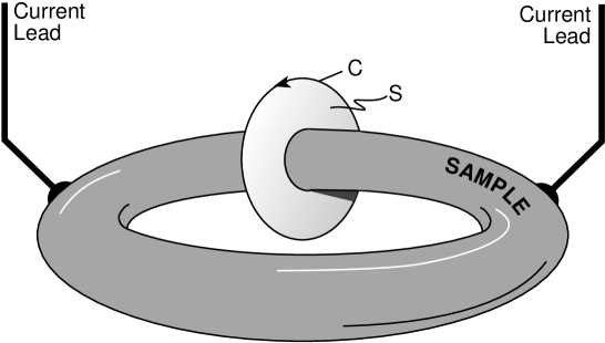
where is the local normal to . In a d.c. transport experiment, where , the currents and will be independent of the particular surface chosen. This argument applies equally well to a singly- or multiply-connected sample including the case where threads a hole in the sample, as in Figure 1. In the case of a two-dimensional sample, the surface becomes a curve traversing the sample, while and are the total currents across the curve.
In the remainder of this section, we shall apply the above considerations to the general hydrodynamic description of an electron system in a strong magnetic field. Our goal is to obtain some relations among the various transport coefficients – both for the transport currents and and for the total local currents, and . We also relate the transport coefficients to microscopic expressions involving correlation functions for currents in the equilibrium state.
Our strategy can be best illustrated by considering a simple example where the electrons are subject to a weak external potential , while the temperature is maintained constant, say by contact with a substrate. Then inside the sample we may write
| (15) |
where is the local chemical potential for the electrons, and and are second-rank tensors, which we denote “transport coefficients.” In thermodynamic equilibrium, the electrochemical potential is independent of position, and , by definition is zero. Since this must be true for arbitrary , we immediately obtain the “Einstein relation” .
Macroscopic equations for the response of the system to a time-dependent perturbation are obtained by combining (15) with the conservation law . (Recall that .) If there is a periodic disturbance in with a wave vector , then the electron density will relax towards the equilibrium state, with const, at a rate , where the diffusion constant is given by
| (16) |
(Again, we assume short-range interactions between the electrons, so is finite for .) A microscopic expression for can be obtained by using quantum mechanics to calculate the response of the system to an infinitesimal time-dependent perturbation , applied at a frequency which is small compared to microscopic frequencies , but high compared to , so that the density does not have time to change significantly. One thus obtains an expression for in terms of a two-time correlation function for fluctuations in in the equilibrium state.
In order to generalize this procedure to the case of non-uniform temperature, we follow the work of Luttinger[13] which involves the introduction of a fictitious “gravitational potential” , which enters the Hamiltonian through its coupling to the energy density. If linear response to is calculated, the response to a temperature gradient may be obtained from the Einstein relations. Our situation is more complicated than the case considered by Luttinger, however, because the Einstein relations apply only to the transport currents, and not to the total currents.
B Current Operators in the Presence of Electrical and Gravitational Fields
The linear response to mechanical fields (electrostatic and gravitational) in a quantizing magnetic field has been presented previously[8]. However, since it is important to the rest of our discussion, we shall review this here. We consider a Hamiltonian of the form
| (17) |
where is the magnetic vector potential, is the scalar potential energy including the confinement and disorder potentials and the periodic potential of atomic cores, and describes the interparticle interactions. Following Luttinger, we introduce the number and energy density operators[13, 15]
| (18) | |||
| (19) |
where , is defined in equation (17), and the curly brackets indicate the anticommutator, .
We are interested in the response of the current-density to time varying external “electrostatic” and “gravitational” potentials and , respectively. These fields couple to the number and energy densities according to the Hamiltonian
| (20) | |||
| (21) |
[We call the function defined by Eqs. (20) and (21) the “gravitational potential” to follow the terminology of the original work by Luttinger[13], although the true gravitational potential would also be coupled to the mass density rather than just to the first-order term of the relativistic energy expansion.]
The conservation laws for energy and particle number imply that the Heisenberg equations of motion for and , under the Hamiltonian , may be written in the form[13]
| (22) | |||||
| (23) |
where and are here operators for the particle and energy currents. The second term on the right-hand side of (23) occurs when there is a time dependence to or . The above equations constrain, but do not determine uniquely, the forms of the operators and , as we may in principle add to them an arbitrary function whose divergence is identically zero. A requirement of strict locality for the particle current, however, together with Eqs. (20) and (21), imposes the form
| (24) |
where is the particle current for :
| (25) | |||
| (26) |
The requirement of strict locality cannot be applied either to the energy current or the energy density in a non-relativistic theory with interactions of non-zero range. However, the form of the energy current is adequately restricted for our purposes if we require that it depends only on the positions and velocities of particles in a small neighborhood of . Although various forms of the energy current may still be written down, which are consistent with this requirement and with a requirement that Eq. (23) be satisfied exactly on the microscopic scale, we shall adopt here the particular definitions
| (27) | |||
| (28) | |||
| (29) | |||
| (30) |
where is the force on particle due to its interaction with . We note that by definition is the energy current associated with the unperturbed Hamiltonian , and equation (27) is valid to first order in , with the requirement that and vary very slowly in space compared to the range of the interaction . It is not difficult to show, under these circumstances, that exactly satisfies the Heisenberg equation of motion (23). To demonstrate this, it is convenient to integrate Eq. (23) over a small volume , and to write the integral of as an integral over the surface of the volume. We also note that
| (31) |
where , if particle is inside the volume enclosed by , and zero otherwise.
With our definitions, the contribution to the energy current from the interaction potential is distributed along the straight-line segment joining and , similar to the distribution of the energy current adopted in Ref. [16]. By contrast, in Ref. [13], Luttinger employed a different form for , where the energy current is supposed to be localized at the two points and . Luttinger’s expression is only approximate on the microscopic level, since it does not strictly satisfy Eq. (23). Our more precise formula and Luttinger’s are equivalent, however, when integrated over any volume large compared to the range of . In fact, in the present paper we have no real need for a precise form for , but will only make essential use of (27).
C Thermodynamic Equilibrium
We first consider the situation of thermodynamic equilibrium. A grand-canonical ensemble, for the perturbed Hamiltonian may be described by a density matrix
| (32) |
where and are Lagrange multipliers, which we may describe, respectively, as the “electrochemical potential” and the “inverse thermodynamic temperature.”
The properties of are particularly simple in the case where and are constants, independent of position. Then the eigenstates of are the same as the eigenstates of , and the density matrix is identical to a density matrix , of the form
| (33) |
with
| (34) | |||
| (35) |
We denote as the “internal temperature,” and as the “internal chemical potential”. The internal energy density and the particle density are the same in the two cases, as is the entropy . Note that and may depend on position, even in equilibrium, if the materials parameters vary in space.
The particle and energy currents are not the same in the two cases, however, because the operators themselves are modified by the presence of and . Using (24) and (27), we see that
| (36) | |||||
| (37) |
The expectation values on the right-hand side represent the particle and energy currents in the “unperturbed” state, with , temperature , and chemical potential . [Note: in Eq. (37), as in Eq. (27) we have dropped terms of order , since we always consider to be small.]
The currents in Eqs. (36) and (37) are purely magnetization currents, since the transport currents vanish, by definition, in equilibrium. In the case of a uniform sample, the magnetization currents are confined to the boundaries. More generally, they are given by Eqs. (3) and (4). This implies that in the equilibrium state, with constant and , we have, to first order in the perturbations, at any point in the sample
| (38) | |||||
| (39) |
where and are the unperturbed magnetizations, (corresponding to ), which we have written explicitly as functions of the chemical potential and internal temperature . (The functions and are also implicitly functions of the material parameters, such as chemical composition and impurity concentration, in the neighborhood of the point .)
The results (34,35,38,39) can be generalized to the case when and vary in space. Equation (32) is still valid in this case. If the length scale of the variation is sufficiently large, the entire system can be considered, within the standard approach, as consisting of small subsystems weakly interacting with each other at imaginary borders. Each of these subsystems, if allowed, will reach a local equilibrium state which depends on the local values and . We assume, of course, that the magnetic field is constant. One can then introduce local thermodynamic parameters (chemical potential, temperature, entropy density, etc.) which are functions of the two independent variables, and . The values of extensive thermodynamic parameters will be then given by the integral of the corresponding local densities over the sample area. In particular, for the total energy, total entropy and total number of particles we have
| (40) | |||||
| (41) | |||||
| (42) |
where , the local entropy density, is the same function of and as for a uniform system. The accuracy of this approximation is limited by terms , which reflect the interaction between adjacent subsystems.
It is more convenient to choose, instead of and , a local “internal” temperature and chemical potential as independent thermodynamic variables. Following Luttinger, we define these parameters in the same way as it is conventionally done for a homogeneous system
| (43) |
[Of course, these definitions are consistent with the thermodynamic relation (9), interpreted in a local sense, with and fixed.]
The equilibrium state defined by the density matrix (32) is the state which maximizes the functional . Using (40), (41) and (42), and setting the variational derivatives of equal to zero, we find
| (44) | |||
| (45) |
which is the generalization of (34) and (35) to the non-uniform case. The equilibrium conditions may be alternatively written as
| (46) | |||
| (47) |
where is the unperturbed temperature of the sample. If is replaced by the perturbed temperature , these conditions reduce to the conditions for thermal equilibrium obtained by Luttinger[13], which are valid for small changes in and .
We now consider the magnetization currents. By definition, the transport currents vanish in an equilibrium state, so the magnetization currents are the total local currents in that case. If , , and vary sufficiently slowly in space, it is clear that and will be still given by Eqs. (38) and (39), provided that the arguments and of the functions and are evaluated at the position . (Corrections will be at least second order in the gradients, if one is away from the boundary of a sample.) Then using Eqs. (3) and (4), for a sample with uniform chemical composition, far from the boundaries, we find
| (48) | |||||
| (49) |
to leading order in and . There will also be additional magnetization currents at the boundaries, given by Eqs. (5), (6), (38) and (39).
D Non-Equilibrium States
We now consider the non-equilibrium situation, where Eqs. (46) and (47) are not satisfied and where , , , and may be in general time-dependent. The local temperatures and are defined to be the same functions of and as in the equilibrium case. We continue to define the magnetization currents and magnetizations by (38), (39), (48) and (49), and we define the remaining contributions to the currents to be the transport contributions.
By the locality hypothesis, the transport currents must be given by a sum of terms proportional to the gradients , , and , in the limit where the applied fields are small. Our aim is to determine the coefficients of these terms. The requirement that the transport currents vanish when (46) and (47) are satisfied means that the gradients enter only in the combinations and . This observation is the generalization of the “Einstein relation” to the case in which there is a non-uniform , and allows the response to the statistical fields and to be related to the response to the mechanical fields and .
To determine the remaining unknown coefficients, we consider a particular situation, where the potentials and vary periodically in time, with a characteristic frequency small compared to the microscopic relaxation rate but large compared to the size-dependent relaxation rates for the energy and particle density. (This is the “rapid case” of Ref. [13].) In this situation the local values of and are not changed from their initial values, so that and remain constant throughout the sample.
We concentrate on a region far from the boundaries. Since , we may write the total currents as
| (50) | |||||
| (51) |
with transport coefficients that can be expressed in terms of time-dependent correlation functions in the framework of the standard Kubo formula[13]:
| (52) | |||||
| (53) | |||||
| (54) | |||||
| (55) |
Here the subscript 0 on each time-dependent current operator and indicates the limit of its spatial Fourier transform, and the angular brackets denote the quantum mechanical and thermodynamic average in the equilibrium state of an infinite system at temperature and chemical potential .
In order to find the transport currents when , we subtract from (50) and (51) the bulk magnetization currents, given by (48) and (49). We thus find
| (56) | |||||
| (57) |
where is the unit antisymmetric three-tensor: if the is an even (odd) permutation of , and zero if two indices are equal. By definition, transport currents flow only in the bulk of the sample. To simplify notation, we have therefore dropped the label “bulk” in the above equations, and will do so for all subsequent transport current densities.
Now we can consider the general case, for an arbitrary value of , where , , , and may be all non-zero. As remarked earlier, the condition that the transport currents vanish in equilibrium requires that the gradients enter only in the combinations and . (In other words, the Einstein relations, extended to the case where and are different from zero, apply to the transport currents in the presence of finite magnetic field.) Thus we have, in the general case:
| (58) | |||||
| (59) |
Of course, (58) and (59) reduce to the Luttinger formulae[13] when the magnetic field is absent, so that .
To obtain the local currents, in a uniform sample far from the boundaries, in the general case where , , and are all independent, we must add the magnetization currents, given by (48) and (49) to the transport currents given by (58) and (59). In addition, there will be boundary currents from the magnetization. In the absence of the fictitious gravitational potential the change in the integrated boundary currents at a point , Eqs. (5) (6), is determined by the changes in the temperature and chemical potential at that point, according to
| (60) | |||||
| (61) |
Although we have introduced the fictitious field to derive linear response, we will have no further need of it, and hence shall set for the remainder of this paper.
It is convenient to introduce the electrochemical potential, defined by
| (62) |
An ideal voltmeter, (with leads that have no thermopower) will measure the difference in between two contact points. In a thermodynamic equilibrium state, the value of , as well as the temperature , will be constant throughout the system.
It is also convenient to define a transport heat current density as
| (63) |
Then we may rewrite (58) and (59) in the form
| (64) | |||||
| (65) |
where
| (66) | |||||
| (67) | |||||
| (68) | |||||
| (69) |
Although our derivation has assumed to be infinitesimal, the final results for the transport currents, given by (62)–(69) and (52)–(55) are written in a form that remains valid when is not small. This accounts for the slight differences (which are beyond leading order in the driving fields) between the above coefficients, , and those obtained by direct substitution of Eqs. (58) and (59) into Eq. (63). When is not small, the expressions (50) and (51) should contain additional higher-order terms in ; the coefficients appearing above cannot therefore be defined by these expressions, but are assumed to be defined by the Kubo formulae (52,53,54,55). In the case of finite , equation (49) for the bulk magnetization current must also be modified by the addition to the right-hand side of a term ; the edge current is still given by (6) and (39).
E Onsager Relations
The transport coefficients for and , given by (64)–(69), obey Onsager symmetry relations[17, 18] of the form
| (70) | |||||
| (71) | |||||
| (72) |
To see that this is the case, we first establish that the coefficients obey Onsager relations of the same form as (70)–(72). This follows from the expressions relating to the current correlation functions, (52)–(55), and the invariance of the Hamiltonian under simultaneous reversal of time and magnetic field. Secondly, we note that the magnetizations and reverse sign under reversal of . Equations (70)–(72) follow directly.
In contrast the local current densities do not satisfy the Onsager relations. The local current densities differ from the local transport current densities by the bulk “magnetization currents”. These additional magnetization contributions to the local response in general depend on which driving field is applied (e.g. whether it is or ), and give rise to a set of transport coefficients, one for each driving field, which differ by terms proportional to the gradients of magnetization densities. Since no general symmetries relate these additional magnetization terms, neither the Einstein relations nor the Onsager relations hold locally for the total current response.
As a specific example, consider the local bulk currents and in terms of and , under conditions where . By combining (63)–(69), with (1), (2), (48) and (49), one may readily obtain expressions for the appropriate coefficients
| (73) | |||||
| (74) |
As far as we are aware, there is no symmetry relating the derivatives of and with respect to and , so these coefficients apparently do not satisfy the usual Onsager relations.
Moreover, if we consider instead a situation where , but , we find according to (50) and (51), . This coefficient, which is different from , is also clearly not related to by Onsager symmetry in the general case.
Although the contribution of the magnetization current does not appear in standard transport experiments, the local electric current distribution is measurable, at least in principle, by a sufficiently sensitive measurement of the magnetic field generated by currents in the sample. Since the magnetization current does not dissipate Joule heat, it could not be detected using the well-known technique based on local luminescence intensity[19]. Measurements of the local electric field distribution by means of the electro-optic effect[20] do not serve this purpose either, since the magnetization current is related to the “statistical fields” and rather than to the electric field . In the case of the energy current or heat current, we are not aware of any reasonable method for direct measurement of the local currents.
We illustrate our results further with the example of the number current for a two-dimensional electron system with no disorder, at a Landau-level filling fraction for which the electron system is incompressible at . At the filling fraction , we have . Then we have
| (75) |
where the last equality follows from the incompressibility condition for . Here is a unit vector directed upward from the plane.
The coefficient for this system is given by the Hall conductivity: . On the other hand, substituting into Eqs. (1), (48) and (58), we see that the coefficient describing the local response to vanishes, and all number current flow in the bulk is due to the electric field: . The current driven by an inhomogeneous chemical potential is localized at the edge, and is given by , where is a unit vector in the plane, perpendicular to edge, in the outward direction.
F Inhomogeneous Samples
Although we have concentrated so far on the case of a homogeneous sample with boundaries that are sharp compared with the overall length scale, it is easy to generalize our results to the case of a sample whose material parameters, such as chemical composition, vary on a macroscopic length scale. The formulae (64) and (65) still hold locally for the transport currents in this case, with the qualification that the transport coefficients depend on the local material parameters, and can therefore vary from one place to another in the sample. The magnetization currents at the boundary of the sample are still given by (60) and (61), with the qualification that the functions and may also vary from one place to another because of their implicit dependence on the local material parameters. The magnetization currents in the bulk of the sample are no longer given simply by Eqs. (48) and (49) however. If we denote the material parameters by a set of variables , and we set , then (48) and (49) should be replaced by
| (76) | |||||
| (77) |
[These expressions follow directly from (3), (4), (38) and (39).] In the quantities and , which appear in (76) and (77), it is necessary to keep not only the zeroth order terms, but also the first-order changes engendered by the deviations and .
G Long-Range Forces
The derivation in the previous subsections, and various intermediate results, require modification when there are long-range forces due to unscreened Coulomb interactions. In two-dimensional structures, this is the case when the metallic gate is either absent or is situated farther than the characteristic length scale of the fields applied.
If uncompensated electric charges are present, there can be energy transport over long distances via the macroscopic electric field, and the total energy current at a given point of space does not, in general, depend solely on the state of the particle system in the immediate neighborhood of that point. Moreover, the convention of Eq. (28), in which the interaction contribution to the energy current is concentrated along the line-segments joining each pair of particles, is not generally used in this case.
The most convenient approach is to break up the interparticle interactions into a long-range piece, mediated by the macroscopic electric field , and a short-range piece, which includes everything else. The macroscopic field is supposed to be averaged over a region sufficiently large that fluctuations in the field, arising from thermal or quantum fluctuations in the microscopic electronic charge density, can be neglected. Thus there is no entropy transport via the macroscopic field. As a result, we find that with appropriate definitions we can write local hydrodynamic equations for the heat current and particle current which are similar in form to the equations derived for short-range forces. (We assume here that we are working at a temperature sufficiently low that heat transport via the radiation field may be completely neglected. Formally, this assumption is imposed by taking the limit where the speed of light is infinite.)
To make these points clearer, we note that since charge is locally conserved, charge fluctuations with the longest range effects are electric dipole fluctuations. In the absence of the radiation field, the interaction between dipoles at two different points falls off as the inverse cube of the separation, and the rate of energy transfer due to random thermal motion would be expected to fall off as the inverse sixth power of the separation. At large distances this process will be much slower than the conventional process of heat conduction (already taken into account in our discussions) wherein energy is transported diffusively via a series of many short jumps.
To proceed formally, we redefine the interaction appearing in subsection B to include only the short-range part of the Coulomb interaction, after effects of the macroscopic electric field are subtracted out. First, we choose a truncation radius which is much larger than the average inter-particle distance but much smaller than the macroscopic scales of external fields and, if the sample is not uniform, the scale of the equilibrium density variation. We split the Coulomb interaction potential into the sum of two terms, , where decays rapidly at , and contains the long-range tail of the interaction and changes smoothly at distances . Then we replace by in the definition of and , Eq. (17), and include the long-range component in the self-consistent macroscopic field .
We continue to define by Eq. (19), and define the internal energy density as the expectation value . Then may be interpreted as the matter contribution to the energy density. The total energy (with ) is then given by
| (78) |
where is the dielectric constant of the background material, and we assume the background magnetic permeability is unity. The energy current will similarly be broken up into two parts
| (79) |
where the second term is the standard contribution from the macroscopic electromagnetic fields, and , which we may think of as the matter contribution to the energy current, is defined by Eqs. (28)–(30), with replaced by in the definition of . Of course, and are determined self-consistently from the macroscopic current and charge distributions using Maxwell’s equations in the static limit. Equations (78) and (79) are asymptotically correct in the limit where is large compared to the microscopic scale but small compared to the scale of variation of .
For a two-dimensional electron system in an external magnetic field, the magnetic fields arising from currents in the sample are generally very small, and may be omitted from the term in Eq. (78). Thus this term is independent of the state of the electron system and may be ignored if desired. On the other hand, the magnetic fields generated by the currents in the sample must be included in the second term on the right-hand side of (79), because the speed of light appears as a prefactor. Note also that and are restricted to the two-dimensional layer, but the electromagnetic contributions to (78) and (79) extend into the space outside. Below we focus on the matter part of the energy current.
It is now possible to redo the arguments of the previous section with little modification. We restrict our attention to the situation where the applied magnetic field is independent of time and assume that the macroscopic electric field may be derived from a scalar potential
| (80) |
The potential is obtained self-consistently, and includes effects of any macroscopic time-dependent variations in , as well as the effects of any static charges present in equilibrium and the external perturbations embodied in . In general, we cannot consider that is infinitesimal, even in equilibrium.
In order to repeat our previous derivations, one needs to consider a non-zero gravitational potential ; we present here the final result, and hence set . We redefine the electrochemical potential as
| (81) |
The definition (27) of the energy current in the perturbed system is now replaced by
| (82) |
where is the particle current density, and was defined above. As we did in previous sections, we split the local currents and into magnetization and transport parts, and we define a transport heat current as given by Eq. (63). Then and obey equations identical to (64)–(69), with defined by Eqs. (52)–(55) in terms of the correlators for the matter currents and under the Hamiltonian for a uniform system in equilibrium, with . The transport coefficients obey the same Onsager relations as before.
Note that different definitions of the macroscopic electric field, as may be obtained by different choices of the truncation radius , will generally cause an exchange of contributions between the chemical potential and the electrostatic potential . This will also transfer contributions between the first and second terms in Eq. (82), leaving the sum unchanged. As long as the different values of remain sufficiently large, the change in the truncation should not affect the coefficients since the correlators in Eqs. (52)–(55) are sensitive only to short-range properties of the system.
We also note that in realistic two-dimensional systems, the component of the electric field perpendicular to the electron layer, arising from charges on gates or from ionized impurities displaced from the layer, may play an important role in confining the electrons to the layer. It is therefore important to include this part of the macroscopic electric field in the unperturbed Hamiltonian and in the definition of the energy current when calculating the correlation functions that appear in (52)–(55). Formally this can be done by including the perpendicular confining field in the one-body potential which enters Eq. (17), and excluding it from the macroscopic potential . Then the equilibrium is a constant in the direction perpendicular as well as parallel to the layer, and can be safely omitted from . In fact, it may be convenient to include the entire equilibrium value of the electrostatic potential in , even in an inhomogeneous system, so that describes only long-wavelength fluctuations about equilibrium.
H Additional Remarks
Throughout this section, we have treated the fields , , and (or , in subsection G) as independent variables, which can be arbitrary functions of position, subject to the constraints that gradients are small, and that and are infinitesimal. (The fictitious field was set equal to zero in the latter part of the section.) The transport currents depend on gradients of and (or ) only through the combination . In a d.c. transport experiment, there are strong additional constraints arising from the requirements that the currents must be divergence-free in the interior of the sample, and must satisfy appropriate constraints at the boundaries. Typically, these conditions completely determine the spatial variations of and throughout the sample interior, when boundary values of the fields are specified, or when current flows through the boundaries are given.
For the case of a two-dimensional electron system on a three-dimensional substrate, the situation is slightly more complicated. We shall be concerned with situations where the substrate is an electrical insulator, so that the divergence of the two-dimensional electric current is required to be zero in the analysis of experiments. On the other hand, we consider the thermal coupling to the substrate, via absorption or emission of phonons, to be small but not zero. Then on length scales large compared to , where is the electron-phonon relaxation time and an appropriate thermal diffusion constant for the isolated electron system, the divergence of is not necessarily zero. Instead, one should take the value of to be an independent variable determined by conditions in the substrate.
Although our previous discussions assumed the sample to be isolated from its environment except at its edges, the transport equations derived above should remain valid provided the electron-phonon coupling is sufficiently weak that is large compared to the microscopic times necessary to establish local equilibrium in the electron system.
In order to calculate the transport currents, it is not generally necessary to find the separate portions of arising from and from the electric field. This is necessary, however, if one wishes to obtain the local current distribution. In practical situations, where the nearest external conductor is far from the electron layer compared to the mean spacing between electrons in the layer, the value of will be relatively small compared to the value of or . This is due to the fact that, in the absence of external screening, perturbations in and are not really independent and their characteristic magnitudes can be expressed via each other. Suppose that a non-equilibrium perturbation in the chemical potential with a large length scale is created in a two-dimensional system. The resulting variation in the particle density has a magnitude . The magnitude of the potential variation caused by this accumulation and depletion of electrons can be estimated as . Thus, in a compressible system, we find the ratio of gradients to be of the order of which is small in the limit of large . In an incompressible system (for instance, a macroscopically wide strip of a system in the middle of a quantized Hall plateau, if there are no localized states in the energy gap), the accumulation of electrons due to the perturbation in the chemical potential occurs only at the edges of the system. The accumulated charge creates an electric field that slowly (as ) vanishes into the interior of the sample. The resulting ratio is as small as where is the width of the strip[21].
The above observation has an impact on the issue of the edge-versus-bulk current distribution. Since, in the absence of a temperature gradient, the boundary currents arise solely due to , and the bulk currents are due to both and , the non-equilibrium current in a system without gates flows predominately in the bulk. The situation changes, however, if the temperature is not uniform. As we shall see in Sec. IV, the boundary fraction of the net thermocurrent is at least as significant as its bulk counterpart.
III LINEAR RESPONSE IN THE ABSENCE OF DISORDER
In the previous section, the local current response to the electric and statistical fields was expressed in terms of the coefficients of the mechanical response in the bulk defined by the general expressions (52)–(55). Now we derive explicitly three of the four response coefficients for a simple case of a uniform disorder-free sample. Since the internal magnetization currents and the boundary currents are already expressed in terms of the equilibrium magnetizations and their derivatives as given by Eqs. (11,12,81,82), here we consider only the “transport” components of the bulk currents. We restrict our attention to the case of a two-dimensional electron system, with magnetic field in the direction, perpendicular to the layer.
Our main result is the expression for the number current density
| (83) |
which shows that, in the absence of disorder, the transport contribution to the number current density is fully determined by the equilibrium number and entropy densities. (In this section, the symbol represents the two-dimensional antisymmetric tensor .)
Equation (83) is valid locally for any interacting electron system, provided it does not have a shear modulus, i.e., is a fluid, and the energy spectrum of electrons is quadratic. We present two different ways to obtain this result. In Sec. A, we derive Eq. (83), and hence the coefficients and directly, using arguments based on fluid dynamics. In the alternative proof given in Sec. B, we first derive the coefficients and by studying the current response in a uniform electric field, and then obtain from the Onsager symmetry. The advantage of the second derivation is that it deals with a homogeneous non-equilibrium system, .
Both derivations that follow employ the physical notion of internal pressure, which is not quite obvious in the presence of a magnetic field and which we now discuss briefly. In the presence of a uniform magnetic field the equation for conservation of momentum on the microscopic scale may be written
| (84) |
where is the one-body potential and is the internal stress tensor at point . As in the case of the energy current discussed in Section II, there is not a unique definition of for a system with finite range forces. However, a definition consistent with Eq. (84) and with the requirement of quasi-locality is
| (85) |
where is defined by Eq. (29). Equation (85) may be checked by integrating both sides of (84) over an infinitesimal volume, to obtain the rate of change of the momentum inside the volume. The integral of the last term on the right hand side of (84) is equal to the integral of the stress tensor over the surface enclosing the volume. The first term of (85) then gives the change in momentum due to particles crossing the surface, while the second term gives the force exerted on particles inside the volume by particles outside the volume [cf. Eq. (31)].
In applying the above equations to the present problem, we interpret as the band mass rather than the bare mass of the electron, and excludes the periodic potential of the ions. Thus, when there are no impurities present and no applied electric field, is a constant in the interior of the sample, and arises only from the confining potential at the boundaries. We also assume that depends only on the distance between the electrons, so that is parallel to and the stress tensor is symmetric. We specialize to the case of a two-dimensional electron system and thus use notation appropriate to two dimensions.
In thermal equilibrium, far from the boundaries, in an isotropic system, the stress tensor must be proportional to the unit tensor, so we may write
| (86) |
where , the “internal pressure”, depends on the chemical potential and temperature. In the presence of a magnetic field, is not equal to the pressure which appeared in the thermodynamic equations (9)–(12) and which is equal to the force per unit length exerted by the boundaries on the contained electron gas. Rather, we have
| (87) |
The difference between and arises from the Lorentz force exerted by on the boundary current .
Equation (87) may be obtained directly from equations (84) and (86) if we integrate the right-hand side of (84) along a line-segment from a point in the interior of the sample, to a point where , passing through a point on the boundary. Since in equilibrium, and since at point , we find
| (88) |
The right-hand side of (88) is just the force per unit length exerted by the boundary at point . The fact that the pressure entering the thermodynamic equations is indeed the same as the force per unit length exerted by the boundaries follows from the well-known fact that a magnetic field constant in time cannot produce work on charged particles. Hence, although there is a momentum exchange between the system and the source of the field via the Lorentz force, there is no energy exchange at const. Therefore, the term in Eq. (59) represents the work done by the expanding system on the external confinement. To avoid confusion, we note that the work done by the expanding system against the Lorentz force actually goes to increase of the internal energy of the system itself[22].
A Fluid Dynamics Approach
Consider an electron liquid in a uniform magnetic field and in the presence of an electric potential, chemical potential, and temperature all of which vary smoothly in space. All the fields and currents in the system are assumed to be either constant in time or varying at a small frequency as discussed in Sec. II A. We concentrate on a small macroscopic element of the liquid with area in the interior of the sample, which we choose to be of a size much less than the length scales of the fields and much larger than the average inter-electron distance.
Then, setting in the RHS of (84), and setting , as is appropriate for a quasi-equilibrium situation, we find
| (89) |
where , and are averaged over the element . If the induced current is small, then the correction to arising from the current should be second order in , and therefore negligible. Thus may be replaced by its equilibrium value, , evaluated for the local values of and . To first order, Eq. (89) becomes
| (90) |
Apart from the additional term resulting from the pressure gradient, the right-hand side of Eq. (90) represents the classical drift velocity in the crossed magnetic and electric fields. Substituting Eq. (87) into Eq. (90) and using the relation which follows from Eqs. (9) and (10), we finally obtain
| (91) |
where coincides with the right-hand side of Eq. (83), and the second term is the internal magnetization current as defined by Eqs. (3) and (7).
We note that our arguments do not apply to an electron solid. In a solid, a non-uniform drift current will cause a shear deformation which will increase until the stress forces suppress the local drift. Equation (89) determines the force acting on an element of a liquid and does not include the shear stress contribution when we use (86). In addition, the pinning effects which arise in the presence of even a weak disorder potential makes our consideration completely inapplicable in the case of an electron solid.
B Derivation Using Onsager Symmetry
We now study a homogeneous system, , which is driven out of equilibrium by an external electric field . Since we study coefficients of the bulk response, we can assume that the electric field is uniform and the system itself is infinite. In addition to the original laboratory frame, we consider the system in the “primed” reference frame moving at a velocity
| (92) |
in which the applied electric field vanishes. Since the system is homogeneous, and disorder potential is absent, Galilean invariance requires that properties of the system in both reference frames are the exactly same. Due to the absence of electric field in the moving frame, the system with respect to this frame is in equilibrium. The number and energy current densities in this frame are therefore zero, . In the laboratory frame, the system moves as a whole at a velocity . Hence the number current density defined as the average number of electrons passing through unit length per unit time is given by
| (93) |
To determine the energy current density, we split the whole system in two parts by an imaginary straight line perpendicular to the drift velocity and find out how much energy is transferred, in the laboratory frame, from one part of the system to another in time . The energy has two contributions, one from the direct transfer of an element of the system across the line, and another due to the work done by one part of the system on the other part while moving
| (94) |
where is displacement of the system in time , is the length of the line segment which we consider, and is the pressure in the interior of the sample. Substituting Eq. (87) for the internal pressure into (94), for the energy current density we obtain
| (95) |
One can also obtain Eq. (95) directly from the microscopic expression for the energy current, given by Eqs. (27)–(30). Let us write , where is the velocity of particle in the frame moving with velocity . In the moving frame, the system is at local equilibrium with an energy density and a stress tensor . Comparing (28)–(30) with (85), we see that (95) is correct to first order in .
Identifying Eqs. (93) and (95) with the expressions for the bulk current response (50), (51), and substituting from Eq. (92), we find the response coefficients
| (96) | |||||
| (97) |
As one can see from the last formula, is an odd function of the magnetic field. From this fact, and from the symmetry relation discussed in Sec. II E, we have
| (98) |
Substituting the obtained coefficients , , and into (66)–(68), and using (7) and (10), we find , and
| (99) |
Then using (64) we arrive at Eq. (83) for the transport number current.
IV THERMOPOWER MEASUREMENTS
A Thermopower Measurements and Current Distributions
We now turn to discuss the thermoelectric properties of real samples, in which temperature gradients are maintained by the coupling of the electron gas to the phonons of the substrate. To use the results of the previous sections, we shall assume that the sample is homogeneous, and that the coupling to the substrate is sufficiently weak that the corresponding thermal relaxation rate is much slower than the microscopic relaxation rate of the electron gas , and the response of the electron gas is well-described by the transport properties of the isolated electron gas. However, we assume that the thermal coupling to the substrate is sufficiently strong that on a macroscopic scale we may assume that the local temperature of the two-dimensional electron gas is equal to the local temperature of the substrate, and we need not impose the condition that in the electron gas. The substrate is assumed to be an electrical insulator, however, so that in the electron system. We do not discuss the energy current in this section.
A convenient way in which to study the thermoelectric response of a sample is through the thermopower. A thermopower measurement involves the application of a uniform temperature gradient to a sample which is disconnected from current leads. Since there can be no average electron current flow, an electrochemical potential gradient develops. The thermopower tensor is defined in terms of this potential gradient.
If the diagonal matrix elements of and are different from zero, it can be shown that the conditions , with at the sample boundaries, together with Eq. (64), require that everywhere. This is the case only if
| (100) |
everywhere in the sample, where
| (101) |
In the special situation where and are proportional to the antisymmetric tensor , as occurs for instance in the case of zero impurities, the value of is not properly determined by the conservation equations, together with Eq. (64) and the boundary conditions. For example, one may add to any function which vanishes at the boundaries of the sample, without affecting the values of in the interior or at the boundary. The average value of is still given correctly by Eq. (100), however, for any solution of the equations, and the value of at any point of the boundary will be the same as if were uniform in the sample. Thus the experimentally measured thermopower, in which the voltage drop is measured between two points at the boundary, would still be given by Eq. (100) in this case.
For the remainder of this section, we will focus on the thermopower of systems in which the disorder potential is weak. In the limit of vanishing disorder, one can use the response coefficients we have derived in the previous section, and the thermopower tensor takes a particularly simple form
| (102) |
Thus, the thermopower tensor is diagonal, with a magnitude given by the entropy per particle, , divided by the charge per particle, . This result is familiar for non-interacting electrons[3, 6, 7].
Unfortunately it difficult to provide a general criterion for how weak the impurity scattering must be in order that its effects on the thermopower can be neglected and Eq. (102) applies. Rather, the form of such a criterion depends on the nature of the low-lying charged excitations of the system, which may be quite different at different filling fractions (compare, for example, filling fractions at which the system is compressible and incompressible in the zero-temperature limit). A necessary condition for Eq. (102) to apply is that the impurity scattering is sufficiently weak that both of the tensors and are almost purely off-diagonal, such that the thermopower tensor itself is close to diagonal. In some circumstances this condition may not be sufficient, as there may be corrections to the size of the diagonal thermopower. The form of such corrections depends on the specific experimental conditions, and requires a specific calculation of the effects of impurity scattering on the carriers. In the following, we will concentrate on thermopower of systems for which the impurity scattering is sufficiently weak that Eq. (102) applies. In the next subsection we will discuss the form of the corrections that can arise due to impurity scattering for filling fractions close to or .
Although, under the conditions of the experiment, no net current passes through the sample, in a quantizing magnetic field circulating non-equilibrium currents are induced. In the bulk, these are internal magnetization currents, whose continuity at the edge is provided by the boundary currents. As we shall now show, these currents can be very large, in the sense that the local current density in the presence of both the temperature gradient and the compensating electric field can be comparable to what it would have been in the presence of only one of these fields.
Let us compare the average and the local current densities induced by a uniform temperature gradient alone, const, with . We consider a filling factor which is an important and much studied example of a compressible state. The average current density is equal to the transport current density (83)
| (103) |
The portion of this current that flows in the bulk is given by
| (104) |
where we used Eq. (48) and the thermodynamic relations (9)–(11).
In a strong magnetic field, for which all electrons are restricted to the lowest spin-polarized Landau level, one may express the entropy per unit area in the form , where is the number density of flux quanta, is the entropy per flux quantum, is the filling fraction, and we have assumed a Coulomb force-law, for which the typical energy scale is set by the magnetic length, . Using , one can write
| (105) |
Now, at a filling fraction of one half, particle-hole symmetry requires that . Hence Eq. (104) may be rewritten
| (106) |
We shall discuss two cases.
First, for an ideal non-interacting electron gas (for example ), the entropy is independent of the temperature at fixed filling fraction, so the above expression is identically zero. The temperature gradient induces no number current in the bulk of the system, and all of the induced current flows around the edge of the sample.
Secondly, for a system interacting by Coulomb forces, the entropy at is believed to be approximately linear in temperature (with a logarithmic correction at very low temperature due to the divergence of the effective mass of composite fermions)[23]. The bulk current induced by the temperature gradient is therefore approximately , which is one half of the total current induced by the temperature gradient (103); the remaining current flows around the edge of the sample.
In both of the above cases the current driven by the temperature gradient is found to be very inhomogeneous, with all or half of the total current flowing on the edge of the sample.
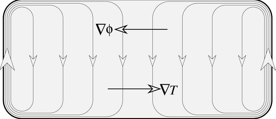
In contrast, the distribution between edge and bulk of the current driven by in a thermopower experiment depends on the apportionment between and . The relative proportions of coming from and depends on the compressibility of the electron system and on the electrical capacitance per unit area, i.e., on the distance to the nearest conductivity surface. In most practical cases, the contribution of will be much larger than , so that , and . In this case, the compensating current driven by will be uniformly spread over the sample and a strong circulatory current is set up by the combination of and . The non-equilibrium part of the current density induced by the thermopower measurement has a form shown schematically in Figure 2.
B Experimental Comparison
Finally, we will compare our conclusions concerning the thermopower of a sample in the limit of weak disorder with recent thermopower measurements in the fractional quantum Hall regime. At high temperatures, the observed thermopower is dominated by the phonon-drag contribution resulting from the momentum exchange between the system and the phonons in the substrate. Very low temperatures are required before the intrinsic thermopower caused by the diffusion and drift in the system itself can be observed. It is only very recently that this has been achieved in the fractional quantum Hall regime. In Ref. [11, 12], thermopower measurements on a hole gas in this regime are reported, and it is found that at temperatures below about 100 mK the intrinsic thermopower can be distinguished. The crossover from a dependence of the thermopower at high temperatures, to a linear temperature-dependence below 100 mK is associated with the transition from phonon-drag-dominated to diffusion-and-drift thermopower. At such low temperatures the signal-to-noise ratio is rather poor in thermoelectric measurements, so it is difficult to resolve much structure related to the incompressible states at fractional filling fractions. One can, however, distinguish dips in the diagonal thermopower, , at , 2/5, 3/5, 2/3, consistent with the expectation that the thermopower should vanish at these filling fractions for which the entropy is exponentially small.
A more interesting issue is the behavior at even-denominator filling fractions. It is found that exhibits a broad maximum at and, less clearly, at . As explained in Ref. [11] the absolute values of the thermopower are inconsistent with a single particle picture, and electron-electron interactions must be considered.
It has been argued that, at even denominator filling fractions, the appropriate description of the electron system is in terms of a Fermi liquid of weakly interacting composite fermions[23]. We will use this model in conjunction with equation (83) to calculate the thermopower of a disorder-free system. Let us first assume that electrons are maximally spin-polarized. Thus, we assume that at a filling fraction of , the lowest (spin-split) Landau levels are filled (and therefore contribute zero entropy), and that the remaining half-filled Landau level may be represented by a Fermi liquid of composite fermions with effective mass . The entropy of the half-filled level is determined by the density of states at the Fermi surface, so we obtain the thermopower of the system to be
| (107) |
where the particle charge is for electrons and for holes. Note that the same formula applies at all half-integer filling fractions . However, one must be careful to use the appropriate value for the effective mass, which may vary for different absolute magnetic fields and for different filling fractions .
Corrections to Eq. (107) due to impurity scattering may arise if the scattering rate of the composite fermions from impurities is larger than the microscopic equilibration rate of the disorder-free composite-fermion system. Since this equilibration rate becomes very small for composite fermions close to the Fermi surface, it may well be the case that in experiments at low-temperature the impurity scattering rate is sufficiently large, , that corrections to Eq. (107) arise. Arguments based on a Boltzmann transport theory for the composite fermions suggest that, in this case, impurity scattering will affect the thermopower (107) if the scattering rate is energy-dependent[24]. Specifically, if we consider a model of composite fermions with conventional parabolic dispersion, , and a transport scattering rate that varies with energy as , then the effect of impurity scattering is to multiply Eq. (107) by a factor :
| (108) |
This has the same form as the conventional Mott formula for the thermopower of a spinless two-dimensional electron gas in zero magnetic field[10].
A calculation[25] of the scattering of composite fermions in modulation-doped quantum wells suggests that it is only weakly energy-dependent, , and the corrections to (107) are small. In the following, we will compare the experimental observations with Eq. (107), bearing in mind that a prefactor may arise due to impurity scattering.
Comparing Eq. (107) with the measurements of reported by Ying et al.[11], we find that, at a filling fraction of and at a magnetic field , an effective mass of is required for consistency, where is the free-electron mass. This value is a factor of 2 larger than the value obtained in Ref. [11] from their own analysis of the data, which used the Mott formula Eq. (108) with an assumed value of . However, our value of the effective mass does not seem inconsistent with estimates of based on other types of transport measurements. For example, a value of at is quoted in Ref. [11] for a hole doped sample with a higher carrier density, such that occurred at . In an ideal system, with no Landau-level mixing, zero layer thickness, and no impurity corrections, the effective mass at would be expected to be proportional to , which would predict a value for the sample used for the thermopower measurements, where occurred at . However, it is not at all clear that this scaling should apply to the actual samples. (The observed value of the effective mass at is in any case considerably larger than one would expect based on numerical studies of finite systems where Landau-level mixing, finite thickness, and impurity effects are ignored.)
We note that the value assumed in Ref. [11] was obtained from calculations of impurity scattering of electrons in zero field, whereas calculations[25] for composite fermions suggest a much smaller value , as was mentioned above.
The difference between our formula and the one used in Ref. [11] is much more serious at . In that case Ying et al.[11] replace the particle density in Eq. (108) by the density of composite fermions, which is now 3 times smaller than the density of holes in the valence band. We, believe, however, that whether one uses Eq. (107) or Eq. (108) the quantity should be the total number of carriers, including those in any filled Landau levels.
Since the experimental thermopower reported in Ref. [11] is larger at than at by a factor , Ying et al. conclude that , which they view as evidence for the validity of a model of spin-polarized composite fermions at . However, we would conclude using Eq. (107) or Eq. (108) that . This is contrary to the expectation for the ideal system that should be smaller than , due to the smaller value of .
Unfortunately, we do not see any justification for the analysis used by Ying et al. at . We believe that our starting formula (107) is correct in the limit of small impurity scattering, and that energy-dependent impurity scattering leads to an additional prefactor that is close to unity. Moreover, the relation holds even allowing such impurity scattering, provided the exponent is the same at each filling fraction. (In the absence of any Landau level mixing this would necessarily be the case if the magnetic length were the same at each filling fraction. The change in magnetic length by a factor of that occurs between and at fixed electron number density is unlikely to affect the exponent .)
It therefore appears to us that the reported thermopower measurement at are not consistent with a simple model based on spin-aligned composite fermions. The failure of this model may be due to the combined effects of increasing degree of Landau level coupling and the smaller Zeeman energy expected at as compared to . Alternatively, the effects of disorder may be quite different at these two filling fractions. Neglecting any significant effects of disorder, however, and viewing the diagonal thermopower as a measure of the entropy, one would conclude that the entropy at is larger than what one would expect from a model of maximally spin-polarized composite fermions. It may be that additional entropy arises from the loss of spin-polarization. A number of experiments indicate that in typical electron doped GaAs samples, the electron system is not maximally spin-polarized at even at [26, 27, 28, 29]. It is not clear whether this will also occur for hole-doped samples, where the Zeeman energy may be more important due to the larger g-factor. To gain better understanding of the origin of the discrepancy at , it would be interesting to investigate the dependence of the thermopower on the extent of Landau level coupling (e.g., by studying -type samples, or -type samples with different densities), and on the Zeeman energy (by tilted field measurements).
V Conclusions
We have discussed the linear response of a homogeneous, bounded interacting electron gas in quantizing magnetic field. We studied the number and energy currents which arise in response to the gradients in electric and chemical potential and in temperature. We derived general expressions for the bulk and boundary currents in the presence of mechanical and statistical fields. In general, the boundary of the sample can carry a finite fraction of the total current passing through the sample. The local response in the bulk may be described as a sum of “transport” and “internal magnetization” contributions. Internal magnetization currents do not contribute to the net current, are always divergenceless, and cannot be revealed in any standard transport experiments performed on either homogeneous or inhomogeneous samples. They can be detected only in special contactless experiments resolving the local current distribution. We found that Onsager symmetry relations cannot, in general, be applied directly to the local current densities in the bulk of the sample. However, they do hold locally for the transport currents, and therefore for the net currents passing through the sample. We derived expressions for three of the four response functions of an interacting system in the limit of weak disorder in terms of equilibrium properties of the system. In particular, we showed that, in this case, the thermopower tensor is diagonal and is proportional to the entropy per particle. Recent thermopower measurements on a high-mobility sample show that this conclusion is consistent with a model of a Fermi liquid of spin-polarized composite-fermions at . However, for the observations to be consistent with this model at , a very large effective mass is required. An effective mass of this size seems unlikely, and we suggest that the spin-polarized composite-fermion state may not be a good description of the system at that filling fraction.
ACKNOWLEDGMENTS
The authors are grateful to M. Shayegan for originally stimulating their interest in this problem, and for helpful subsequent discussions. We would also like to thank P.N. Butcher for helpful comments, and D.V. Khveshchenko for providing us with Ref. [25] prior to publication. This work has been supported in part by NSF grant DMR94–16910 and in part by the NATO Science Fellowship Programme.
REFERENCES
- [1] Present address: Institut Laue-Langevin, B.P. 156, 38042 Grenoble, Cedex 9, France. [cooper@ill.fr]
- [2] Present address: Department of Molecular and Microbiology, Tufts University, Boston, MA 02111.
- [3] Y. N. Obraztsov, Fizika Tverdogo Tela 7, 573 (1965), [Sov. Phys. Sol. State 7, 455 (1965)].
- [4] S. M. Girvin and M. Jonson, J. Phys. C 15, L1147 (1982).
- [5] P. Streda, J. Phys. C 16, L369 (1983).
- [6] M. Jonson and S. M. Girvin, Phys. Rev. B 29, 1939 (1984).
- [7] H. Oji, Phys. Rev. B 29, 3148 (1984).
- [8] H. Oji and P. Streda, Phys. Rev. B 31, 7291 (1985).
- [9] A. Grunwald and J. Hajdu, Solid State Commun. 63, 289 (1987).
- [10] B. L. Gallagher and P. N. Butcher, in Handbook on Semiconductors, edited by P. T. Landsberg (North Holland, Amsterdam, 1992), Vol. 1, pp. 721–816.
- [11] X. Ying, V. Bayot, M. B. Santos, and M. Shayegan, Phys. Rev. B 50, 4969 (1994).
- [12] V. Bayot et al., Phys. Rev. B 52, 8621 (1995).
- [13] J. M. Luttinger, Phys. Rev. 135, 1505 (1964).
- [14] J. W. Wu and G. D. Mahan, Phys. Rev. B 30, 5611 (1984).
- [15] H. Mori, Phys. Rev. 112, 1829 (1958).
- [16] D. Forster, Hydrodynamic Fluctuations, Broken Symmetry, and Correlation Functions (Addison-Wesley, Reading, MA, 1975).
- [17] L. Onsager, Phys. Rev. 37, 405 (1931).
- [18] L. Onsager, Phys. Rev. 38, 2265 (1931).
- [19] U. Klass, W. Dietsche, K. V. Klitzing, and K. Ploog., Surf. Sci. 263, 97 (1992).
- [20] P. Fontein et al., Phys. Rev. B 43, 12090 (1991).
- [21] C. Wexler and D. J. Thouless, Phys. Rev. B 49, 4815 (1994).
- [22] One can show this directly by considering the reference frame moving together with an element of the boundary , which is assumed to expand with a small velocity . In this reference frame, there appears an electric field . The work done on the system by this electric field in time is given by , which is exactly the work done by the system against the Lorentz force.
- [23] B. I. Halperin, P. A. Lee, and N. Read, Phys. Rev. B 47, 7312 (1993).
- [24] One way of deriving Eq. (108) is to calculate and , by considering an infinite uniform sample with a constant temperature and chemical potential and a constant electric field , chosen so that the net current is in the -direction. In a model where composite fermions are scattered by impurities but not by each other, this means that the applied field is cancelled by the Chern-Simons field, while is balanced by momentum loss due to impurity scattering. At , where the composite fermion current is equal to the total electric current, this leads to the same Boltzmann equation, and the same ratio as one would have for non-interacting fermions in zero magnetic field, for the given form of the impurity scattering. Using Eq. (101) and the Onsager relation , we see that the thermopower has the same form in this case as for . At , the value of is the same as at for the same density of composite fermions and the same assumed impurity scattering, but the value of is three times larger. (We assume that the Hall angle is still close to 90 degrees, so that is essentially given by the Hall conductance.)
- [25] D. V. Khveshchenko, preprint cond-mat/9606161; preprint cond-mat/9604165.
- [26] R. R. Du et al., Phys. Rev. Lett. 75, 3926 (1995).
- [27] R. G. Clark et al., Phys. Rev. Lett. 62, 1536 (1989).
- [28] J. P. Eisenstein, H. Stormer, L. N. Pfeiffer, and K. West, Phys. Rev. Lett. 62, 1540 (1989).
- [29] S. E. Barrett et al., Phys. Rev. Lett. 74, 5112 (1995).