Exact results for interacting electrons in high Landau levels

Abstract

We study a two-dimensional electron system in a magnetic field with a fermion hardcore interaction and without disorder. Projecting the Hamiltonian onto the $n^{th}$ Landau level, we show that the Hartree-Fock theory is exact in the limit $n\rightarrow\infty$, for the high temperature, uniform density phase of an infinite system; for a finite-size system, it is exact at all temperatures. In addition, we show that a charge-density wave arises below a transition temperature $T_{t}$. Using Landau theory, we construct a phase diagram which contains both unidirectional and triangular charge-density wave phases. We discuss the unidirectional charge-density wave at zero temperature and argue that quantum fluctuations are unimportant in the large n limit. Finally, we discuss the accuracy of the Hartree-Fock approximation for potentials with a nonzero range such as the Coulomb interaction.

I INTRODUCTION

In a two-dimensional electron system (2DES) in a strong magnetic field, the fractional quantum Hall effect [[1]] may be observed when electrons partially fill the lowest ($n=0$) Landau level. In this paper, we consider what happens if it is a high Landau level that is partially occupied. The large-$n$ limit generates a problem that we can, in part, solve exactly. To this extent, the high Landau level limit is analogous to the limit of high dimensions for spin models [[2]] or the Hubbard model [[3]].

Electron states in lower excited Landau levels ($n=1,2$) have received some attention in the past [[4]], and recently Aleiner and Glazman [[5]] have derived an effective interaction for electrons in high Landau levels, taking into account the wavevector dependent dielectric constant due to screening by lower, fully occupied levels. Using this interaction, Fogler, Koulakov and Shklovskii (FKS) [[6]] have studied a 2DES in a weak magnetic field at zero temperature, within the framework of the Hartree-Fock approximation. For a filling fraction, $\nu$, of the partially filled Landau level near $\nu=1/2$, they find a phase of fully occupied (incompressible) regions alternating with regions of unoccupied orbitals. These regions are translationally invariant in one dimension (’stripes’). At lower filling fractions, these stripes break up and there is a phase of fully occupied islands (’bubbles’) on a triangular lattice in an otherwise empty system. The width of the stripes and the lattice constant are each of order of the Larmor radius. Experimental consequences of this structure, in particular for tunneling into the 2DES, have been investigated extensively by FKS.

Both the interest and the difficulty of studying electron correlations in a partially filled Landau level stem from the fact that the single-particle problem is macroscopically degenerate. Interactions set the only important energy scale and the problem is intrinsically non-perturbative. In the $n^{th}$ Landau level, however, a small parameter does appear, which manifests itself in the existence of two new lengthscales besides the magnetic length, $l=\sqrt{\hbar/(eB)}$: $\lambda_{{\rm F}}={2\pi/{k_{\rm{F}}}}={2\pi l/{\sqrt{n}}}$, the Fermi wavelength, and the Larmor radius, ${\rm{R_{L}}}\approx l\sqrt{2n}$, the size of the smallest wavepacket that can be constructed in the $n^{th}$ Landau level. We use this small parameter, $n^{-1}$, to obtain a problem that is amenable to exact solution.

We consider a 2DES assuming that the partially filled Landau level is spin-polarized Using a fermion hardcore potential of strength $v\ll\hbar\omega_{c}$ as a model interaction between the electrons, we are able to resum perturbation theory at high temperatures, for $n\rightarrow\infty$. ($\hbar\omega_{c}=\hbar{eB/{m}}$ is the cyclotron energy and from hereon, we set $l\equiv\hbar\equiv 1$).

We find that, for the high-temperature phase, the Hartree-Fock approximation is exact in the large-$n$ limit (section III B); for a system on a cylinder of finite circumference, it remains exact down to zero temperature (section III A) and the eigenstates are single Slater determinants of Landau orbitals. The high temperature phase is unstable towards the formation of a charge-density wave (CDW) of wavelength $\lambda_{{\rm min}}\simeq 2.9{\rm{R_{L}}}$ (section III D). We construct a phase diagram for the system using a Landau expansion (section IV). We find that there exist both a unidirectional CDW, near $\nu=1/2$, and a triangular CDW away from $\nu=1/2$.

Our work hence generalises to finite temperatures the results obtained by FKS at zero temperature. It also represents a generalisation of the study of charge-density waves in the lowest Landau level by Fukuyama, Platzmann and Anderson [[7]]. In particular, we show that the transition from the uniform state near $\nu=1/2$ is to a unidirectional rather than triangular CDW.

We also (section VI) compare the theories with hardcore and finite range potentials. It emerges that the Hartree-Fock approximation is not exact for potentials of finite range $R$ (section VI A) even in the large-$n$ limit. We show, however, that corrections to the Hartree-Fock approximation are governed by the parameter $R/l$, which is small in the weak-field limit investigated by FKS. For potentials where $R/l$ is not small, we demonstrate explicitly that there exist uniform density states which, for these interactions, have a cohesive energy of the same order as that of the CDW states. It therefore remains possible that the groundstate in high Landau levels may depend on details of the interaction, and may not necessarily have CDW order.

II The Hamiltonian

We start by considering the Hamiltonian projected onto one spin orientation for the $n^{\rm{th}}$ Landau level:

$$H = {1\over{2}}{\displaystyle\sum_{r,q,p,k}}\langle rq|V|pk\rangle a_{r}^{\dagger}a_{q}^{\dagger}a_{k}a_{p}$$ (1)

$$= {1\over{2}}\sum_{k,m}\int dl\int{d^{2}{\bf{q}}\over{(2\pi)^{2}}}~{}{\tilde{V}}({\bf{q}})~{}\alpha_{n}({q^{2}\over{2}})~{}e^{-iq_{x}m}\times$$ (3)

$$\delta(q_{y}-l)a_{k+l}^{\dagger}a_{k+m}^{\dagger}a_{k+m+l}a_{k}$$

$$\equiv {1\over{2}}\sum_{k,m,l}M(m,l)~{}a_{k+l}^{\dagger}a_{k+m}^{\dagger}a_{k+m+l}a_{k}.$$ (4)

Here, $a_{p}^{\dagger}$ creates an electron in the Landau orbital $\langle{\bf r}|p\rangle=\psi^{(n)}_{p}({\bf r})$ of the $n^{\rm{th}}$ Landau level with pseudomomentum $p$, $\psi^{(n)}_{p}({\bf{r}})=L^{-{1\over{2}}}e^{ipx}~{}\phi^{(n)}(x-p)$, where $\phi^{(n)}$ is the $n^{\rm{th}}$ harmonic oscillator wavefunction. Periodic boundary conditions are applied in the y-direction for a system size $L$. Also, $\alpha_{n}({q^{2}/{2}})=(\omega_{n}({q^{2}/{2}}))^{2}=({\rm{L_{n}}}({q^{2}/{2}})e^{-{q^{2}/{4}}})^{2}$, ${\rm{L_{n}}}$ being the $n^{\rm{th}}$ Laguerre polynomial. The Fourier transform of the potential is ${\tilde{V}}({\bf{q}})=\int{d^{2}{\bf{r}}}~{}e^{i{\bf{q\cdot r}}}~{}V({\bf{r}})$, and all quantities $\tilde{f}$ with a tilde are to be understood as the Fourier transform of the function $f$. To derive (3), we have used [[8]]

$$\langle k^{\prime}|e^{i{\bf{q\cdot r}}}|k\rangle={2\pi\over{L}}\delta(k^{\prime}-k-q_{y})e^{({iq_{x}(k+k^{\prime}))/2}}~{}\omega_{n}({q^{2}\over{2}}).$$ (5)

We represent the vertex $M(m,l)$ , which is independent of k, as in Fig. 1.

In this paper, we consider primarily the simplest possible potential: a contact interaction for fermions. In the lowest Landau level this interaction is known to reproduce much of the physics of the fractional quantum Hall effect [[9]] and the Laughlin wavefunction [[10]] is known to be its exact [[11]] ground state at $\nu=1/3$. It is highly singular at the origin in real space but has a well-behaved Fourier transform

$$\tilde{V}_{{\rm HC}}(q)=-vq^{2},$$ (6)

$v$ being the interaction strength.

In addition, in section VI we discuss the screened Coulomb interaction, $V_{{\rm AG}}$, recently derived by Aleiner and Glazman [[5]], as well as two simple finite range potentials, $V_{1}$ and $V_{2}$. The potential $V_{{\rm AG}}$ (7) is an effective intra-Landau level interaction potential which takes into account the presence of lower, fully-occupied Landau levels through the dielectric constant $\epsilon_{{\rm AG}}$. It has the following important features: there is little screening for $q\lesssim n^{-1}$ and $q\gtrsim 1$, but for $q\sim n^{-{1\over{2}}}$, $\epsilon_{{\rm AG}}\sim{\rm{R_{L}}}/a_{{\rm B}}$. In weak magnetic fields, this is very large, of order $n^{1\over{2}}$, whereas in strong fields, $\epsilon_{{\rm AG}}\approx 1$ for all $q$. The explicit form of $V_{{\rm AG}}$ is

$${\tilde{V}}_{{\rm AG}}(q)={2\pi e^{2}\over{4\pi\epsilon_{0}\kappa\epsilon_{{\rm AG}}(q)q}},$$ (7)

where

$$\epsilon_{{\rm AG}}(q)=1+{2\over{qa_{B}}}\left[1-J_{0}^{2}(q{\rm{R_{L}}})\right],$$ (8)

$J_{0}$ is the Bessel function, $a_{B}={\hbar^{2}4\pi\epsilon_{0}\kappa/(me^{2})}$ is the Bohr radius, and $\kappa$ is the relative permittivity.

The two finite-range potentials we consider are of range $R$. One potential is box-like, non-zero and constant up to a distance $R$ and zero for larger distances; the other one decays exponentially with a decay length $R$. We take $\lambda_{{\rm F}}\ll R\ll{\rm{R_{L}}}$. The Fourier transforms of these potentials are

$${\tilde{V}}_{1}(p)=v_{1}R^{2}J_{1}(qR)/qR;\hskip 14.22636pt{\tilde{V}}_{2}(p)=v_{2}R^{2}(1+q^{2}\>R^{2})^{-{3\over{2}}}$$ (9)

where the $v_{i}$ are the strengths. Potentials of a finite range arise, for example, if there is a metallic gate close to the two-dimensional electron system which effectively screens the interaction at distances larger than the 2DES-gate separation.

III The limit $n\rightarrow\infty$

A The vertex $M(m,l)$

We first investigate qualitatively the behaviour of the individual matrix elements. To do so, we replace $\alpha_{n}({q^{2}/{2}})$  by its WKB envelope [[12]], normalized to be consistent with $\int_{0}^{\infty}({\rm L_{N}}(x))^{2}e^{-x}dx=1$. We set $\alpha_{n}({q^{2}/{2}})=0$ for $q^{2}>8n$, and for $q^{2}<8n$

$$\alpha_{n}({q^{2}\over{2}})={2\over{\pi}}{1\over{\sqrt{q^{2}(8n-q^{2})}}}.$$ (10)

This is an asymptotic expression away from $q=0$ and $q=\sqrt{8n}$. In the vicinity of these points, we have used the following expressions [[13]]:

$$\alpha_{n}({q^{2}\over{2}}) = J_{0}^{2}(q\sqrt{2n})\hskip 62.59596ptq^{2}\ll n$$ (11)

$$\alpha_{n}({q^{2}\over{2}}) = (\Gamma({2\over{3}})18^{1\over{3}})^{-2}n^{-{2\over{3}}}\hskip 19.91684ptq^{2}-8n\ll n^{1\over{3}}$$ (12)

In considering the envelope only, we neglect the rapid oscillations of $\alpha_{n}({q^{2}/{2}})$, since the potential does not have structure on this scale.

To estimate $M(m,l)$  for the hardcore potential we rescale $q_{x}=\sqrt{8n}\>Q_{x}$ and find

$$M(m,l) = {2\pi\over{L}}2\int_{0}^{\sqrt{1-{l^{2}\over{8n}}}}{dQ_{x}\over{2\pi}}\sqrt{8n}(-v(Q_{x}^{2}+{l^{2}\over{8n}}))\times$$ (14)

$${\rm cos}(Q_{x}m\sqrt{8n}){1\over{\sqrt{Q_{x}^{2}(1-(Q_{x}^{2}+{l^{2}\over{8n}}))}}}.$$

For large $n$, the oscillating cosine suppresses all $M(m,l)$  for which $m\gg n^{-{1\over{2}}}$.

The consequences of these simplifications are particularly clear if we consider a system on a cylinder of finite circumference $L$. Then, $m=2\pi\alpha/L$, with $\alpha$ integer, so that, in the limit $n\rightarrow\infty$ with $L$ fixed, only $M(m=0,l)$ is non-zero [[14]]. The Hamiltonian in this limit thus consists only of exchange terms $(m=0)$. It is therefore diagonal in a basis of Slater determinants of Landau orbitals. The charge density of any single such Slater determinant is independent of the y-coordinate. The problem of finding the ground state is therefore reduced to finding the unidirectional charge-density wave which is lowest in energy, and the Hartree-Fock approximation for this system is exact.

Note that the spatial dependence of the exchange interaction is as follows: $M(m=0,l)$ varies little as a function of $l$ for $|l|<2{\rm{R_{L}}}$. For $|l|>2{\rm{R_{L}}}$, the cyclotron orbits do not overlap. The effective range of the contact interaction is therefore determined by the spatial extent of the wavefunctions and is thus of order of the Larmor radius.

It is interesting to compare our conclusions with those of Rezayi and Haldane [[15]], who considered a similar problem in the lowest Landau level. They found by numerical diagonalisation that a single Slater determinant of Landau orbitals is the ground state if the magnetic length is much larger than the circumference of the cylinder. In the system we consider, the important lengthscale is ${\rm{R_{L}}}$ and the limiting behaviour is reached for $L\ll{\rm{R_{L}}}$.

B Diagrammatic analysis

We now turn to the infinite system and show by means of a diagrammatic analysis that, in the absence of symmetry breaking, the Hartree-Fock approximation is exact for the hardcore potential, in the high temperature phase, in the limit $n\rightarrow\infty$. To do this, we group all diagrams for the self-energy into three classes (Fig. 2): first, those diagrams which contain neither closed fermion loops nor crossed interaction lines (class A); second those which do not contain closed fermion loops but do contain crossed interaction lines (class B); and third those which contain closed fermion loops (class C).

For the analysis of the $n$-dependence of these diagrams, we note that the sum over Matsubara frequencies and the integral over intermediate states decouple: the bare propagators, $G^{(0)}_{\omega_{m},k}$, which are diagonal in the pseudomomentum $k$, are the same for all states in a given Landau level, since $G^{(0)}_{\omega_{n},k}=(i\omega_{m}-(\epsilon_{n}(k)-\mu))^{-1}=(i\omega_{m}-(\epsilon-\mu))^{-1}$ . There is no $n$-dependence in the propagators since the dependence on $n$ in $\epsilon_{n}$  is absorbed into an $n$-dependent chemical potential $\mu$. Therefore, only the behaviour of the integrals over intermediate states has to be considered when taking the large-$n$ limit.

For a diagram in the first class with one interaction line, the integral over intermediate states is

$$\sum_{q_{y}}M(0,q_{y})=-{8vn\over{\pi^{2}}}\int_{0}^{1}{Q^{2}dQ\over{\sqrt{1-Q^{2}}}}=-{2vn\over{\pi}}$$ (15)

This class of diagrams in fact makes the leading contribution to the self energy for $n\rightarrow\infty$  and hence we scale $v$ with $n$ so that $vn$ is constant. Next we sum all the diagrams in this class; in appendix A we establish an upper bound of $(vn)^{x}n^{-{2\over{3}}}$ to the contribution from other diagrams, which vanishes for $n\rightarrow\infty$. The sole exception are the diagrams which contain only Hartree loops (Fig. 3) and interaction lines which do not cross; these vanish for our potential since $\tilde{V}_{{\rm HC}}(0)=0$. If this were not the case, we would have to compare their contribution with that of the Fock diagrams when considering what to retain for large $n$.

C The self energy $\Sigma_{k}$

We sum the diagrams which do not vanish as $n\rightarrow\infty$ using the Dyson equation (Fig. 4), noting that the absence of a Hartree contribution reduces it to the one in Fig. 5 so that

$$\Sigma_{k} = \sum_{l,n_{l}}{-M(0,l)\over{\beta}}{e^{iE_{n_{l}}0^{+}}\over{iE_{n_{l}}-(\epsilon-\mu)}}\times$$ (17)

$$\sum_{p}\left[\sum_{m,n_{m}}{-M(0,m)\over{\beta}}\left({-1\over{iE_{n_{m}}-(\epsilon-\mu)}}\right)^{2}\right]^{p}$$

$$= {-\nu\sum_{l=-\infty}^{\infty}M(0,l)\over{1-{\beta\nu(1-\nu)\sum_{l=-\infty}^{\infty}M(0,l)}}}$$ (18)

For the hardcore potential, $\sum_{l=-\infty}^{\infty}M(0,l)$ is negative (Eq. 15), and the self-energy has no poles.

We see that $\Sigma_{k}$  is independent of $k$, because of the translational invariance of the system; to keep the filling fraction $\nu$ fixed, $\Sigma_{k}$ will be compensated by an equal shift in the chemical potential. Hence, to leading order in $n$, the one-particle propagator remains unchanged.

D The Bethe-Salpeter equation

The two-particle vertex $\Gamma$, on the other hand, is affected by the interaction. An analysis like the one above applies also to the perturbation expansion of $\Gamma$, and in the end we only have to sum ladder diagrams illustrated in Fig. 6 [[17]]. The Bethe-Salpeter equation (Fig. 7), in the limit $n\rightarrow\infty$, is

$$\Gamma(q,\omega) = M(0,q)-\sum_{l,\lambda}{M(0,l)\over{\beta}}\times$$ (20)

$${-1\over{i(\omega+\lambda)-(\epsilon-\mu)}}{-1\over{i(\lambda)-(\epsilon-\mu)}}\Gamma(q-l,\omega).$$

Note that, because the constituent vertex $M(m,l)$ and the propagators are independent of the pseudomomentum $k$ and the Matsubara frequencies $\Omega$ and $\delta$, so is $\Gamma$.

For $\omega\neq 0$  the sum over $\lambda$ yields 0 and $\Gamma(q,\omega)=M(0,q)$. For $\omega=0$

$$\Gamma(q,0) = M(0,q)+$$ (22)

$$\beta\nu(1-\nu)\sum_{l}M(0,l)\Gamma(q-l,0)$$

$${\rm and}\hskip 28.45274pt{\tilde{\Gamma}}(s) = {{\tilde{M}}(0,s)\over{1-{\tilde{M}}(0,s)\beta\nu(1-\nu)}}$$ (23)

where ${\tilde{\Gamma}}$ and ${{\tilde{M}}}$ are Fourier transforms of $\Gamma(q,0)$ and $M(0,q)$ with respect to $q$. $2\pi\tilde{M}$ is in fact the Fock potential (40).

The two particle vertex is divergent at a temperature $T={\tilde{M}}(0,s)\nu(1-\nu)$. This indicates an instability towards the formation of a charge-density wave at a wavevector $p_{{\rm min}}$ where ${\tilde{M}}(0,p_{{\rm min}})$ is largest. We discuss the phase diagram of the charge-density waves in section IV . Had we chosen the potential to be attractive, the system would phase-separate into a fully occupied and an empty region below the critical temperature.

IV Charge-density wave instability and the phase diagram

In the preceeding section, we have shown that the uniform system is unstable to formation of a CDW with a wavevector $p_{{\rm min}}$ at a temperature $T_{2}=\nu(1-\nu){U}(p_{{\rm min}})$, with ${U}(p)={{\tilde{u}}_{{\rm F}}(p)/(2\pi)}$. In section V B, we find for the hardcore interaction that $p_{{\rm min}}\simeq 2.16/{\rm{R_{L}}}$. For a general potential, replacing $\tilde{u}_{{\rm F}}$ by $-\tilde{u}_{{\rm HF}}=-\tilde{u}_{{\rm H}}+\tilde{u}_{{\rm F}}$ (39) in these and subsequent expressions yields a general analysis of the CDW phase diagram for a Hamiltonian in the Hartree-Fock approximation.

The problem of charge-density waves in the lowest Landau level has been studied extensively [[18]], and Fukuyama, Platzmann and Anderson (FPA) [[7]] have obtained the same expression for the transition temperature using second order perturbation theory with a Hartree-Fock Hamiltonian. These authors also show that, within Hartree Fock theory, a second order transition at $T_{2}$ is preempted by a first-order transition at a higher temperature $T_{1}$ to a triangular CDW.

In the following, we extend the work by FPA to the $n^{th}$ Landau level[[19]]. In the spirit of Landau theory, FPA expand the free energy in powers of the order parameter $\delta_{1}$ for the triangular phase using a diagrammatic calculation described in Refs. [[20]] and obtain

$$\delta F_{1}=NU(Q)(a|\delta_{1}|^{2}+b|\delta_{1}|^{3}+c|\delta_{1}|^{4})$$ (24)

where the coefficients are given by

$$a = 3(1-\nu(1-\nu)u)$$ (25)

$$b = -2u^{2}\nu(1-\nu)|1-2\nu|{\rm cos}({\sqrt{3}\over{4}}Q^{2})$$ (26)

$$c = u^{3}\nu(1-\nu)\left[{9\over{2}}\left[{5\over{12}}-(\nu-{1\over{2}})^{2}\right]+\right.$$ (28)

$$\left.\left[1-{\rm cos}({\sqrt{3}\over{2}}Q^{2})\right]\left[6(\nu-{1\over{2}})^{2}-{1\over{2}}\right]\right].$$

Here, $Q$ is the wavevector of the triangular phase determined below, $u=U(Q)/T$ and $N$ is the number of states in the system. By the same method, we find the free energy for the unidirectional CDW:

$$\delta F_{2} = NU(Q)(A|\delta_{2}|^{2}+C|\delta_{2}|^{4})$$ (29)

where the coefficients are

$$A=a/3\;{\rm and}\;C=u^{3}\nu(1-\nu)\left[{1\over{8}}+{1\over{2}}(\nu-{1\over{2}})^{2}\right].$$ (30)

The temperature at which the first order transition occurs from the uniform phase to a triangular CDW is

$$T_{1}=T_{2}{U(Q)\over{U(p_{{\rm min}})}}\left(1+{e\>{\rm cos}^{2}({\sqrt{3}\over{4}}Q^{2})\over{f+g\>{\rm cos}^{2}({\sqrt{3}\over{4}}Q^{2})}}\right),$$ (31)

where $e={8\over{27}}(\nu-{1\over{2}})^{2},f={7\over{36}}+{5\over{3}}(\nu-{1\over{2}})^{2},g={2\over{9}}-{8\over{3}}(\nu-{1\over{2}})^{2}$. $T_{1}$  is found by maximizing (31) with respect to $Q$. For high Landau levels, this calculation simplifies as follows. Since $Q\sim p_{{\rm min}}\sim n^{-{1\over{2}}},{\cos}^{2}({\sqrt{3}\over{4}}Q^{2})\simeq 1$. Hence, for large $n$, $T_{1}$ is obtained by setting $Q=p_{{\rm min}}$. Therefore, $T_{1}=T_{2}\left(1+{e/(f+g)}\right)$ is always larger than $T_{2}$, except for $\nu={1/{2}}$, where there is a triple point:$\>T_{1}=T_{2}\equiv T_{t}$. In the remainder of the calculation, we can set ${\rm cos}^{2}({\sqrt{3}\over{4}}Q^{2})=1$ and $U(Q)=U(p_{{\rm min}})$, thereby removing the second term in brackets in (28).

We now turn to the question of which phase is present for $T<T_{t}$. Since our expression for the free energy is valid only for small $\delta$, we consider the neighbourhood of the triple point. Minimizing $\delta F_{1,2}$ with respect to $\delta_{1,2}$, we find that the unidirectional CDW is more favourable at $\nu={1/{2}}$ for $T$ just below $T_{t}$. As the filling fraction is lowered at constant $T$, there is a first-order phase transition to the triangular CDW. When $\nu$ is lowered even further, the uniform density state becomes more favourable. We have also examined competition between the striped phase and a square CDW, using the expression derived by Gerhardts and Kuramoto [[18]]; we find that at $\nu=1/2$ for $T$ just below $T_{t}$, the square CDW has a higher free energy than the unidirectional one for $n\rightarrow\infty$. The resulting phase diagram is displayed in Fig. 8 for $\nu\leq 1/2$. The results for $\nu>1/2$ follow from particle-hole symmetry. The emergence of the unidirectional CDW can be explained from the expansion of the free energy as follows. As $\nu$ approaches $1/2$, $b$ tends to zero. The gain of $\delta F_{1}$ relative to $\delta F_{2}$ due to its larger second-order coefficient, $a=3A$, which is almost zero near $T_{t}$, is offset by the cost incurred due to its larger fourth-order coefficient $c>C$, and the unidirectional CDW is energetically more favourable.

As the temperature is lowered far below $T_{1}$, the order parameter grows and our expansion ceases to be valid. An additional difficulty is that higher harmonics will start to play a role: the density profile must be constructed by occupying states in the $n^{th}$ Landau level, and must in particular not require a filling fraction larger than one at any point. In section V B we show that the cost for higher harmonics is small. We therefore expect that these considerations alter only the shape of the CDW without changing its structure or periodicity. In this way, we expect competing unidirectional and triangular patterns to persist at wavevector $p_{{\rm min}}$ down to zero temperature.

If we extrapolate the phase-separation line $T_{12}$ beyond the range of validity of our expansion to $T=0$, we obtain a phase diagram (Fig. 9) with a first-order transition at $\nu=0.35$ for $T=0$. This is close to the value $\nu=0.39$ obtained numerically by FKS, separating the unidirectional pattern from the triangular one.

V Zero temperature analysis

A The effective Hartree potential

We start this section with a general remark concerning the Hartree-Fock approximation for a Hamiltonian projected onto a single Landau level. MacDonald and Girvin [[21]] have shown, using analyticity in the lowest Landau level, that the Fock potential can be expressed solely in terms of electron density as a function of position. This result is in fact not a consequence of the special analyticity properties of the wavefunctions in the lowest Landau level: if the Hamiltonian is projected onto any single Landau level, the Hartree Fock energy is simply $1/2\int d^{2}{\bf{q}}\tilde{V}_{{\rm eff}}({\bf q})|{\tilde{n}}({\bf{q}})|^{2}$, where ${\tilde{n}}({\bf{q}})$ is the Fourier transform of the electron density and the effective potential is

$${\tilde{V}}_{\rm{eff}}({\bf q}) = {\tilde{V}}({\bf q})-{\tilde{V}}^{\rm{F}}_{\rm{eff}}({\bf q})$$ (32)

$${\tilde{V}}^{{\rm{F}}}_{{\rm{eff}}}({\bf q}) = {{\tilde{u}}_{{\rm{HF}}}({\bf{q}})\over{\alpha_{n}({q^{2}/{2}})}}$$ (33)

$$= {1\over{\alpha_{n}({q^{2}/{2}})}}\int{d^{2}{\bf{p}}\over{2\pi}}{\tilde{V}}({\bf{p}})e^{-i{\bf{p\cdot q}}}\alpha_{n}({p^{2}\over{2}})$$ (34)

The crucial point is that after projection, the density matrix in the Landau orbital basis, $\rho_{k,k^{\prime}}$ can be expressed in terms of ${\tilde{n}}({\bf{q}})$. Details of the derivation of (34) are given in appendix B.

B Self-consistent equations

The diagrammatic analysis of section III B applies to the high temperature phase where the electron liquid has a uniform density. For that case, the Hartree-Fock approximation is exact as $n\rightarrow\infty$. We now allow for symmetry breaking and solve the self-consistent set of equations depicted in Fig. 4. For a system on a cylinder of finite circumference, we have shown that the Hartree-Fock eigenstates have a probability density that is translationally invariant in the y-direction and hence, that it is sufficient to allow the self-energy to depend on one co-ordinate only. (The infinite system is discussed further in section V C). The Dyson equation reads

$$\Sigma_{k} = {1\over{2\pi}}\sum_{l}\int dE\left[-M(l-k,0){i\over{E-\Sigma_{k}-(\epsilon-\mu)}}\right.+$$ (36)

$$\left.M(0,l-k){i\over{E-\Sigma_{k}-(\epsilon-\mu)}}\right]$$

$$= \sum_{l}[M(l-k,0)-M(0,l-k)]\langle n_{l}\rangle$$ (37)

where $\langle n_{k}\rangle=-\Theta(\Sigma_{k}+(\epsilon-\mu))$ is the occupancy of the Landau orbital $|k\rangle$ and $\Theta$ is the Heaviside step function. This gives

$$\tilde{\Sigma}(p) = {1\over{2\pi}}{\tilde{u}}_{{\rm HF}}(p)\tilde{n}(p),$$ (38)

$${\rm where}\;{\tilde{u}}_{{\rm H}}(p) = \tilde{V}(p)\alpha_{n}({p^{2}\over{2}})=-(vn){p^{2}\alpha_{n}({p^{2}\over{2}})\over{n}},$$ (39)

$$-{\tilde{u}}_{{\rm F}}(p) = -\int qdq{\tilde{V}}(q)\alpha_{n}({q^{2}\over{2}})J_{0}(pq)$$ (40)

$$\simeq 4(vn)\>_{1}F_{2}({3\over{2}};1,2;-2np^{2}),$$ (41)

${}_{1}F_{2}$ being a hypergeometric function.

Note that the Fock potential (40) follows directly from (34) as it must. The factor of $\alpha_{n}({p^{2}/{2}})$ arises from the matrix elements of the potential between states in the $n^{th}$ Landau level. Eqs. (39) and (40) were first obtained by FKS [[6]] who considered the interaction between guiding centres of coherent states in the $n^{th}$ Landau level.

The asymptotic expression (41) for ${\tilde{u}}_{{\rm F}}(p)$ holds as long as $p\ll\sqrt{n}$, and depends on $p$ only via the product $p\>{\rm{R_{L}}}$ indicating that the important lengthscale for the exchange potential is ${\rm{R_{L}}}$. The functions ${\tilde{u}}_{{\rm H}}(p)$ and $-{\tilde{u}}_{{\rm F}}(p)$ for the hardcore potential are plotted in Fig. 10 for $n=20$. The main features are the following. In the range where $|{\tilde{u}}_{{\rm HF}}(p)|$ is largest, ${\tilde{u}}_{{\rm F}}(p)/{\tilde{u}}_{{\rm H}}(p)\sim n^{2}$; the absolute minimum of $-{\tilde{u}}_{{\rm F}}(p)$  is constant (given the rescaling which keeps $vn$ constant) whereas that of ${\tilde{u}}_{{\rm H}}(p)$ vanishes as $n^{-{2\over{3}}}$. Hence, for large $n$, the Hartree potential is insignificant.

Following the analysis by FKS, we expect to find a periodic sequence of fully occupied and empty stripes of Landau orbital guiding centres, the periodicity of which is given by the prominent first minimum at $p_{{\rm min}}$ of $-{\tilde{u}}_{{\rm F}}(p)$. With $p_{{\rm min}}\simeq{2.16/{{\rm{R_{L}}}}}$, the wavelength is approximately $\lambda_{{\rm min}}\simeq 2.9{\rm{R_{L}}}$, about ten percent larger than that found by FKS for the potential ${\tilde{V}}_{{\rm AG}}$. The origin of this difference lies in the fact that our contact interaction is less hostile to density variations on large lengthscales than a Coulomb interaction.

Higher harmonics do not destabilise this CDW, because the oscillations of ${\tilde{u}}_{{\rm F}}(p)$ are incommensurate with $p_{{\rm min}}$, and because the principal minimum is very pronounced.

C Ground state in a system of infinite size

A detailed study of Hartree Fock ground states for a system of electrons interacting via the screened Coulomb potential ${\tilde{V}}_{{\rm AG}}$ has been carried out by FKS. Whilst it is likely that their conclusions apply to a system with the hardcore potential, we are unable to make exact statements either about the lowest energy Hartree Fock state or about the importance of quantum fluctuations around a Hartree Fock state at zero temperature.

The Hartree Fock problem is simplified in principle by the result of section V A: we need to find the Fourier transform of the electron density, ${\tilde{n}}({\bf{q}})$, that minimises $\int d^{2}{\bf{q}}\tilde{V}_{{\rm eff}}({\bf q})|{\tilde{n}}({\bf{q}})|^{2}$, subject to the constraint that ${\tilde{n}}({\bf{q}})$ arises from occupation only of states within the $n^{th}$ Landau level. In fact, this constraint is very hard to incorporate into a rigorous approach. Despite these obstacles, FKS, studying ${\tilde{V}}_{{\rm AG}}$, have proposed very plausible candidates for the ground state on the basis of persuasive physical arguments, supported by extensive numerical calculations. They find a unidirectional CDW ground state for $\nu$ near $1/2$, and a triangular CDW for $\nu$ away from $1/2$. Our results at finite temperature, described in section IV, mirror the conclusions of FKS at zero temperature.

In addition to the difficulty of showing rigorously whether the states discovered by FKS lie at the global minimum of the Hartree Fock energy, there is a second problem in an exact treatment. It is to show whether quantum fluctuations around the Hartree Fock state are important.

As a restricted illustration of this difficulty, we consider fluctuations starting from a stripe state. Referring to Fig. 11, there are non-vanishing matrix elements connecting the stripe state to a state slightly higher in energy with two electrons at the edges moved by an infitesimal distance $(d\lesssim\lambda_{{\rm F}})$ into the empty regions. For a system on a finite cylinder, these matrix elements are absent due to the discrete locations for the centres of Landau orbitals. For the infinite system, however, this problem persists, and we address it as follows. The self-energy $\Sigma_{k}$ (38) will not be changed noticeably by changes in orbital occupation at the edges of the stripes because their width is only a fraction $n^{-1}$ of the total stripe width, and $\Sigma_{k}$ varies slowly across the edge. After linearising $\Sigma_{k}$ around the edge, the excitations of Fig. 11 acquire a linear dispersion relation. The problem of one isolated stripe then corresponds to a Luttinger liquid [[22], [23]], where one edge of the stripe provides the left-moving fermions and the other, the right moving ones. As a result, sharp edges in orbital occupation are smoothed out [[23]], but only over a fraction of the stripe width that vanishes for large $n$. It seems likely that this feature of the behaviour should persist for a system of many stripes and hence that quantum fluctuations around the stripe state are unimportant for a contact potential.

VI Comparison with behaviour for finite range potentials

A Diagrammatic analysis

If the two-particle interaction has a finite range, the diagrammatic analysis described in appendix A does not simplify in the same way as for the hardcore potential. To demonstrate the essential differences, we consider, as an example of a finite range potential, $V_{2}$ (9). For simplicity, we include a ’neutralizing background’ so that $\tilde{V}_{2}(0)=0$.

Consider first the exchange diagram with $k$ interaction lines (A in Fig. 2). Its contribution to the self energy scales with $n$ as $\left[\sum_{l}M(0,l)\right]^{k}\sim\left[{v_{2}R/{{\rm{R_{L}}}}}\right]^{k}$, where ${\rm{R_{L}}}\sim n^{1\over{2}}$. We show below that diagrams with crossed interaction lines (B in Fig. 2) or $k-1$ closed fermion loops (C in Fig. 2), make a contribution of the same order to the self-energy. Therefore, these diagrams cannot be discarded for large $n$. We emphasize that, having projected the Hamiltonian onto a single Landau level, the interaction strength sets the only energy scale. As previously, we choose this scale to be our unit of energy, setting ${v_{2}R/{{\rm{R_{L}}}}}=1$.

We now show for the case $k=2$ that all three diagrams in Fig. 2 have the same $n$-dependence for large $n$. We denote the integrals over intermediate states by $I_{A},I_{B}$ and $I_{C}$ and obtain

$$I_{A} = \left[\int qdqw(q)\right]^{2}$$ (42)

$$I_{B} = \int qdq\left[w(q)\right]^{2}$$ (43)

$$I_{C} = \int\int q_{1}dq_{1}q_{2}dq_{2}J_{0}(q_{1}q_{2})w(q_{1})w(q_{2})$$ (44)

where $w(q)=\tilde{V}(q)\alpha_{n}({q^{2}/{2}})$. It can easily be checked that the main contribution to these integrals arises from the region where $q$ is of order 1. In this region, $w(q)\sim n^{-{1\over{2}}}$. Therefore, $I_{A}$ and $I_{B}$ are of the same order. The Bessel function $J_{0}(q_{1}q_{2})$ in $I_{C}$ oscillates slowly in this region so that $I_{C}$, also, makes a contribution of the same order in $n$.

The analysis can be extended to all $k$. The crucial difference between between finite range and the hardcore interactions is the following. While the contribution to $I_{A},I_{B}$ and $I_{C}$ arising from the region $q\sim 1$ does not differ in both cases, the dominant contribution for the hardcore interaction arises from $q\gg 1$, and here the dependence on $n$ of $I_{A},I_{B}$ and $I_{C}$ differs. By contrast, for finite range potentials, $\tilde{V}(q)$ is falls off for $q\gg R^{-1}\sim 1$, and the large $q$ region never contributes. Since this feature is common to all finite range potentials, we expect the above argument to be applicable generally. In particular, for ${\tilde{V}}_{{\rm AG}}$ , assuming that divergences arising in integrals such as in Eq. (A8) are removed by screening for $q\lesssim n^{-{1\over{2}}}$, we reach the same conclusions up to logarithmic corrections. Hence, the Hartree-Fock approximation for finite range potentials is not exact even as $n\rightarrow\infty$, and omits diagrams of the same order in $n$ as those retained.

Nevertheless, as the range of the potential is increased from zero, corrections to the Hartree-Fock approximation are governed by the small parameter $R/l$. For the second order diagrams, this can be seen as follows. Consider first the integrals $I_{A}$ and $I_{C}$. The integral $I_{C}$ is effectively cut off by the oscillations of the Bessel function when $q_{1}q_{2}\gg 1$, whereas the integrand of $I_{A}$ is not cut off until $q\sim R^{-1}$, so that $I_{C}/I_{A}$ is parametrically small in $R/l$. Similarly, the contribution of the region $R^{-1}\gtrsim q\gtrsim 1$ to $I_{B}$ compared with its contribution to $I_{A}$ is parametrically small in $R/l$, and it is from this region that the dominant contribution to $I_{A}$ arises.

The condition $R/l\ll 1$ is fulfilled for the screened Coulomb interaction, $V_{{\rm AG}}$, for weak fields: taking the effective range of $V_{{\rm AG}}$ to be $a_{B}$, $a_{B}/l\sim 1/10$  in GaAs for a magnetic field B$\sim 70{\rm mT}$.

One can still ask whether there in fact exist any competitors to a CDW groundstate even for $R/l\gtrsim 1$. We consider one such example: the Tao-Thouless state at filling fraction $\nu=1/t$, in which one in $t$ Landau orbitals is occupied in a regular fashion. It is of interest because it is qualitatively different from the CDW states, having a uniform charge density, and it is sufficiently simple to allow detailed calculation. We find the cohesive energy of the Tao-Thouless state scales as $vn^{-{1\over{2}}}$. For comparison, the cohesive energies of the CDW groundstates with the interactions $V_{2}$ and ${\tilde{V}}_{{\rm AG}}$ scale as $vn^{-{1\over{2}}}$. The nature of the true groundstate in high Landau levels with interactions with range comparable to or larger than the magnetic length $l$, appears to be open and may depend on the details of the interaction.

Tao and Thouless calculated the cohesive energy of their state in the random-phase approximation. The starting point of the self-consistent calculation is as follows: it is assumed that the energy for an occupied Landau orbital is $\eta_{p}$ and for an empty orbital is $\eta_{h}$. This determines a gap, $\Delta=\eta_{h}-\eta_{p}$. The RPA series is then summed to obtain expressions for $\eta_{p}$ and $\eta_{h}$ in terms of $\Delta$. These equations are solved self-consistently. Generalizing the work of Tao and Thouless [[16]] to higher Landau levels and to a wavevector-dependent dielectric constant yields the following equation

$$\Delta = \eta_{h}-\eta_{p}$$ (45)

$$= \int_{0}^{\infty}{w(q)^{2}qdq\over{(\Delta^{2}t^{2}+2t\Delta w(q))^{{1\over{2}}}+\Delta t+2w(q)}}-$$ (47)

$$\int_{0}^{\infty}(1-{2\over{t}}){w(q)^{2}qdq\over{\Delta t+2w(q)}}.$$

We wish to know the scaling of $\Delta$, and hence of the cohesive energy, with $n$. By considering the behaviour of the integrand as $n\rightarrow\infty$, assuming $\Delta=\Delta_{0}n^{\alpha}$ (with $\Delta_{0}$ independent of $n$), we find $\alpha$  simply by comparing powers of $n$ on both sides of (47). We find that $\alpha=-1/2$ for any fixed $t$.

Thus, the cohesive energy of the CDW in the Hartree-Fock approximation has the same order as the cohesive energy of the uniform density Tao-Thouless state.

B Influence of the potential range on the structure of the charge density waves

Even within the Hartree Fock approximation, there are significant differences in the structure of the charge density waves formed with hardcore or finite range interactions. Near half-filling, FKS find a state of alternating incompressible (fully occupied) and empty stripes of Landau orbitals for small and moderate $n$. Asymptotically for large $n$, however, they find that the stripes break up into narrower stripes. When the guiding centre density of these narrower stripes is coarse-grained, a sinusoidal oscillation in density at wavevector $p_{{\rm min}}$ results. The origin of the break-up of the stripes lies in the fact that, for $n\rightarrow\infty$, the energy cost for higher harmonics in guiding centre density outweighs the gain due to the fundamental one. This happens because it is the Hartree potential which sets the energy scale for higher harmonics, while the scale for the energy of the fundamental harmonic is set by the Fock potential. At large $n$, the Hartree potential is parametrically larger than the Fock potential. The higher harmonics are avoided by the break up into narrower stripes, which establishes a quasisinusoidal density distribution. For the hardcore potential, this does not occur; rather, due to the vanishing of ${\tilde{u}}_{{\rm H}}(p)$, the energy cost for higher harmonics does not grow relative to the fundamental one as $n\rightarrow\infty$.

In order to see whether the break-up found by FKS is a general feature of potentials with non-zero range, we investigate the two simple finite range potentials introduced in Eq. (9). In both cases, we find that $\tilde{u}_{i{\rm{}_{H}}}(q)={\tilde{V}}_{i}(q)\alpha_{n}({q^{2}/{2}})$ remains of order $v_{i}$ for $q$ of order $n^{-{1\over{2}}}$ as $n\rightarrow\infty$. For $\tilde{u}_{i{\rm{}_{F}}}$, this is not the case. The integral $\tilde{u}_{i{\rm{}_{F}}}(p)=\int qdq{\tilde{V}}_{i}(q)\alpha_{n}({q^{2}/{2}})J_{0}(pq)$ is effectively cut off at $q=R^{-1}$, and we find for large $n$

$${{\tilde{u}}_{{\rm F}}(p)\over{{\tilde{u}}_{{\rm H}}(p)}}\sim{1\over{R{\rm{R_{L}}}}}=n^{-{1\over{2}}}$$ (48)

Since the fall off of ${\tilde{V}}(q)$, and hence of the integral for ${\tilde{u}}_{{\rm F}}(p)$, above a wavevector $q\sim R^{-1}$ is a feature of all finite range potentials, we expect the stripes to break up when ${\rm{R_{L}}}\gg R$. If the effective range of the Coulomb potential is taken to be the Bohr radius, this condition corresponds to $r_{s}^{-1}=k_{\rm{F}}a_{{\rm B}}/\sqrt{2}\gg 1$, which is where FKS indeed found the destruction of the wide stripes to occur.

We note that, for finite range potentials, there also exist other, quite different routes by which stripes may become unstable. For example, for the potential $V_{1}$, ${\tilde{u}}_{{\rm HF}}(p)$ has minima of comparable depth at $p\sim n^{-{1\over{2}}}$ and at $p\sim R^{-1}$. Then, it may be more advantageous to build a correlated state where correlations on the scale $R$ are as important as or more important than correlations on scales of ${\rm{R_{L}}}$.

Finally, it should be remarked that the transition to a charge-density wave will become increasingly hard to observe for $n\rightarrow\infty$, since the transition temperature, being proportional to $\tilde{u}_{{\rm F}}$, decreases with increasing $n$ essentially as $n^{-{1\over{2}}}$.

VII SUMMARY

In this paper we have considered electrons in a high Landau level interacting via a hardcore potential and found that this is a rare example of a many-body problem in more than one dimension which is, at least in part, exactly solvable.

The focus of our work is the extent to which it is possible to obtain mathematically controlled conclusions in the high Landau level limit. This turns out to be very dependent on the form of the two-particle interaction potential. For the hardcore potential, we have shown that Hartree Fock theory is exact and found a transition to both unidirectional and triangular charge-density waves at finite temperatures. For interactions of finite range $R$, this is not the case. Nonetheless, for short-ranged interactions, $R/l$ is a small parameter governing corrections to the Hartree-Fock approximation. For $R/l\gtrsim 1$, we argue that there exist uniform density states which may be competitors with the charge density waves for the ground state.

In the context of the lowest Landau level, work with the hardcore potential has yielded some significant conceptual simplifications while retaining the essential physical features of the problem [[9]]. Whether this is also the case in high Landau levels will ultimately have to be settled by experiment.

A Bounds on the contribution from non-Hartree Fock diagrams

We compare the $n$-dependence of the three types of diagrams illustrated in Fig. 2 for each order $k$ of the interaction. For the first class of diagrams (A in Fig. 2), it follows from Eq. (15) that their $n$-dependence is

$$(vn)^{k}$$ (A1)

In the second class of diagrams (B in Fig. 2), those with crossed interaction lines, we use an analysis following work by Benedict and Chalker [[24]] on the scattering of electrons in high Landau levels with disorder.

Consider the diagram with two crossed lines (Fig. 12) which corresponds to the integral $\int\int dq_{1y}dq_{2y}M(q_{2y},q_{1y})M(-q_{1y},q_{2y})$. From this, we can guess the general structure for the integral over intermediate states $I_{x}$ for $r$ interaction lines. It is

$$I_{x}=\int\prod_{i=1}^{r}dq_{iy}M(Q_{i},q_{iy}),$$ (A2)

where $Q_{i}=\sum_{j=1}^{r}Z_{ij}q_{jy}$ with $Z_{ij}=0$ if the interaction lines $i$ and $j$ do not cross and $+1(-1)$ if they cross and $i$ starts to the left (right) of $j$.

We obtain an upper bound on $|I_{x}|$ by first picking a pair $t,u$ such that $Z_{tu}=1$ and then relabeling indices such that $t=1$ and $u=2$. Then

$$|I_{x}| \leq |\int\prod_{j=3}^{r}dq_{jy}I_{12}M(Q_{j},q_{jy})|$$ (A3)

$$I_{12} \equiv \int\prod_{i=1}^{2}dq_{iy}\>M(a_{1}+q_{2y},q_{1y})\>M(a_{2}-q_{1y},q_{2y})$$ (A4)

The $a_{i}$ are independent of $q_{1y},q_{2y}$, so that we can use the Cauchy-Schwarz inequality to obtain:

$$|I_{12}| \leq \int\int dq_{1y}dq_{2y}|M(q_{1y},q_{2y})|^{2}$$ (A5)

$$|I_{x}| \leq \int\prod_{i=3}^{r}dq_{iy}|M(Q_{i},q_{iy})|\int\int dq_{1y}dq_{2y}|M(q_{1y},q_{2y})|^{2}$$ (A6)

$$|I_{x}| \leq \int\prod_{i=3}^{r}dq_{iy}|M(0,q_{iy})|\int\int dq_{1y}dq_{2y}|M(q_{1y},q_{2y})|^{2}$$ (A7)

The last line follows since $|M(0,l)|\leq|M(m,l)|$ for the hard-core potential. The integrals over $q_{iy}~{}(i\geq 3)$  are now decoupled and give the same contribution as (A1). The remaining $n$-dependence is fully contained in $|I_{12}|\leq(2\pi)^{-2}\int{qdq}({\tilde{V}}(q)\alpha_{n}({q^{2}/{2}}))^{2}$. For our potential, $({\tilde{V}}(q)\alpha_{n}({q^{2}/{2}}))$ is monotonically increasing up to the turning point at $q=\sqrt{8n}$ where it is proportional to $(vn)n^{-{2\over{3}}}$. Replacing one of the factors $({\tilde{V}}(q)\alpha_{n}({q^{2}/{2}}))$ in $I_{12}$ by this upper bound, the remaining integral is given by Eq. (15), so that $I_{12}$, and hence $I_{x}$, vanishes at least as $n^{-{2\over{3}}}$ compared to the exchange diagram with the same number of interaction lines. Therefore, all diagrams containing crossed interaction lines and no fermion loops make a vanishing contribution as $n\rightarrow\infty$.

Next, consider the class of diagrams containing closed fermion loops (C in Fig. 2). First examine those which contain Hartree loops (Fig. 3) only. A Hartree loop gives rise to an integration of the form $\sum_{m}M(m,0)$ = $(2\pi)^{-2}\int\int{dq_{x}}dm{\tilde{V}}(q_{x})\alpha_{n}({q_{x}^{2}/{2}})e^{-iq_{x}m}=0$, since ${\tilde{V}}_{{\rm HC}}(0)=0$. Similarly, all other diagrams containing Hartree loops vanish for our potential, a fact unrelated to the large-$n$ limit. Note that this is no longer the case in a state with broken translational symmetry.

Finally, we turn to those diagrams which contain at least one non-Hartree fermion loop such as the one in Fig. 13. Each of those loops give rise to an integral over the loop pseudomomentum $s$, which leads to a $\delta$-function $\delta(q_{1x}+q_{2x}-q_{3x})$. Similarly, pseudomomentum conservation gives rise to a corresponding condition on the $q_{iy}$. The integral over intermediate states, $I_{L}$ of diagrams containing k interaction lines and L non-Hartree loops is then bounded above by

$$|I_{L}|\leq|(\prod_{j=1}^{k-L}\int{d{\bf q}_{i}\over{2\pi}})(\prod_{j=1}^{k}\alpha_{n}(Q_{i}){\tilde{V}}(Q_{i}))|$$ (A8)

where ${\bf Q}_{i}=\sum_{j=1}^{k-l}Y_{ij}{\bf q}_{j}$ and $Y_{ij}=0,\pm 1$ is fixed by the constraints imposed by the $\delta$-functions. This is an upper bound since we have left out the oscillatory term in the expression for the vertex.

We can again replace the $|\alpha_{n}(Q_{i}){\tilde{V}}(Q_{i})|$ by an upper bound and finally obtain $|I_{L}|\sim({vn})^{k}({{n^{-{2\over{3}}}}})^{L}\sim n^{-{2L\over{3}}}$. Hence these diagrams also make a vanishing contribution as $n\rightarrow\infty$.

B Calculation of the Fock potential

We start by writing the Fourier transform of the real space density, $\tilde{n}({\bf q})$, in terms of the density matrix $\rho_{k,k^{\prime}}$ in the Landau orbital basis.

$${\tilde{n}}({\bf{q}}) = \sum_{k,k^{\prime}}\langle k^{\prime}|e^{i{\bf{q\cdot r}}}|k\rangle\rho_{k,k^{\prime}}$$ (B1)

$$= {L\over{2\pi}}\left(\int dke^{ikq_{x}}\rho_{k,k+q_{y}}\right){\rm exp}({iq_{x}q_{y}\over{2}})\omega_{n}({q^{2}\over{2}})$$ (B2)

$$\equiv {L\over{2\pi}}{\tilde{\rho}}(q_{x},q_{y}){\rm exp}({iq_{x}q_{y}\over{2}})\omega_{n}({q^{2}\over{2}})$$ (B3)

This can be inverted to give ${\tilde{\rho}}(q_{x},q_{y})$, and hence $\rho_{k,k^{\prime}}$, in terms of ${\tilde{n}}({\bf{q}})$.

The Fock potential in terms of the real space density matrix $\rho({\bf r},{\bf r^{\prime}})$ is

$$V^{\rm{F}}({\bf{r}},{\bf{r}}^{\prime})=V({\bf{r}}-{\bf{r}}^{\prime})\rho({\bf r},{\bf r^{\prime}}).$$ (B4)

Substituting for $\rho_{k,k^{\prime}}$ from (B3) gives

$$V^{\rm{F}}({\bf{r}},{\bf{r}}^{\prime}) = \sum_{k,q_{y}}V({\bf{r}}-{\bf{r}}^{\prime})\langle{\bf{r}}^{\prime}|k\rangle\langle k+q_{y}|{\bf{r}}\rangle\rho_{k,k+q_{y}}$$ (B5)

and

$$\langle l|V^{\rm{F}}|m\rangle = \sum_{k,q_{y}}\int{d^{2}{\bf{p}}\over{(2\pi)^{2}}}\langle l|e^{i{\bf{p\cdot r}}}|k\rangle\times$$ (B7)

$$\langle k+q_{y}|e^{-i{\bf{p\cdot r}}}|m\rangle\rho_{k,k+q_{y}}{\tilde{V}}({\bf{p}})$$

$$= \int{d^{2}{\bf{q}}\over{(2\pi)^{2}}}{\tilde{n}}({\bf{q}}){\langle l|e^{-i{\bf{q\cdot r}}}|m\rangle}{\tilde{V}}_{{\rm{eff}}}^{{\rm F}}({\bf{q}}),$$ (B8)

where the Fock potential is

$${\tilde{V}}^{{\rm{F}}}_{{\rm{eff}}}({\bf q})={1\over{\alpha_{n}({q^{2}\over{2}})}}\int{d^{2}{\bf{p}}\over{2\pi}}{\tilde{V}}({\bf{p}})e^{-i{\bf{p\cdot q}}}\alpha_{n}({p^{2}\over{2}}).$$ (B9)

FIG. 1.: Interaction vertex $M(m,l)$.

FIG. 2.: The three classes of diagrams.

FIG. 3.: Hartree loop. The solid line is a full propagator.

FIG. 4.: Dyson equation for the self-energy.

FIG. 5.: The self energy for the high-temperature phase.

FIG. 6.: Ladder diagrams for the two-particle propagator. The solid lines denote full propagators.

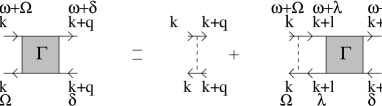
FIG. 7.: Bethe-Salpeter equation for $\Gamma$. Greek letters denote Matsubara frequencies.

FIG. 8.: Phases near the triple point. The solid line, $T_{1}$, separates the uniform and triangular phases, the short dashes, $T_{2}$, are the spinodal line and the long dashes, $T_{12}$, separate the triangular and unidirectional phase.

FIG. 9.: Phase diagram as in the previous figure. The dotted line is an extrapolation of $T_{12}$.

FIG. 10.: ${\tilde{u}}_{{\rm H}}(p)$ and $-{\tilde{u}}_{{\rm F}}(p)$. The unit of $p$ is the inverse magnetic length; the unit of energy is arbitrary.

FIG. 11.: Two near degenerate states $|A\rangle,|B\rangle$ with nonvanishing matrix element $\langle A|V_{{\rm HC}}|B\rangle$.

FIG. 12.: Diagram with two crossed interaction lines

FIG. 13.: Closed fermion loop.