Memory function approach to the Hall constant in strongly correlated electron systems

Abstract

The anomalous properties of the Hall constant in the normal state of high-$T_{c}$ superconductors are investigated within the single-band Hubbard model. We argue that the Mori theory is the appropriate formalism to address the Hall constant, since it aims directly at resistivities rather than conductivities. More specifically, the frequency dependent Hall constant decomposes into its infinite frequency limit and a memory function contribution. As a first step, both terms are calculated perturbatively in $U$ and on an infinite dimensional lattice, where $U$ is the correlation strength. If we allow $U$ to be of the order of twice the bare band width, the memory function contribution causes the Hall constant to change sign as a function of doping and to decrease as a function of temperature.

PACS numbers:

I Introduction

Since the discovery of high-$T_{c}$ superconductors ten years ago, the anomalous properties of their normal state have been the subject of intensive theoretical work. It is widely believed that a model of strongly correlated electrons already captures the basic ingredients of the relevant physics. In these models, the correlations are represented by a strong local interaction $U$. However, a coherent description of all anomalous properties on the basis of such a model is still lacking. The main problem is that exact calculations are generally feasible only in a small parameter regime and that most approximation schemes fail in capturing all aspects which are supposed to be important.

The Hall constant is especially hard to describe. One reason for this is that the Hall conductivity contains a three-point correlation function after it has been expanded to first order in the magnetic field. Then, the calculation of vertex corrections is a tough problem which, to our knowledge, has been attempted only in the case of a Fermi liquid and to leading order in the quasiparticle damping [1]. Moreover, since the frequency dependent Hall constant is given as a quotient of conductivities, the limit $\omega\rightarrow 0$ may be precarious due to resonances like the Drude peak. A more technical peculiarity of the Hall effect is due to the fact that the magnetic field is introduced via a vector potential which, formally, breaks the symmetry with respect to lattice translations. But even in the simplest case of a Bloch-Boltzmann description, the temperature dependence of the Hall constant may be difficult to reproduce, because the relaxation time cancels once it is assumed to be independent of momentum.

The measurements of the Hall constant in high-$T_{c}$ materials [2] reveal two major anomalous dependences: on temperature and on doping. Both cannot be understood within conventional band theory. For noninteracting tight-binding electrons on a two-dimensional square lattice, the Hall constant changes sign at half filling as the Fermi surface changes its shape from electronlike to holelike. In contrast, the Hubbard model in the large-$U$ limit exhibits an additional sign change below half filling which is purely due to correlations [3, 4]. In addition, in the limit $\delta\rightarrow 0$, i.e. near half filling, the Hall constant diverges according to a $1/\delta$ law [3, 4]. These properties are supposed to account for the doping dependence observed in, e.g., La_2-xSr_xCuO₄ [5, 6]. As for the anomalous temperature dependence of the Hall constant, the most striking features are: firstly, a strong decrease which is, in some cases, as fast as $1/T$ [2]; secondly, the lack of saturation above a fraction of the Debye temperature, typically $\sim 0.2-0.4T_{D}$ [7, 8], in contrast to what is expected in a Fermi liquid description with weak electron-phonon coupling [9]; and thirdly, a quadratic dependence of the Hall angle on temperature for not too large dopings [8, 10, 11]. In a Fermi liquid, the temperature dependence arises from an anisotropic relaxation time [7, 9]. If we assume scattering off phonons to be the main inelastic process, a temperature dependence is conceivable only below a certain temperature scale: Then, a sufficiently anisotropic Fermi surface causes the scattering to be confined to those regions of the Fermi surface, where small momentum transfers are possible. For high enough temperatures, this kinematic restriction is lifted and the scattering becomes isotropic, thus leading to a cancellation of the relaxation time. The cross-over temperature is given by $\sim 0.2-0.4T_{D}$. The universally observed decrease of the Hall constant as a function of temperature in almost all high-$T_{c}$ compounds up to temperatures clearly beyond this temperature scale must therefore be due to electronic correlations as well.

In the following, we investigate the Hall effect on the basis of the simplest model of strongly correlated electrons, namely the single-band Hubbard model on a hypercubic lattice in $d$ dimensions with nearest-neighbour hopping. This model, along with Mori’s formalism used to represent the Hall constant, is introduced in Sec. II. In this theory, the Hall constant is given as the sum of its infinite frequency limit ($R_{H}^{\infty}$) and a memory function contribution. The former term was first considered by Shastry, Shraiman and Singh [3]. Our emphasis is on the memory function term which represents the deviation of the Hall constant from $R_{H}^{\infty}$ for finite frequencies and thus cannot be neglected when considering the case of zero frequency. The advantage of our representation of the Hall constant is that we do not have to cope with a quotient of conductivities as opposed to the usual approaches. This is why the Hall constant at low frequencies becomes less sensitive to the detailed resonance structure of the conductivities. In the remainder of this paper, this advantage is exploited for the range of weak to intermediate correlation strengths, while the opposite limit of strong correlations will be addressed in a forthcoming paper [12]. In Sec. III, we proceed by calculating the memory function to second order in the Hubbard interaction and to first order in the magnetic field. Expansion with respect to the magnetic field leads to a decomposition of the memory function into two terms, namely a two-point and a three-point correlation function. Both contributions are evaluated exactly in infinite spatial dimensions. Our results indicate that the memory function term is important. Only then, a precursor effect of the sign change of the Hall constant as a function of doping appears even in perturbation theory. Moreover, when extrapolating our results to $U$ values of the order of twice the free band width $W$, we get most of the qualitative features observed in, e.g., La_2-xSr_xCuO₄: the sign change with respect to doping and the decrease of the Hall constant up to unusually high temperatures, characteristic of most high-$T_{c}$ compounds. Finally, in Sec. IV, we summarize our main results.

II Theoretical framework

A Single-band Hubbard model

The single-band Hubbard model on a d-dimensional hypercubic lattice in a magnetic field reads

$$\hat{H} = \hat{T}+\hat{V}\,,$$ (1)

$$\hat{T} = -t\sum_{<ij>}P_{ij}c_{i\sigma}^{+}c_{j\sigma}\,,$$ (2)

$$\hat{V} = U\sum_{i}\hat{n}_{i\uparrow}\hat{n}_{i\downarrow}\,,$$ (3)

where the sum in the hopping term $\hat{T}$ is restricted to nearest neighbours and $\hat{V}$ is the Hubbard repulsion. The Peierls phase factor $P_{ij}=\exp(ie\int_{j}^{i}\,\vec{A}(t,\vec{r}\,)\;d\vec{r}\,)$ guarantees the gauge invariance [13] and the sign of the charge $e$ is chosen to be negative. Since only nearest neighbour hops are taken into account, we may approximate

$$P_{ij}\simeq e^{ie\vec{A}(\vec{R}_{j})(\vec{R}_{i}-\vec{R}_{j})}\;,$$ (4)

where $R_{i}$ denotes the lattice vector to site $i$. The vector potential decomposes into two terms describing the electric and magnetic field, respectively:

$$\vec{A}(t,\vec{r}\,) = \vec{A}^{el}(t)+\vec{A}^{mag}(\vec{r}\,)\,,$$ (5)

$$\vec{E}(t) = -\frac{\partial}{\partial t}\vec{A}^{el}(t)\,,$$ (6)

$$\vec{H} = rot\,\vec{A}^{mag}(\vec{r}\,)\,.$$ (7)

In linear response theory with respect to the electric field, the latter appears only in the definition of the current operator. More precisely, the current operator is defined as the following functional derivative:

$$\hat{J}_{\nu}:=-\frac{1}{e}\frac{\delta\hat{H}(t)}{\delta A_{\nu}^{el}(t)}\Bigg{|}_{A^{el}=0\,.}$$ (8)

The homogeneous magnetic field is chosen to point in the $z$-direction and it is advantageous to fix the gauge from the very beginning according to the Landau choice

$$\vec{A}^{mag}(\vec{R})=R_{x}H\hat{y}\,,$$ (9)

since then, translational symmetry is broken only in one dimension, namely the $x$-direction. $\hat{y}$ is a primitive lattice vector. We need the current operator only up to first order in the magnetic field:

$$\hat{J}_{\nu} = \hat{J}_{\nu}^{(0)}+\delta\hat{J}_{\nu}\,,$$ (10)

$$\hat{J}_{\nu}^{(0)} = it\sum_{\vec{R},\vec{R}+\vec{\delta},\sigma}\,\delta_{\nu}\,c_{\sigma}^{+}(\vec{R}+\vec{\delta})c_{\sigma}(\vec{R}),$$ (11)

$$\delta\hat{J}_{\nu} = -et\sum_{\vec{R},\vec{R}+\vec{\delta},\sigma}\,\delta_{\nu}\,\vec{\delta}\vec{A}^{mag}(\vec{R})c_{\sigma}^{+}(\vec{R}+\vec{\delta})c_{\sigma}(\vec{R})\;.$$ (12)

Here, $\vec{\delta}$ is a nearest neighbour vector and the summation is over pairs of nearest neighbours. Note, however, that due to the gauge fixation (9), we cannot choose periodic boundary conditions in the $x$-direction. Thus, if $\vec{\delta}$ points in the $x$-direction, we have to carry out the sums in such a way that the components $R_{x}$ and $R_{x}+\delta_{x}$ are simultaneously elements of the set consisting of the $x$-coordinates of all lattice sites, e.g. $\{R_{x}^{min},R_{x}^{min}+1,\ldots,R_{x}^{max}\}$. Here, it is assumed that the lattice has $N_{x}$ sites in the $x$-direction which implies $R_{x}^{max}\equiv R_{x}^{min}+N_{x}-1$. Of course, observable quantities are not allowed to depend on the lattice location $R_{x}^{min}$. The hopping term is expanded analogously, yielding:

$$\hat{T} = \hat{T}^{(0)}+\delta\hat{T}\,,$$ (13)

$$\hat{T}^{(0)} = -t\sum_{\vec{R},\vec{R}+\vec{\delta},\sigma}\,c_{\sigma}^{+}(\vec{R}+\vec{\delta})c_{\sigma}(\vec{R}),$$ (14)

$$\delta\hat{T} = -iet\sum_{\vec{R},\vec{R}+\vec{\delta},\sigma}\,\vec{\delta}\vec{A}^{mag}(\vec{R})c_{\sigma}^{+}(\vec{R}+\vec{\delta})c_{\sigma}(\vec{R})\;.$$ (15)

The term without magnetic field, i.e. Eq. (14), becomes diagonal in crystal momentum space with a band dispersion $\epsilon_{\vec{k}}=-2t\sum_{j=1}^{d}\cos k_{j}$.

B Mori theory

In this subsection, the basics of Mori’s memory function formalism is reviewed briefly. For further details, see e.g. Ref. [14]. The best known application of Mori theory is the description of many particle systems in the hydrodynamic regime [15]. There, one is only interested in the dynamics of the hydrodynamic variables. They are characterized by the fact that their transport is restricted by conservation laws or by broken symmetries. Thus, they are bound to vary on a time scale that is very slow in comparison to that of all the other degrees of freedom. Now, the Mori theory enables one to separate these two time scales: The equations of motion of the hydrodynamic variables take on the form of coupled integro-differential equations. The corresponding integral kernels of these so called Mori equations are memory functions in which the influence of all the other degrees of freedom is accumulated, hence the name “memory function”. In this context of hydrodynamics, the memory functions are rapidly varying functions, whose effect may be simulated by damping constants. Then, the Mori equations take on a form analogous to that of the Langevin equation for a particle undergoing Brownian motion. However, the validity of the Mori equations is not restricted to the special set of hydrodynamic variables. In the simplest case, one sets up the Mori theory for those observables that constitute the correlation functions one is interested in. This leads to representations for the unknown correlation functions in terms of memory functions in which all analytic properties are fulfilled by construction. On the other hand, it may be difficult to find an approximate expression for a given memory function.

1 basic notions

The Liouville space ${\cal L}$ is defined as the linear vector space over the field of complex numbers whose elements are the linear operators in the familiar Hilbert space of quantum mechanics, and where the usual operations like scalar multiplication etc. hold. In this Liouville space exist linear operators that are called superoperators to distinguish them from the usual ones. (Henceforth, normal operators are denoted with a hat, superoperators not.) The most important superoperator is the Liouville operator $L$, which maps a given operator onto its commutator with the Hamiltonian:

$$L\hat{A}=[\hat{H},\hat{A}]\,.$$ (16)

An other important class of superoperators are superprojectors. However, their definition implies a scalar product in ${\cal L}$. In the context of response functions, the most convenient scalar product turns out to be the so called Mori product

$$(\hat{A}|\hat{B}):=\frac{1}{\beta}\int_{0}^{\beta}\,d\tau\,<\;e^{\tau L}\hat{A}^{+}\cdot\hat{B}\;>\;,$$ (17)

where $<\ldots>$ denotes the thermal average and $\beta$ is the inverse temperature. On the basis of this scalar product, we may now speak of adjoint superoperators $S$ and $S^{+}$, and thus of unitary and Hermitian ones in the usual sense. The projector $P$ that projects onto the subspace of ${\cal L}$ spanned by linearly independent elements $|\hat{G}_{i})$, reads:

$$P=\sum_{ij}|\hat{G}_{i})g_{ij}(\hat{G}_{j}|,$$ (18)

where the metric $g_{ij}$ is the inverse of the matrix $(\hat{G}_{i}|\hat{G}_{j})$, i.e. $\sum_{k}\,g_{ik}(\hat{G}_{k}|\hat{G}_{j})=\delta_{ij}$. In fact, this implies the idempotence property $P^{2}=P$. Finally, the definition of the Mori product implies the validity of the so called Kubo identity

$$\beta(\hat{A}|L|\hat{B})=<[\hat{A}^{+},\hat{B}]>\;,$$ (19)

which will play an important role.

2 Memory function approach to the Hall constant

From Eq. (19) follows a representation for the current-current correlation function $\ll\hat{J}_{\nu}\,;\,\hat{J}_{\mu}\gg_{z}$ , defined as the Laplace transform of $-i<[e^{iLt}\hat{J}_{\nu}\,,\,\hat{J}_{\mu}]>$:

$$\ll\hat{J}_{\nu}\,;\,\hat{J}_{\mu}\gg_{z}=-\beta(\hat{J}_{\mu}|\frac{L}{z+L}|\hat{J}_{\nu})\equiv-\chi_{\mu\nu}(z)\,.$$ (20)

Here, $z$ is a complex frequency, which ultimately has to be specialized to $\omega+i0^{+}$. For formal manipulations, however, it is more convenient to deal with the complex frequency $z$ rather than with $\omega$. The last expression has to be inserted into the Kubo formula for the conductivity tensor,

$$\sigma_{\nu\mu}(z)=\frac{ie^{2}}{Nz}\{<\hat{\tau}_{\nu\mu}>+\ll\hat{J}_{\nu}\,;\,\hat{J}_{\mu}\gg_{z}\}\,,$$ (21)

where $<\hat{\tau}_{\nu\mu}>$ arises from the equilibrium part of the current and is defined as the second functional derivative of the Hamiltonian with respect to the external electric field:

$$\hat{\tau}_{\nu\mu}:=\frac{1}{e^{2}}\frac{\delta^{2}\hat{H}(t)}{\delta A_{\nu}^{el}(t)\,\delta A_{\mu}^{el}(t)}\Bigg{|}_{A^{el}=0\;.}$$ (22)

In the Hubbard model (1), its expectation value is given as $<\hat{\tau}_{\nu\mu}>=2t\sum_{\vec{k}\sigma}cos\,k_{x}<\hat{n}_{\vec{k}\sigma}>$, i.e. as the average kinetic energy per dimension. Using the fact $\lim_{z\rightarrow 0}z\,\sigma_{\nu\mu}(z)=0$ which holds for a metal in the normal state, we show that $<\hat{\tau}_{\nu\mu}>$ also equals the static susceptibility $\chi^{0}$, defined through $\chi_{\mu\nu}(z=0)\equiv\delta_{\mu\nu}\,\chi^{0}\,$:

$$\chi^{0}=\beta(\hat{J}_{x}|\hat{J}_{x})=<\hat{\tau}_{xx}>=-\frac{1}{d}<\hat{T}>\;.$$ (23)

Thus, the conductivity tensor may be written as

$$\sigma_{\nu\mu}(z)=\frac{e^{2}}{N}\beta(\hat{J}_{\mu}|\frac{i}{z+L}|\hat{J}_{\nu})\equiv\frac{e^{2}}{N}C_{\mu\nu}(z)\,.$$ (24)

In order to represent the relaxation functions $C_{\mu\nu}(z)$ in terms of memory functions, we introduce the superprojector $P$ that projects onto the subspace of ${\cal L}$ spanned by the current operators $\hat{J}_{x}$ and $\hat{J}_{y}$:

$$P=\frac{\beta}{\chi^{0}}\sum_{\nu=x,y}|\hat{J}_{\nu})(\hat{J}_{\nu}|\,,$$ (25)

and the complementary superprojector $Q=1-P$. By making use of the operator identity $\frac{1}{a+b}=\frac{1}{a}-\frac{1}{a}b\frac{1}{a+b}$ with $a\equiv z+LQ$ and $b\equiv LP$, we find:

$$C_{\mu\nu}(z) = \frac{i}{z}\chi^{0}\delta_{\mu\nu}-\frac{1}{z}R_{\mu\alpha}(z)C_{\alpha\nu}(z)\,,$$ (26)

$$R_{\mu\nu}(z) \equiv \frac{\beta}{\chi^{0}}(\hat{J}_{\mu}|\frac{z}{z+LQ}L|\hat{J}_{\nu})$$ (27)

$$\equiv \Omega_{\mu\nu}+iM_{\mu\nu}(z)\,.$$ (28)

The terms in the last equation are the frequency and the memory matrix, respectively:

$$\Omega_{\mu\nu} \equiv \frac{1}{\chi^{0}}<[\hat{J}_{\mu}\,,\,\hat{J}_{\nu}]>\;,$$ (29)

$$M_{\mu\nu}(z) \equiv \frac{\beta}{\chi^{0}}(QL\hat{J}_{\mu}|\frac{i}{z+QLQ}|QL\hat{J}_{\nu})\,.$$ (30)

The last equation shows that the dynamics of the memory functions is governed by $QLQ$ rather than $L$. Solving Eq. (26) for the matrix ${\bf C}(z)$ leads to

$${\bf C}(z)=i\chi^{0}\left(z{\bf 1}+{\bf\Omega}+i{\bf M}(z)\right)^{-1}\,.$$ (31)

Together with Eq. (24), this demonstrates that the Mori theory enables us to calculate directly the resistivity tensor. Therefore, the desired representation for the dynamical Hall constant can be read off from the last equation:

$$R_{H}(z)=\frac{N}{ie^{2}\chi^{0}}\lim_{H\rightarrow 0}\frac{\Omega_{xy}+iM_{xy}(z)}{H}\;.$$ (32)

Since the memory function term will be shown to vanish in the high frequency limit as $1/z^{2}$, the first term represents the high frequency limit of the Hall constant considered by Shastry et al. [3]:

$$R_{H}^{\infty}=\frac{N}{ie^{2}\chi^{0}}\lim_{H\rightarrow 0}\frac{\Omega_{xy}}{H}\;.$$ (33)

Moreover, $\Omega_{xy}$ is the generalization of the cyclotron frequency to the lattice case. Therefore, within a Boltzmann equation approach, only the term (33) is considered. The goal of the subsequent sections is to investigate the memory function term $M(z)\equiv M_{xy}(z)$ for finite frequencies.

3 Analytic properties

The analytic properties of $M(z)$ in Eq. (32) may all be derived on the basis of Eq. (30). An alternative procedure is to solve Eq. (31) for ${\bf M}(z)$ and go back to the analytic properties of the current susceptibilities $\chi_{\mu\nu}(z)$, cf. Eq. (20). $M(z)$ reads in terms of the susceptibilities $\chi_{\mu\nu}(z)$:

$$iM(z)=\frac{z\chi^{0}\chi_{xy}(z)}{(\chi^{0}-\chi_{xx}(z))^{2}}-\frac{<[\hat{J}_{x}\,,\,\hat{J}_{y}]>}{\chi^{0}}\;.$$ (34)

From time reversal invariance, homogenity of time and the fact that the current operators are Hermitian, we may deduce the following symmetry properties [15]:

$$\chi_{xx}(-z) = \chi_{xx}(z)\,,$$ (35)

$$\chi_{xx}^{*}(z) = \chi_{xx}(z^{*})\,,$$ (36)

$$\chi_{xy}(-z) = -\chi_{xy}(z)\,,$$ (37)

$$\chi_{xy}^{*}(z) = -\chi_{xy}(z^{*})\,.$$ (38)

Together with Eq. (34), this implies:

$$M(-z) = M(z)\,,$$ (39)

$$M^{*}(z) = M(z^{*})\,.$$ (40)

$M(z)$ can be represented as a spectral integral

$$M(z)=\int\frac{d\omega}{\pi}\,\frac{M^{\prime\prime}(\omega)}{\omega-z}\,,$$ (41)

where the spectral function $M^{\prime\prime}(\omega)$ is given by the discontinuity across the real axis:

$$M(\omega\pm i0^{+})=M^{\prime}(\omega)\pm iM^{\prime\prime}(\omega)\,.$$ (42)

From the analytic properties (40), it follows that $M^{\prime}(\omega)$ and $M^{\prime\prime}(\omega)$ are real functions satisfying

$$M^{\prime}(-\omega) = M^{\prime}(\omega)\,,$$ (43)

$$M^{\prime\prime}(-\omega) = -M^{\prime\prime}(\omega)\,.$$ (44)

Thus, two further conclusions can be drawn: Firstly, only even powers in $1/z$ contribute to the high frequency expansion of $M(z)$. And secondly, the quotient $M^{\prime\prime}(\omega)/\omega$ must be integrable around $\omega=0$,

$$\int_{-\infty}^{\infty}d\omega\,M^{\prime\prime}(\omega)/\omega<\infty,$$ (45)

which can be seen from the fact that the dc-Hall constant contains this integral. Note, that we need not understand this expression as a Principal value integral due to the fact that the integrand is even.

III Perturbation theory

Despite many interesting works on the normal state Hall effect of high-$T_{c}$ superconductors, a calculation that incorporates all the complicated many-body correlations exactly within a microscopic model is still lacking. The following treatment of the Hall constant closes this gap at least in the perturbation-theoretical regime. On the other hand, the relevant parameter regime is believed to be the strong correlation limit rather than the weak one. However, it turns out that the final expression may well describe the observed dependencies on temperature and on doping at least qualitatively, if we allow $U$ to be extrapolated to values of the order of the free band width $W$. Thus, a precursor effect of the anomalous dependences clearly shows up even in the regime of weak correlations.

A Approximation

The perturbation-theoretical treatment of the Hall constant is by no means straightforward. As is well known, the evaluation of response functions like $\chi_{\mu\nu}(z)$ of Eq. (20) by expansion in a small interaction parameter fails because, as an artefact of such an expansion, these functions become singular for small frequencies $z$. This difficulty was resolved by Götze and Wölfle [16] some time ago by means of a memory function approach. They calculated the memory function perturbatively, which, at first, is valid only at high enough frequencies. It turns out, however, that their expression for the memory function depends only smoothly on frequency below a certain frequency scale and tends to a constant in the limit $\omega\rightarrow 0$. Furthermore, in their approximation scheme the correct resonance structure of the studied response functions is inherently built in. Thus, their results could be used in the whole frequency regime including the hydrodynamic one. However, we cannot carry over their analysis straightforwardly to the present problem, because otherwise, we would encounter a spurious singularity in the limit that is of most interest, i.e. $\omega\rightarrow 0$.

In this subsection, we identify the precondition which is necessary to obtain regular expressions in this limit and that was fulfilled trivially in the applications of Ref. [16] but is not in our case. Since this condition does not affect the correct description of the local interaction $U$, we may take it as an approximation. By using Mori’s formalism, we shall see that once this condition is assumed to be satisfied no further approximations have to be made. This last point cannot be seen in the more intuitive introduction of the memory function concept as given in Ref. [16] and shows that the extrapolation to low frequencies therein is exact.

Perturbation theory is based on the following decomposition of the Liouville operator:

$$L=L_{0}+L_{1}\,,$$ (46)

where $L_{0}$ and $L_{1}$ are assigned to the hopping and interaction term of the Hubbard hamiltonian (1), respectively. The perturbation-theoretical regime is given by the condition $U\ll W$, where $W$ is the width of the free band and thus represents the characteristic energy scale introduced by $L_{0}$. The precondition to obtain a regular expression for the memory function $M(z)$ for all frequencies to leading order in $U$ is that the relevant operators $\hat{J}_{x}$ and $\hat{J}_{y}$ span a subspace of ${\cal L}$ that is invariant with respect to actions of $L_{0}$ [14]. If this condition were satisfied in our case, it would take on the form

$$L_{0}\hat{J}_{\nu}=[\hat{T},\hat{J}_{\nu}]=\hat{J}_{\mu}^{(0)}\;\Omega_{\mu\nu}^{0}\,,$$ (47)

where $\nu,\mu=x,y$ and summation over repeated indices is implied. This can be checked by inserting these equations into $(\hat{J}_{\lambda}|\ldots)_{0}$ and comparing the result with the definition (29). $(\ldots|\ldots)_{0}$ is the Mori product with respect to $L_{0}$. Henceforth, bracketed indices refer to the magnetic field and unbracketed ones to the decomposition (46). Unfortunately, the conditions (47) are not satisfied in the Hubbard model. Instead, we derive with the help of Eqs. (10)-(12) and (13)-(15) (see the appendix):

$$[\hat{T},\hat{J}_{x}]\,=\frac{\sum_{\vec{k}\sigma}\,\cos k_{x}\,\sin k_{y}\,\hat{n}_{\vec{k}\sigma}}{\sum_{\vec{k}\sigma}\,\cos k_{x}\,\cos k_{y}\,n_{\vec{k}\sigma}^{0}}\;<[\hat{J}_{y},\hat{J}_{x}]>_{0}\;,$$ (48)

which should be equal to

$$\frac{\sum_{\vec{k}\sigma}\,\sin k_{y}\,\hat{n}_{\vec{k}\sigma}}{\sum_{\vec{k}\sigma}\,\cos k_{y}\,n_{\vec{k}\sigma}^{0}}\;<[\hat{J}_{y},\hat{J}_{x}]>_{0}=\hat{J}_{y}^{(0)}\Omega_{yx}^{0}\;.$$ (49)

This is obviously not the case. Similarly, we find

$$[\hat{T},\hat{J}_{y}]\,=\frac{\sum_{\vec{k}\sigma}\,\sin k_{x}\,\cos k_{y}\,\hat{n}_{\vec{k}\sigma}}{\sum_{\vec{k}\sigma}\,\cos k_{x}\,\cos k_{y}\,n_{\vec{k}\sigma}^{0}}\;<[\hat{J}_{x},\hat{J}_{y}]>_{0}\;,$$ (50)

instead of

$$\frac{\sum_{\vec{k}\sigma}\,\sin k_{x}\,\hat{n}_{\vec{k}\sigma}}{\sum_{\vec{k}\sigma}\,\cos k_{x}\,n_{\vec{k}\sigma}^{0}}\;<[\hat{J}_{x},\hat{J}_{y}]>_{0}=\hat{J}_{x}^{(0)}\Omega_{xy}^{0}\;.$$ (51)

However, the conditions (47) become exact in the continuum limit or in the limit of small band fillings. This is seen if we take explicitly into account the lattice spacing $a$ in the arguments of the trigonometric functions which we tacitly have set equal to 1. Then we may expand $\cos k_{\nu}a\simeq 1$ and $\sin k_{\nu}a\simeq k_{\nu}a$ which proves the statement immediately. Thus, the violation of the conditions (47) on the lattice reflects its reduced symmetry in comparison with free space. Since the conditions (47) are properties of the free model, we may assume their approximate validity without taking the risk of not describing the local interactions (3) correctly.

Before proceeding, we show how the conditions (47) appear within the formalism outlined in Ref. [16]. We expand Eq. (34) in the frequency regime, where the expression $|\chi_{xx}(z)/\chi^{0}|$ is very small, i.e. for high enough frequencies and use a couple of times equations of motion for correlation functions $\ll\hat{A};\hat{B}\gg_{z}$. Thus we may show that $M(z)$ can be represented as follows (cf. Eq. (57):

$$i\chi^{0}M(z)\simeq-\frac{\ll\hat{K}_{x};\hat{K}_{y}\gg_{z}^{0}}{z}+R(z)\,.$$ (52)

The first term will be investigated in the next subsection and turns out to be regular for all frequencies; $R(z)$ can be written as:

$$R(z) = \ll\hat{J}_{x};[\hat{T},\hat{J}_{y}]\gg_{z}-\ll[\hat{T},\hat{J}_{x}];\hat{J}_{y}\gg_{z}+2\Omega^{0}_{xy}\chi_{xx}(z)$$ (53)

$$= \frac{2<[\hat{J}_{x},\hat{J}_{y}]>_{0}}{\chi^{0}}\frac{\phi_{xx}(z)-\phi_{xx}(0)}{z^{2}}\;,$$ (54)

where $\phi_{xx}(z)\equiv\ll\hat{K}_{x};\hat{K}_{x}\gg_{z}^{0}$. Calculating the function $\phi_{xx}(z)$ following the lines outlined in the next subsection, we may prove that $R(z)$ is indeed divergent in the limit $z\rightarrow 0$, which, however, is an artefact of perturbation theory. The first representation of $R(z)$ in the last set of equations shows that the condition (47) implies $R(z)$ to vanish identically, if we take into account the symmetry properties $\Omega_{xy}^{0}=-\Omega_{yx}^{0}$ and $\chi_{xx}(z)=\chi_{yy}(z)$.

B Reduction to ordinary correlation functions

We are interested in the memory function appearing in Eq. (32), whose Laplace transform is given according to Eq. (30) as

$$M(t)=\frac{\beta}{\chi^{0}}(QL\hat{J}_{x}|e^{iQLQt}|QL\hat{J}_{y})\,.$$ (55)

Due to the approximation (47), the free part $L_{0}$ of the Liouville operator does not contribute to the operator $QL|\hat{J}_{\nu})$. Hence, to leading order in the interaction strength $U$, we obtain

$$M(t)=\frac{\beta}{\chi^{0}}(Q_{0}L_{1}\hat{J}_{x}|e^{iQ_{0}L_{0}Q_{0}t}|Q_{0}L_{1}\hat{J}_{y})_{0\,.}$$ (56)

Since $Q_{0}$ commutes with $L_{0}$ and because of the idempotence of $Q_{0}$ [14], we may free ourselves of all superprojectors $Q_{0}$ with the exception of one, say, that within the “ket” $|Q_{0}L_{1}\hat{J}_{y})$. However, even this last appearance of $Q_{0}$ may be omitted, since its part $P_{0}$ leads to a term proportional to the following first order expression of the frequency matrix [14]: $\Omega_{\nu\mu}^{1}=g^{0}_{\nu\lambda}(\hat{J}_{\lambda}|L_{1}|\hat{J}_{\mu})_{0}$. Here summation over equal indices is implied. However, the frequency matrix is easily traced back to $n_{\vec{k}\sigma}=<c_{\vec{k}\sigma}^{+}c_{\vec{k}\sigma}>$, whose first order contribution vanishes. Thus, $\Omega_{\nu\mu}^{1}$ vanishes as stated and we arrive at $M(z)=(\beta/\chi^{0})(\hat{K}_{x}|i/(z+L_{0})|\hat{K}_{y})_{0}$, where we have defined

$$\hat{K}_{\nu}\equiv[\hat{V},\hat{J}_{\nu}]\,.$$ (57)

With the identity $z/(z+L_{0})=1-L_{0}/(z+L_{0})$ and the symmetry property $\ll\hat{K}_{x};\hat{K}_{y}\gg_{-z}^{0}=-\ll\hat{K}_{x};\hat{K}_{y}\gg_{z}^{0}$, which may be traced back to Eq. (37) by means of two equations of motion, we eventually arrive at

$$i\chi^{0}M(z)=\,-\;\frac{\ll\hat{K}_{x};\hat{K}_{y}\gg_{z}^{0}}{z}\;.$$ (58)

Now, we must evaluate this correlation function for the free tight binding model (13) to leading first order in the magnetic field. In order to derive explicit expressions for the operators (57), we introduce the following combination of Blochoperators:

$$\hat{A}^{\sigma}_{\vec{k}_{1},\vec{k}_{2}|\vec{k}|\vec{q}}\equiv c_{\vec{k}_{1}\sigma}^{+}c_{\vec{k}_{2}\sigma}c_{\vec{k}-\vec{q}|-\sigma}^{+}c_{\vec{k}|-\sigma}\;.$$ (59)

This is the basic building block for the operators $\hat{K}_{\nu}$. To see this, we insert Eqs. (3) and (10)-(12) into the definition (57) and write the result in terms of Blochoperators. We find:

$$\hat{K}_{\nu} = \hat{K}_{\nu}^{0}+\delta\hat{K}_{\nu}\,,$$ (60)

$$\hat{K}_{\nu}^{(0)} = -\frac{U}{N}\sum_{\vec{k}_{1}\vec{k}_{2}\vec{k}\vec{q}\sigma}\;\left[B_{\nu}(\vec{k}_{1},\vec{k}_{2}+\vec{q}\,)-B_{\nu}(\vec{k}_{1}-\vec{q},\vec{k}_{2})\right]\hat{A}^{\sigma}_{\vec{k}_{1},\vec{k}_{2}|\vec{k}|\vec{q}\;,}$$ (61)

$$\delta\hat{K}_{x} = 0\;,$$ (62)

$$\delta\hat{K}_{y} = Het\frac{U}{N}\sum_{\vec{k}_{1}\vec{k}_{2}\vec{k}\vec{q}\sigma}\;\left[C(\vec{k}_{1},\vec{k}_{2}+\vec{q}\,)-C(\vec{k}_{1}-\vec{q},\vec{k}_{2})\right]\hat{A}^{\sigma}_{\vec{k}_{1},\vec{k}_{2}|\vec{k}|\vec{q}\;,}$$ (63)

where the matrices $B_{\nu}(\vec{k}_{1},\vec{k}_{2})$ and $C(\vec{k}_{1},\vec{k}_{2})$ are defined in the appendix, cf. Eqs. (A2) and (A3). Since $\delta\hat{K}_{x}$ vanishes, the expansion of the correlation function of Eq. (58) to first order in the magnetic field reads:

$$\ll\hat{K}_{x};\hat{K}_{y}\gg_{z}^{0} = C^{II}(z)+C^{III}(z)\,,$$ (64)

$$C^{II}(z) = \ll\hat{K}_{x}^{(0)};\delta\hat{K}_{y}\gg^{0(0)}_{z}\,\,\,,$$ (65)

$$C^{III}(z) = \ll\hat{K}_{x}^{(0)};\hat{K}_{y}^{(0)}\gg^{0(1)}_{z}\,\,\,.$$ (66)

Obviously, it is sufficient to calculate the correlation function consisting of operators (59) within the tight binding model (13), however, to first order in the magnetic field. But first, we note that the functions (65) and (66) are two- and three-point correlation functions, respectively. This is explicitly seen within the Matsubara representation where the expansion of $\ll\hat{K}_{x};\hat{K}_{y}\gg_{z}^{0}$ up to first order in the “perturbation” (15) yields:

$$C^{II}(i\omega_{m}) = -\frac{1}{\beta}\int_{0}^{\beta}\int_{0}^{\beta}d\tau\,d\tau^{\prime}\,<T_{\tau}\left\{\hat{K}_{x}^{(0)}(\tau)\,\delta\hat{K}_{y}(\tau^{\prime})\right\}>_{0}^{(0)}\;e^{i\omega_{m}(\tau-\tau^{\prime})}\;,$$ (67)

$$C^{III}(i\omega_{m}) = \frac{1}{\beta}\int_{0}^{\beta}\int_{0}^{\beta}\int_{0}^{\beta}d\tau\,d\tau^{\prime}\,d\tau^{\prime\prime}\,<T_{\tau}\left\{\hat{K}_{x}^{(0)}(\tau)\,\hat{K}_{y}^{(0)}(\tau^{\prime})\delta\hat{T}(\tau^{\prime\prime})\right\}>_{0}^{(0)}\;e^{i\omega_{m}(\tau-\tau^{\prime})}\,.$$ (68)

C Expansion to first order in the magnetic field

As already mentioned, our next goal is to calculate the correlation function generated by the operators (59) up to first order in the magnetic field. This is accomplished by means of its equation of motion with respect to the tight binding hamiltonian (13):

$$(z+\epsilon_{\vec{k}-\vec{q}}-\epsilon_{\vec{k}} + \epsilon_{\vec{k}_{1}}-\epsilon_{\vec{k}_{2}})\ll\hat{A}^{\sigma}_{\vec{k}_{1},\vec{k}_{2}|\vec{k}|\vec{q}}\;;\;\hat{A}^{\sigma^{\prime}}_{\vec{k}^{\prime}_{1},\vec{k}^{\prime}_{2}|\vec{k}^{\prime}|\vec{q^{\prime}}}\gg_{z}$$ (69)

$$= <[\hat{A}^{\sigma}_{\vec{k}_{1},\vec{k}_{2}|\vec{k}|\vec{q}}\;,\;\hat{A}^{\sigma^{\prime}}_{\vec{k}^{\prime}_{1},\vec{k}^{\prime}_{2}|\vec{k}^{\prime}|\vec{q^{\prime}}}]>-\ll[\,\delta\hat{T}\,,\;\hat{A}^{\sigma}_{\vec{k}_{1},\vec{k}_{2}|\vec{k}|\vec{q}}\;]\;;\;\hat{A}^{\sigma^{\prime}}_{\vec{k}^{\prime}_{1},\vec{k}^{\prime}_{2}|\vec{k}^{\prime}|\vec{q^{\prime}}}\gg_{z}^{(0)}\,\,\,.$$ (70)

Here and in the following, the index $0$ is omitted. The expansion of the expectation value on the Rhs. with respect to the magnetic field is standard [17] and yields:

$$<[\hat{A}^{\sigma}_{\vec{k}_{1},\vec{k}_{2}|\vec{k}|\vec{q}} \hat{A}^{\sigma^{\prime}}_{\vec{k}^{\prime}_{1},\vec{k}^{\prime}_{2}|\vec{k}^{\prime}|\vec{q^{\prime}}}]>$$ , (71)

$$= <[\hat{A}^{\sigma}_{\vec{k}_{1},\vec{k}_{2}|\vec{k}|\vec{q}}\;,\;\hat{A}^{\sigma^{\prime}}_{\vec{k}^{\prime}_{1},\vec{k}^{\prime}_{2}|\vec{k}^{\prime}|\vec{q^{\prime}}}]>^{(0)}-<\hat{v}\;[\hat{A}^{\sigma}_{\vec{k}_{1},\vec{k}_{2}|\vec{k}|\vec{q}}\;,\;\hat{A}^{\sigma^{\prime}}_{\vec{k}^{\prime}_{1},\vec{k}^{\prime}_{2}|\vec{k}^{\prime}|\vec{q^{\prime}}}]>^{(0)}\,\,,$$ (72)

where $\hat{v}$ arises from the expansion of the $S$-matrix related to the “perturbation” (15) and is therefore given by

$$\hat{v}=\int_{0}^{\beta}d\tau\;e^{\tau(\hat{T}^{(0)}-\mu\hat{N})}\;\delta\hat{T}\;e^{-\tau(\hat{T}^{(0)}-\mu\hat{N})}\,\,.$$ (73)

With the representation of $\delta\hat{T}$ in terms of Blochoperators,

$$\delta\hat{T}=-ietH\sum_{\vec{k}_{1}\vec{k}_{2}\sigma}D(\vec{k}_{1},\vec{k}_{2})c_{\vec{k}_{1}\sigma}^{+}c_{\vec{k}_{2}\sigma\;,}$$ (74)

where the matrix $D(\vec{k}_{1},\vec{k}_{2})$ is also defined and further evaluated in the appendix (cf. Eq. (A4)), we find more explicitly:

$$\hat{v}=-ietH\sum_{\vec{k}_{1}\vec{k}_{2}\sigma}D(\vec{k}_{1},\vec{k}_{2})\frac{e^{\beta(\epsilon_{\vec{k}_{1}}-\epsilon_{\vec{k}_{2}})}-1}{\epsilon_{\vec{k}_{1}}-\epsilon_{\vec{k}_{2}}}c_{\vec{k}_{1}\sigma}^{+}c_{\vec{k}_{2}\sigma\;.}$$ (75)

Inserting the expansion (72) into Eq. (70), we obtain the following zeroth and first order terms for the correlation function to be determined:

$$\ll\hat{A}^{\sigma}_{\vec{k}_{1},\vec{k}_{2}|\vec{k}|\vec{q}}\;;\;\hat{A}^{\sigma^{\prime}}_{\vec{k}^{\prime}_{1},\vec{k}^{\prime}_{2}|\vec{k}^{\prime}|\vec{q^{\prime}}}\gg_{z}^{(0)} = \frac{<[\hat{A}^{\sigma}_{\vec{k}_{1},\vec{k}_{2}|\vec{k}|\vec{q}}\;,\;\hat{A}^{\sigma^{\prime}}_{\vec{k}^{\prime}_{1},\vec{k}^{\prime}_{2}|\vec{k}^{\prime}|\vec{q^{\prime}}}]>^{(0)}}{z+\epsilon_{\vec{k}-\vec{q}}-\epsilon_{\vec{k}}+\epsilon_{\vec{k}_{1}}-\epsilon_{\vec{k}_{2}}}\;\;,$$ (76)

$$\ll\hat{A}^{\sigma}_{\vec{k}_{1},\vec{k}_{2}|\vec{k}|\vec{q}}\;;\;\hat{A}^{\sigma^{\prime}}_{\vec{k}^{\prime}_{1},\vec{k}^{\prime}_{2}|\vec{k}^{\prime}|\vec{q^{\prime}}}\gg_{z}^{(1)} = -\frac{<\hat{v}\;[\hat{A}^{\sigma}_{\vec{k}_{1},\vec{k}_{2}|\vec{k}|\vec{q}}\;,\;\hat{A}^{\sigma^{\prime}}_{\vec{k}^{\prime}_{1},\vec{k}^{\prime}_{2}|\vec{k}^{\prime}|\vec{q^{\prime}}}]>^{(0)}}{z+\epsilon_{\vec{k}-\vec{q}}-\epsilon_{\vec{k}}+\epsilon_{\vec{k}_{1}}-\epsilon_{\vec{k}_{2}}}$$ (78)

$$-\frac{\ll[\,\delta\hat{T}\,,\;\hat{A}^{\sigma}_{\vec{k}_{1},\vec{k}_{2}|\vec{k}|\vec{q}}\;]\;;\;\hat{A}^{\sigma^{\prime}}_{\vec{k}^{\prime}_{1},\vec{k}^{\prime}_{2}|\vec{k}^{\prime}|\vec{q^{\prime}}}\gg_{z}^{(0)}}{z+\epsilon_{\vec{k}-\vec{q}}-\epsilon_{\vec{k}}+\epsilon_{\vec{k}_{1}}-\epsilon_{\vec{k}_{2}}}\;\;.$$

The second term on the Rhs. of Eq. (78) still contains a correlation function. Fortunately, this function is related to the hamiltonian (14) without magnetic field thus being directly reducible to expectation values by means of its equation of motion:

$$\ll[\,\delta\hat{T}\,,\;\hat{A}^{\sigma}_{\vec{k}_{1},\vec{k}_{2}|\vec{k}|\vec{q}}\;]\;;\;\hat{A}^{\sigma^{\prime}}_{\vec{k}^{\prime}_{1},\vec{k}^{\prime}_{2}|\vec{k}^{\prime}|\vec{q^{\prime}}}\gg_{z}^{(0)}=\frac{<[\,[\,\delta\hat{T}\,,\;\hat{A}^{\sigma}_{\vec{k}_{1},\vec{k}_{2}|\vec{k}|\vec{q}}\;]\;,\;\hat{A}^{\sigma^{\prime}}_{\vec{k}^{\prime}_{1},\vec{k}^{\prime}_{2}|\vec{k}^{\prime}|\vec{q^{\prime}}}]>_{z}^{(0)}}{z-\epsilon_{\vec{k}^{\prime}-\vec{q}^{\prime}}+\epsilon_{\vec{k}^{\prime}}-\epsilon_{\vec{k}^{\prime}_{1}}+\epsilon_{\vec{k}^{\prime}_{2}}}\;\;.$$ (79)

In summary, the problem of calculating the memory function (58) to leading order in the magnetic field has been reduced to the calculation of expectation values within a free tight binding model without magnetic field: The relevant information is contained in the equations (61), (63)-(66) and (76)- (79). The rather cumbersome calculations are roughly sketched out in the appendix. We write the memory function contribution to the Hall constant (cf. Eq. (32)) as follows:

$$\delta R_{H}(z)=\frac{1}{e}\left(\frac{U}{2ta_{n}^{0}}\right)^{2}\left(m^{II}(z)+m^{III}(z)\right)\;,$$ (80)

where $a_{n}$ is the amplitude of a nearest neighbour hop and is related to the static susceptibility (23) via $\chi^{0}=4tNa_{n}$. This in turn implies:

$$a_{n}=\frac{1}{2N}\sum_{\vec{k}\sigma}\cos k_{x}\,n_{\vec{k}\sigma}\,.$$ (81)

$m^{II}(z)$ and $m^{III}(z)$ arise from the two- and three-point correlation functions, respectively and are represented with regard to the further strategy as energy integrals:

$$m^{II}(z) = -\frac{t^{2}}{d}\int d\epsilon_{1}\int d\epsilon_{2}\int d\epsilon^{\prime}_{1}\int d\epsilon^{\prime}_{2}\;I(z|\epsilon_{1},\epsilon_{2}|\epsilon^{\prime}_{1},\epsilon^{\prime}_{2})L^{II}(\epsilon_{1},\epsilon_{2}|\epsilon^{\prime}_{1},\epsilon^{\prime}_{2})\;,$$ (82)

$$m^{III}(z) = \frac{t^{3}}{\sqrt{d}}(Q(z)+Q(-z))\,,$$ (83)

$$Q(z) = \int d\epsilon\int d\epsilon_{1}\int d\epsilon_{2}\int d\epsilon^{\prime}_{1}\int d\epsilon^{\prime}_{2}\;\frac{I(z|\epsilon,\epsilon_{2}|\epsilon^{\prime}_{1},\epsilon^{\prime}_{2})-I(z|\epsilon_{1},\epsilon_{2}|\epsilon^{\prime}_{1},\epsilon^{\prime}_{2})}{\epsilon-\epsilon_{1}}$$ (84)

$$\times L^{III}(\epsilon|\epsilon_{1},\epsilon_{2}|\epsilon^{\prime}_{1},\epsilon^{\prime}_{2})\;.$$ (85)

The integrands feature the following abbreviations:

$$I(z|\epsilon_{1},\epsilon_{2}|\epsilon^{\prime}_{1},\epsilon^{\prime}_{2}) \equiv \frac{f(\epsilon_{1})f(\epsilon_{2})\left[1-f(\epsilon^{\prime}_{1})\right]\left[1-f(\epsilon^{\prime}_{2})\right]-\left[1-f(\epsilon_{1})\right]\left[1-f(\epsilon_{2})\right]f(\epsilon^{\prime}_{1})f(\epsilon^{\prime}_{2})}{(\epsilon_{1}+\epsilon_{2}-\epsilon^{\prime}_{1}-\epsilon^{\prime}_{2})(z+\epsilon_{1}+\epsilon_{2}-\epsilon^{\prime}_{1}-\epsilon^{\prime}_{2})}\;,$$ (86)

$$\frac{L^{II}(\epsilon_{1},\epsilon_{2}|\epsilon^{\prime}_{1},\epsilon^{\prime}_{2})}{d} \equiv \left.\right<\delta(\epsilon_{1}-\epsilon_{\vec{k}_{1}})\delta(\epsilon_{2}-\epsilon_{\vec{k}_{2}})\delta(\epsilon^{\prime}_{1}-\epsilon_{\vec{k}^{\prime}_{1}})\delta(\epsilon^{\prime}_{2}-\epsilon_{\vec{k}^{\prime}_{2}})$$ (87)

$$\times \{\cos k_{1x}+\cos k^{\prime}_{1x}-[\sin k_{1x}-\sin k^{\prime}_{1x}]\,{\cal P}\cot(\frac{k_{1x}+k_{2x}-k^{\prime}_{1x}-k^{\prime}_{2x}}{2})\}$$ (88)

$$\times \{\cos k_{1y}+\cos k_{2y}-\cos k^{\prime}_{1y}-\cos k^{\prime}_{2y}\}$$ (89)

$$\times 2\pi\,\delta(k_{1y}+k_{2y}-k^{\prime}_{1y}-k^{\prime}_{2y})\left>{}_{\vec{k}_{1}\vec{k}_{2}\vec{k}^{\prime}_{1}\vec{k}^{\prime}_{2}\;,}\right.$$ (90)

$$\frac{L^{III}(\epsilon|\epsilon_{1},\epsilon_{2}|\epsilon^{\prime}_{1},\epsilon^{\prime}_{2})}{-2\sqrt{d}} \equiv \left.\right<\delta(\epsilon-\epsilon_{\vec{k}^{\prime}_{1}+\vec{k}^{\prime}_{2}-\vec{k}_{2}})\delta(\epsilon_{1}-\epsilon_{\vec{k}_{1}})\delta(\epsilon_{2}-\epsilon_{\vec{k}_{2}})\delta(\epsilon^{\prime}_{1}-\epsilon_{\vec{k}^{\prime}_{1}})\delta(\epsilon^{\prime}_{2}-\epsilon_{\vec{k}^{\prime}_{2}})$$ (91)

$$\times \{\cos k_{1x}+\cos k_{2x}+\cos k^{\prime}_{1x}+\cos k^{\prime}_{2x}$$ (92)

$$- [\sin k_{1x}+\sin k_{2x}-\sin k^{\prime}_{1x}-\sin k^{\prime}_{2x}]\,{\cal P}\cot(\frac{k_{1x}+k_{2x}-k^{\prime}_{1x}-k^{\prime}_{2x}}{2})\}$$ (93)

$$\times \{\sin k_{1y}+\sin k_{2y}-\sin k^{\prime}_{1y}-\sin k^{\prime}_{2y}\}$$ (94)

$$\times \sin k_{1y}2\pi\,\delta(k_{1y}+k_{2y}-k^{\prime}_{1y}-k^{\prime}_{2y})\left>{}_{\vec{k}_{1}\vec{k}_{2}\vec{k}^{\prime}_{1}\vec{k}^{\prime}_{2}\;,}\right.$$ (95)

and $f(\epsilon)\equiv 1/(\exp(\epsilon-\mu)+1)$ is the Fermi function. $<\ldots>_{\vec{k}}$ denotes the average over the first Brillouin zone, i.e. $\int d^{d}k/(2\pi)^{d}(\ldots)$. Note, that the last two equations (90) and (95) reflect the gauge fixation (9): In the $y$-direction, crystal momentum is conserved which is ensured by the $\delta$-functions while the $x$-components of the Bloch vectors are coupled more complicatedly. In principle, we could do the momentum integrations numerically for a two-dimensional lattice and for given sets of external parameters temperature $T$, doping $\delta$ and frequency $\omega$. However, we may carry on our analysis a little bit by invoking a limit pioneered by Metzner and Vollhardt in the context of strongly correlated electrons [18], namely the limit of infinite spatial dimensions. In this limit, the momentum integrals decouple and we are left with energy integrals over smooth functions. This procedure will be discussed in the next subsection.

D The limit of infinite lattice dimensions

We may question the relevance of this limit, since the important physics of the high-$T_{c}$ superconductors is known to take place in Cu-O planes. Many authors have addressed this issue and much evidence has been revealed in favour of the relevance of this limiting procedure even for two-dimensional systems, see e.g. Ref. [19]. Instead of immersing ourselves in this debate, we take the following point of view: The main reasons behind the anomalous properties of the high-$T_{c}$ materials seem to be, firstly, the strong electronic correlations and, secondly, the two-dimensionality of the relevant Cu-O planes. Taking the limit $d\rightarrow\infty$ helps us to separate the impact of the correlations and to suppress effects of low-dimensionality like e.g. van Hove singularities. In this sense, the limit $d\rightarrow\infty$ is interesting in itself.

For our problem, the most important aspect of the limit $d\rightarrow\infty$ is the following: For the Hubbard model to retain its nontrivial dynamics, the parameter $t$ has to be scaled properly with $d$ according to

$$2t=\frac{t^{*}}{\sqrt{d}}\;$$ (96)

(in this subsection, we set $t^{*}\equiv 1$). Only then does the Hubbard model capture simultaneously the itinerant and local aspect introduced by the hopping and interaction term, respectively. On the other hand, we are tempted to conclude from the scaling (96) that any transport stops to be possible in $d=\infty$. In fact, a more thorough investigation shows that the longitudinal and the Hall conductivity are of order $1/d$ and $1/d^{2}$, respectively. But this, in turn, implies that the Hall constant remains finite in $d\rightarrow\infty$. In the following, all we need to know is how to calculate averages over Brillouin zones of the type (90) and (95). The corresponding procedure is explained in the appendix and enables us also to calculate simpler quantities as the density of states $D(\epsilon)$ of the band model (14), the nearest neigbor hopping amplitude (81) and the amplitude of a hop diagonally across the unit cell, i.e.

$$a_{d}=\frac{1}{2N}\sum_{\vec{k}\sigma}\cos k_{x}\cos k_{y}\,n_{\vec{k}\sigma}\,.$$ (97)

In the case of the amplitudes (81) and (97), the functions

$$A(\epsilon) \equiv <\cos k_{x}\,\delta(\epsilon-\epsilon_{\vec{k}})>_{\vec{k}}=-\frac{\epsilon}{\sqrt{d}}D(\epsilon)\;,$$ (98)

$$B(\epsilon) \equiv <\cos k_{x}\cos k_{y}\,\delta(\epsilon-\epsilon_{\vec{k}})>_{\vec{k}}=\frac{1}{d}(\epsilon^{2}-\frac{1}{2})D(\epsilon)$$ (99)

come into play. Essentially, they are Gaussians multiplied with the first and second Hermitian polynomial, respectively, since they are derivatives of the Gaussian density of states:

$$D(\epsilon)=\frac{1}{\sqrt{\pi}}\,e^{-\epsilon^{2}}\;.$$ (100)

The functions (90) and (95) are found to be combinations of the functions (98) and (99) and may be written as

$$L^{II}(\epsilon_{1},\epsilon_{2}|\epsilon^{\prime}_{1},\epsilon^{\prime}_{2}) = D(\epsilon_{1})D(\epsilon_{2})D(\epsilon^{\prime}_{1})D(\epsilon^{\prime}_{2})\{\epsilon_{1}^{2}+\epsilon_{1}\epsilon_{2}+\epsilon_{2}\epsilon^{\prime}_{1}-{\epsilon^{\prime}_{1}}^{2}-\epsilon^{\prime}_{1}\epsilon^{\prime}_{2}-\epsilon^{\prime}_{2}\epsilon_{1}\}\;,$$ (101)

$$L^{III}(\epsilon|\epsilon_{1},\epsilon_{2}|\epsilon^{\prime}_{1},\epsilon^{\prime}_{2}) = D(\epsilon)D(\epsilon_{1})D(\epsilon_{2})D(\epsilon^{\prime}_{1})D(\epsilon^{\prime}_{2})\{-\epsilon+\epsilon_{1}+\epsilon_{2}+\epsilon^{\prime}_{1}+\epsilon^{\prime}_{2}\}\;.$$ (102)

In order to handle the singularity of the Hall constant in the empty band limit correctly, we shall discuss the perturbation-theoretical results for the Hall constant normalized to its $U\rightarrow 0$ limit:

$$\frac{R_{H}(z,U)}{R_{H0}}=1+U^{2}(K^{\infty}+K^{II}(z)+K^{III}(z))\;.$$ (103)

Here, the $U=0$ Hall constant is given by

$$R_{H0}=\frac{1}{e}\frac{2a_{d0}}{(2a_{n0})^{2}}$$ (104)

(the subscripts $0$ indicate $U=0$ as above) and $K^{II}(z)$ and $K^{III}(z)$ arise from the functions (82) and (83), e.g. $K^{II}(z)=(2d/a_{d0})m^{II}(z)$. $K^{\infty}$ is the perturbation-theoretical contribution of the infinite frequency Hall constant (33). Since the latter is given by $R_{H}^{\infty}=(1/e)(2a_{d}/(2a_{n})^{2})$, it suffices to calculate the density $n_{\vec{k}\sigma}$ to second order in $U$. The derivation is standard and will therefore not be given here. Due to symmetries of the expression (102), the function (85) may be simplified by means of various redefinitions of the integration variables:

$$Q(z) = \int d\epsilon_{1}\int d\epsilon_{2}\int d\epsilon^{\prime}_{1}\int d\epsilon^{\prime}_{2}\;D(\epsilon_{1})D(\epsilon_{2})D(\epsilon^{\prime}_{1})D(\epsilon^{\prime}_{2})$$ (105)

$$\times I(z|\epsilon_{1},\epsilon_{2}|\epsilon^{\prime}_{1},\epsilon^{\prime}_{2})\;\{\epsilon_{2}+\epsilon^{\prime}_{1}+\epsilon^{\prime}_{2}\}\int d\epsilon\frac{D(\epsilon_{1}+\epsilon)-D(\epsilon_{1}-\epsilon)}{\epsilon}\;.$$ (106)

The terms of Eq. (103) may now be evaluated numerically in the limit $\omega\rightarrow 0$ on the basis of Eqs. (82), (83) and (106) along with the definition (86) and the results (101) and (102). But first, we check whether the Hall constant (103) reduces to the familiar expression $1/ne$, provided the electron density $n=(1/N)\sum_{\vec{k}\sigma}n_{\vec{k}\sigma}$ is very low. We concentrate on zero temperature, where we find the Fermi energy to be given by $n=1+\mbox{erf}(\epsilon_{F})$. This implies $\epsilon_{F}\rightarrow-\infty$ in the empty band limit. Then, the corrections on the Rhs. of Eq. (103) vanish and the Hall constant is given by Eq. (104). With $2a_{n0}=D(\epsilon_{F})/\sqrt{d}$ and $2a_{d0}=-\epsilon_{F}D(\epsilon_{F})/d$, we find in fact for $n\rightarrow 0$:

$$R_{H}=-\frac{\epsilon_{F}}{e\,D(\epsilon_{F})}\simeq\frac{1}{en}\,.$$ (107)

E Numerical results

First of all, we discuss the relative importance of the terms appearing on the Rhs. of Eq. (103). Fig. 1 shows their doping dependence at $T=0$ (dashed lines) and that of their sum (solid line), where the doping parameter is defined as $\delta=1-n$. All functions vanish in the empty band limit ($\delta\rightarrow 1$) and exhibit monotonic behaviour with decreasing doping. This reflects the fact, that the suppression of doubly occupied sites introduced by the Hubbard repulsion (3) becomes more effective with increasing electron density. As for the signs of the three contributions, only that of the two-point correlation function is negative. This, however, is sufficient to render the sum of all terms negative (solid line in Fig. 1). This remains valid at finite temperatures: The term $K^{\infty}$ is positive for all temperatures and dopings considered, but is always overcompensated by the memory function contribution $K^{II}(i0^{+})+K^{III}(i0^{+})$. Thus, our perturbation-theoretical results clearly indicate the tendency of the Hall constant to change its sign below half filling. However, for this to happen, the memory function contribution must be taken into account.

To study the doping and temperature dependence of this precursor effect in greater detail, we shall extrapolate Eq. (103) to correlation strengths $U$ big enough for the Hall constant to exhibit a sign change. Ultimately, we fix $U$ such that this sign change occurs in the parameter regime observed experimentally in the case of the compound La_2-δSr_δCuO₄. We shall measure $U$ in terms of the bare band width $W$, which may be chosen, due to Eq. (100), as $W=2t^{*}$ (from now on, the hopping parameter $t^{*}$ is explicitly taken into account). Then, it follows from Eq. (103) and Fig. 1, that the $T=0$ threshold $U$, above which the Hall constant becomes positive, is $U=2.18W$ at half filling ($\delta=0$) and increases monotonically with increasing doping and ultimately diverges in the empty band limit $\delta\rightarrow 1$.

Before proceeding, we touch upon the issue of how to relate our theoretical results to experimental measurements. Firstly, the $d=\infty$ hopping parameter $t^{*}$ has been estimated crudely as $0.2t^{*}\sim 500K$ [20]. Secondly, we shall express the Hall constant in units that allow direct comparison with experimental results. This requires that charge carrier densities are taken with respect to the volume of a unit cell. On the other hand, the electron density $n$, appearing in Eq. (107), denotes the average number of electrons per lattice site. From a theoretical point of view, this definition is convenient since it is independent of the lattice dimension $d$ and remains meaningful in the limit $d\rightarrow\infty$. Therefore, in order to compare our theoretical results with measurements on a certain cuprate, we have to multiply the Hall constant of Eq. (103) by $\Omega/\nu$, where $\Omega$ is the volume of a unit cell and $\nu$ the number of Cu ions therein. In the case of La_2-δSr_δCuO₄, $\Omega=186\,\mbox{{\AA}}^{3}$ and $\nu=2$.

After these preliminary remarks, we proceed with the investigation of the intermediate correlation regime, where a sign change is possible. Fig. 2 shows the doping dependent Hall constant for several temperatures and the choice $U=2.3W$ (solid lines) as well as two experimental curves for polycrystalline samples of La_2-δSr_δCuO₄ taken from Ref. [5] (inset). We see that the sign change occurs close to $\delta\approx 0.3$ for temperatures below $300K$, in agreement with experiment. For lower dopings, our Hall constant exhibits a maximum and ultimately vanishes at half filling, irrespective of temperature. This reflects the fact that, in our perturbation-theoretical result (103), the Hall constant of the bare band is merely renormalized by a finite factor. Such a factor may change an overall sign but never can turn a vanishing quantity into a nonzero one. Thus, our results fail to account for the observed $1/\delta$ law of the Hall constant near half filling. And that is why our perturbation-theoretical curves cross the zero line (dotted line in Fig. 2) with slopes that are two orders of magnitude smaller than those of the experimental curves. Apart from this deficiency of perturbation theory, the other dependences are in qualitative agreement with experiment. In Fig. 3, the temperature dependence of the Hall constant is shown for various dopings within the range $0.1\leq\delta\leq 0.4$ (solid lines) and compared to experimental results from Ref. [11], again for polycrystalline samples of La_2-δSr_δCuO₄ (dashed lines in the inset). Despite the already mentioned difference in the order of magnitude of the Hall constant, our curves display the same features as the experimental ones: A maximum at low temperatures followed by a regime in which the Hall constant decreases monotonically up to unusually high temperatures. We have not been able to determine the exact location of the maximum due to numerical difficulties at nonzero temperatures below $0.05t^{*}$. Experimentally, it occurs above $T_{c}$. The fact that it appears within the Hubbard model suggests that it is not related to the onset of superconducting correlations. This is further supported by comparing the data of “90-K” and “60-K” YBa₂Cu₃O_6+x [8]: In this compound, the location of the maximum in $R_{H}(T)$ does not depend on the doping values corresponding to the range $60K<T_{c}<90K$. As for the decrease of the Hall constant as a function of temperature, it is experimentally found to be most pronounced at optimal doping, i.e. $\delta=0.15$ in the case of La_2-δSr_δCuO₄. Our results exaggerate the doping range where this decrease is markedly visible. At least, Fig. 3 shows that the decrease is least pronounced for the curve corresponding to the lowest doping value, $\delta=0.1$. Furthermore, at high dopings, where the memory function contribution becomes unimportant, the Hall constant becomes almost temperature independent.

What about the observed quadratic dependence of the Hall angle on temperature for small dopings [8, 10, 11]? This law cannot be verified on the basis of Eq. (103) alone, although, it cannot be falsified either. To make a check on this law, the longitudinal conductivity is needed as well. In principle, the calculation of this quantity can be done along the same lines leading to Eq. (103) and is left for future work.

IV Conclusions

In summary, we have devised a memory function approach to the Hall constant in strongly correlated electron systems, which enables us to cope directly with the Hall resistivity. As a first step, its usefulness was demonstrated in a perturbation-theoretical treatment within the single-band Hubbard model. To obtain a regular expression for the memory function contribution for all frequencies, we assumed that the subspace of the operator space spanned by the current operators $\hat{J}_{x}$ and $\hat{J}_{y}$ is invariant with respect to actions of the unperturbed Liouville operator. This approximation was shown to become exact in the continuum limit. Furthermore, it affects only the properties of the unperturbed system, i.e. the tight-binding electrons. Therefore, we do not expect the omitted terms to change the physics in an essential way. On the basis of this approximation, the memory function was calculated to leading order in the correlation strength $U$ and shown to decompose into a two- and three-point correlation function, when expanded to first order in the magnetic field. The complicated expressions obtained for these two functions were simplified considerably by invoking the limit of infinite spatial dimensions. While this approximation still catches the impact of the correlations, it smoothes out effects of low dimensionality. Except for the doping dependence of the Hall constant in the vicinity of half filling, we have been able to reproduce the unusual experimental findings in connection with high-$T_{c}$ superconductors as La_2-δSr_δCuO₄. In particular, we could explain the sign change of the Hall constant as a function of doping and its decrease as a function of temperature up to unusually high temperatures. However, we had to chose $U=2.3W$ ($W$: bare band width), which is, strictly speaking, outside the perturbative regime. Since the cuprates are believed to undergo a transition from a Fermi liquid to a strong-correlation regime when the doping approaches its optimal value from the overdoped side [2], it is not astonishing that the $1/\delta$ law in the vicinity of the mother compound cannot be described within perturbation theory. A treatment of the Hall effect in the opposite limit of strong correlations is in progress [12].

A Lattice sums over nearest neighbours

Since our gauge choice, cf. Eq. (9), permits periodic boundary conditions in the $y$-direction only, we must carry out all sums over nearest neighbours according to the following formula:

$$\sum_{\vec{R},\vec{R}+\vec{\delta}}H(\vec{R},\vec{R}+\vec{\delta})=\sum_{R_{x}}\sum_{R_{y}}\sum_{\delta_{y}}H(\vec{R},\vec{R}+\delta_{y}\,\hat{y})+\sum_{R_{x}+\delta_{x}\atop R_{x}}\sum_{R_{y}}H(\vec{R},\vec{R}+\delta_{x}\,\hat{x})\;.$$ (A1)

In the first term on the Rhs., we may carry out the sum over $R_{y}$ and $\delta_{y}$ independently. As for the second term on the Rhs., we must make sure that $R_{x}$ and $R_{x}+\delta_{x}$ are neighbouring elements of the set $\{R_{x}^{min},R_{x}^{min}+1,\ldots,R_{x}^{max}\}$ with $R_{x}^{max}\equiv R_{x}^{min}+N_{x}-1$ as explained in the text following Eq. (12).

First of all, the matrices appearing in Eqs. (61), (63) and (74) are defined as follows:

$$B_{\nu}(\vec{k}_{1},\vec{k}_{2}) = \frac{it}{N}\sum_{\vec{R},\vec{R}+\vec{\delta}}\delta_{\nu}\,e^{-i\vec{k}_{1}(\vec{R}+\vec{\delta})+i\vec{k}_{2}\vec{R}}\;\;,$$ (A2)

$$C(\vec{k}_{1},\vec{k}_{2}) = \frac{1}{N}\sum_{\vec{R},\vec{R}+\vec{\delta}}(\delta_{y})^{2}R_{x}\,e^{-i\vec{k}_{1}(\vec{R}+\vec{\delta})+i\vec{k}_{2}\vec{R}}\;\;,$$ (A3)

$$D(\vec{k}_{1},\vec{k}_{2}) = \frac{1}{N}\sum_{\vec{R},\vec{R}+\vec{\delta}}\delta_{y}R_{x}\,e^{-i\vec{k}_{1}(\vec{R}+\vec{\delta})+i\vec{k}_{2}\vec{R}}\;\;.$$ (A4)

In all these cases, the integrand is proportional to a component of a nearest neighbour vector, which entails that one of the two terms of Eq. (A1) vanishes. The summation over the $y$-components $R_{y}$ and $\delta_{y}$ is straightforward. In the case of Eqs. (A3) and (A4), the following sum is to be calculated:

$$\frac{1}{N_{x}}\sum_{R_{x}}R_{x}\,e^{i(k_{2x}-k_{1x})R_{x}}=\delta_{k_{1x}|k_{2x}}R_{x}^{c}+(1-\delta_{k_{1x}|k_{2x}})\frac{e^{i(k_{2x}-k_{1x})R_{x}^{min}}}{e^{i(k_{2x}-k_{1x})}-1}\;,$$ (A5)

where $R_{x}^{c}\equiv(R_{x}^{min}+R_{x}^{max})/2$ is the $x$-component of the lattice’s center of gravity. In summary, we obtain the following results:

$$B_{x}(\vec{k}_{1},\vec{k}_{2}) = \delta_{\vec{k}_{1}|\vec{k}_{2}}v_{x}(\vec{k}_{1})+\delta_{k_{2y}|k_{1y}}\frac{it}{N_{x}}e^{i(k_{2x}-k_{1x})R_{x}^{min}}\left(e^{ik_{1x}}-e^{-ik_{2x}}\right),$$ (A6)

$$B_{y}(\vec{k}_{1},\vec{k}_{2}) = \delta_{\vec{k}_{1}|\vec{k}_{2}}v_{y}(\vec{k}_{1}),$$ (A7)

$$C(\vec{k}_{1},\vec{k}_{2}) = 2\cos k_{1y}\delta_{k_{1y}|k_{2y}}\left(\delta_{k_{1x}|k_{2x}}R_{x}^{c}+(1-\delta_{k_{1x}|k_{2x}})\frac{e^{i(k_{2x}-k_{1x})R_{x}^{min}}}{e^{i(k_{2x}-k_{1x})}-1}\right),$$ (A8)

$$D(\vec{k}_{1},\vec{k}_{2}) = -2i\sin k_{1y}\delta_{k_{1y}|k_{2y}}\left(\delta_{k_{1x}|k_{2x}}R_{x}^{c}+(1-\delta_{k_{1x}|k_{2x}})\frac{e^{i(k_{2x}-k_{1x})R_{x}^{min}}}{e^{i(k_{2x}-k_{1x})}-1}\right)\,.$$ (A9)

In the following section, we shall see that, once these expressions are inserted into observable quantities, the final results become independent of the lattice location.

The commutators (48) and (50) are also calculated using Eq. (A1).

B Evaluation of the two- and three-point correlation function

We begin by inserting Eqs. (61) and (63) into Eqs. (65) and (66) and by using Eqs. (76)-(79) along with Eqs. (A6)-(A9). Then, the correlation functions (65) and (66) are given as sums over terms that contain expectation values with respect to the momentum conserving Hamiltonian (14). Taking into account the corresponding delta functions, we see that the diagonal elements of the matrices (A6), (A8) and (A9) lead to vanishing contributions due to symmetry arguments. Moreover, the combination of all exponentials whose arguments are proportional to $R^{min}_{x}$ may be replaced by one due to the delta functions, expressing momentum conservation in the model (14). With the help of the function

$$S(\vec{k}) = N_{y}\delta_{k_{y}|0}(1-\delta_{k_{x}|0})\frac{1}{e^{ik_{x}}-1}$$ (B1)

$$= -\frac{1}{2}N_{y}\delta_{k_{y}|0}\,[1+i{\cal P}\cot(\frac{k_{x}}{2})]$$ (B2)

and after some straightforward manipulations, we arrive at:

$$\frac{C^{II}(z)}{-2iHet^{2}NU^{2}} = \frac{1}{N^{4}}\sum_{\vec{k_{1}}\vec{k_{2}}\vec{k}\vec{q}\sigma}\;\sum_{\vec{k^{\prime}_{1}}\vec{k^{\prime}_{2}}\vec{k^{\prime}}\vec{q^{\prime}}\sigma^{\prime}}\;\delta_{k_{2y}|k_{1y}-q_{y}}\;S(\vec{k^{\prime}_{2}}+\vec{q^{\prime}}-\vec{k^{\prime}_{1}})$$ (B3)

$$\times \left(e^{ik_{1x}}-e^{-i(k_{2x}+q_{x})}-e^{i(k_{1x}-q_{x})}+e^{-ik_{2x}}\right)\left(\cos k^{\prime}_{1y}-\cos(k^{\prime}_{1y}-q^{\prime}_{y})\right)$$ (B4)

$$\times \frac{<[\hat{A}^{\sigma}_{\vec{k}_{1},\vec{k}_{2}|\vec{k}|\vec{q}}\;,\;\hat{A}^{\sigma^{\prime}}_{\vec{k}^{\prime}_{1},\vec{k}^{\prime}_{2}|\vec{k}^{\prime}|\vec{q^{\prime}}}]>^{(0)}_{0}}{z+\epsilon_{\vec{k}-\vec{q}}-\epsilon_{\vec{k}}+\epsilon_{\vec{k}_{1}}-\epsilon_{\vec{k}_{2}}}\;\;,$$ (B5)

$$\frac{C^{III}(z)}{4iHet^{3}NU^{2}} = P_{1}(z)+P_{2}(z)\;,$$ (B6)

$$P_{1}(z) = \frac{1}{N^{4}}\sum_{\vec{k_{1}}\vec{k_{2}}\vec{k}\vec{q}\sigma}\;\sum_{\vec{k^{\prime}_{1}}\vec{k^{\prime}_{2}}\vec{k^{\prime}}\vec{q^{\prime}}\sigma^{\prime}}\;\sum_{\vec{p_{1}}\vec{p_{2}}\tau}S(\vec{p_{2}}-\vec{p_{1}})\,\delta_{\vec{k^{\prime}_{2}}+\vec{q^{\prime}}-\vec{k^{\prime}_{1}}|\vec{0}}\;$$ (B7)

$$\times \sin p_{1y}\;[\sin k^{\prime}_{1y}-\sin(k^{\prime}_{1y}-q^{\prime}_{y})]\;(1-e^{-iq_{x}})(e^{ik_{1x}}+e^{-ik_{2x}})\;$$ (B8)

$$\times \frac{e^{\beta(\epsilon_{\vec{p}_{1}}-\epsilon_{\vec{p}_{2}})}-1}{\epsilon_{\vec{p}_{1}}-\epsilon_{\vec{p}_{2}}}\;\;\frac{<c_{\vec{p}_{1}\tau}^{+}c_{\vec{p}_{2}\tau}\;[\hat{A}^{\sigma}_{\vec{k}_{1},\vec{k}_{2}|\vec{k}|\vec{q}}\;,\;\hat{A}^{\sigma^{\prime}}_{\vec{k}^{\prime}_{1},\vec{k}^{\prime}_{2}|\vec{k}^{\prime}|\vec{q^{\prime}}}]>^{(0)}_{0}}{z+\epsilon_{\vec{k}-\vec{q}}-\epsilon_{\vec{k}}+\epsilon_{\vec{k}_{1}}-\epsilon_{\vec{k}_{2}}}\;\;,$$ (B9)

$$P_{2}(z) = \frac{1}{N^{4}}\sum_{\vec{k_{1}}\vec{k_{2}}\vec{k}\vec{q}\sigma}\;\sum_{\vec{k^{\prime}_{1}}\vec{k^{\prime}_{2}}\vec{k^{\prime}}\vec{q^{\prime}}\sigma^{\prime}}\;\sum_{\vec{p_{1}}\vec{p_{2}}\tau}S(\vec{p_{2}}-\vec{p_{1}})\,\,\delta_{\vec{k^{\prime}_{2}}+\vec{q^{\prime}}-\vec{k^{\prime}_{1}}|\vec{0}}\;\,$$ (B10)

$$\times \frac{\sin p_{1y}\;[\sin k^{\prime}_{1y}-\sin(k^{\prime}_{1y}-q^{\prime}_{y})](1-e^{-iq_{x}})(e^{ik_{1x}}+e^{-ik_{2x}})}{\left(z+\epsilon_{\vec{k}-\vec{q}}-\epsilon_{\vec{k}}+\epsilon_{\vec{k}_{1}}-\epsilon_{\vec{k}_{2}}\right)\left(z-\epsilon_{\vec{k^{\prime}}-\vec{q^{\prime}}}+\epsilon_{\vec{k^{\prime}}}-\epsilon_{\vec{k}_{1}^{\prime}}+\epsilon_{\vec{k}_{2}^{\prime}}\right)}$$ (B11)

$$\times \left\{\delta_{\tau|\sigma}\left[\delta_{\vec{p}_{2}|\vec{k}_{1}}<[\hat{A}^{\sigma}_{\vec{p}_{1},\vec{k}_{2}|\vec{k}|\vec{q}}\;,\;\hat{A}^{\sigma^{\prime}}_{\vec{k}^{\prime}_{1},\vec{k}^{\prime}_{2}|\vec{k}^{\prime}|\vec{q^{\prime}}}]>^{(0)}_{0}\right.\right.$$ (B12)

$$- \left.\delta_{\vec{p}_{1}|\vec{k}_{2}}<[\hat{A}^{\sigma}_{\vec{k}_{1},\vec{p}_{2}|\vec{k}|\vec{q}}\;,\;\hat{A}^{\sigma^{\prime}}_{\vec{k}^{\prime}_{1},\vec{k}^{\prime}_{2}|\vec{k}^{\prime}|\vec{q^{\prime}}}]>^{(0)}_{0}\right]$$ (B13)

$$+ \delta_{\tau|-\sigma}\left[\delta_{\vec{p}_{2}|\vec{k}-\vec{q}}<[\hat{A}^{\sigma}_{\vec{k}_{1},\vec{k}_{2}|\vec{k}|\vec{k}-\vec{p}_{1}}\;,\;\hat{A}^{\sigma^{\prime}}_{\vec{k}^{\prime}_{1},\vec{k}^{\prime}_{2}|\vec{k}^{\prime}|\vec{q^{\prime}}}]>^{(0)}_{0}\right.$$ (B14)

$$- \left.\left.\delta_{\vec{p}_{1}|\vec{k}}<[\hat{A}^{\sigma}_{\vec{k}_{1},\vec{k}_{2}|\vec{p}_{2}|\vec{p}_{2}-\vec{k}+\vec{q}}\;,\;\hat{A}^{\sigma^{\prime}}_{\vec{k}^{\prime}_{1},\vec{k}^{\prime}_{2}|\vec{k}^{\prime}|\vec{q^{\prime}}}]>^{(0)}_{0}\right]\right\}\;.$$ (B15)

From the definition (59), we find:

$$[\hat{A}^{\sigma}_{\vec{k}_{1},\vec{k}_{2}|\vec{k}|\vec{q}}\,,\,\hat{A}^{\sigma^{\prime}}_{\vec{k}^{\prime}_{1},\vec{k}^{\prime}_{2}|\vec{k}^{\prime}|\vec{q^{\prime}}}] = \delta_{\sigma^{\prime}|\sigma}c^{+}_{\vec{k}_{1}|\sigma}c_{\vec{k}_{2}|\sigma}c^{+}_{\vec{k}^{\prime}_{1}|\sigma}c_{\vec{k}^{\prime}_{2}|\sigma}\{\delta_{\vec{k}|\vec{k}^{\prime}-\vec{q}^{\prime}}c^{+}_{\vec{k}-\vec{q}|-\sigma}c_{\vec{k}^{\prime}|-\sigma}-\delta_{\vec{k}^{\prime}|\vec{k}-\vec{q}}c^{+}_{\vec{k}^{\prime}-\vec{q}^{\prime}|-\sigma}c_{\vec{k}|-\sigma}\}$$ (B16)

$$+ \delta_{\sigma^{\prime}|\sigma}\{\delta_{\vec{k}_{2}|\vec{k}^{\prime}_{1}}c^{+}_{\vec{k}_{1}\sigma}c_{\vec{k}^{\prime}_{2}\sigma}-\delta_{\vec{k}^{\prime}_{2}|\vec{k}_{1}}c^{+}_{\vec{k}^{\prime}_{1}\sigma}c_{\vec{k}_{2}\sigma}\}c^{+}_{\vec{k}^{\prime}-\vec{q}^{\prime}|-\sigma}c_{\vec{k}^{\prime}|-\sigma}c^{+}_{\vec{k}-\vec{q}|-\sigma}c_{\vec{k}|-\sigma}$$ (B17)

$$+ \delta_{\sigma^{\prime}|-\sigma}\{\delta_{\vec{k}|\vec{k}^{\prime}_{1}}c^{+}_{\vec{k}-\vec{q}|-\sigma}c_{\vec{k}^{\prime}_{2}|-\sigma}c^{+}_{\vec{k}_{1}|\sigma}c_{\vec{k}_{2}|\sigma}c^{+}_{\vec{k}^{\prime}-\vec{q}^{\prime}|\sigma}c_{\vec{k}^{\prime}|\sigma}$$ (B19)

$$\qquad-\delta_{\vec{k}^{\prime}|\vec{k}_{1}}c^{+}_{\vec{k}^{\prime}-\vec{q}^{\prime}|\sigma}c_{\vec{k}_{2}|\sigma}c^{+}_{\vec{k}^{\prime}_{1}|-\sigma}c_{\vec{k}^{\prime}_{2}|-\sigma}c^{+}_{\vec{k}-\vec{q}|-\sigma}c_{\vec{k}|-\sigma}\}$$

$$+ \delta_{\sigma^{\prime}|-\sigma}\{\delta_{\vec{k}_{2}|\vec{k}^{\prime}-\vec{q}^{\prime}}c^{+}_{\vec{k}_{1}\sigma}c_{\vec{k}^{\prime}|\sigma}c^{+}_{\vec{k}^{\prime}_{1}|-\sigma}c_{\vec{k}^{\prime}_{2}|-\sigma}c^{+}_{\vec{k}-\vec{q}|-\sigma}c_{\vec{k}|-\sigma}$$ (B21)

$$\qquad-\delta_{\vec{k}^{\prime}_{2}|\vec{k}-\vec{q}}c^{+}_{\vec{k}^{\prime}_{1}|-\sigma}c_{\vec{k}|-\sigma}c^{+}_{\vec{k}_{1}|\sigma}c_{\vec{k}_{2}|\sigma}c^{+}_{\vec{k}^{\prime}-\vec{q}^{\prime}|\sigma}c_{\vec{k}^{\prime}|\sigma}\}\;.$$

The further evaluation of Eqs. (B5), (B9) and (B15) requires the calculation of expectation values. Fortunately, not all terms that arise from the corresponding factorizations, contribute: Terms proportional to $\delta_{\vec{q}|\vec{0}}$ or $\delta_{\vec{q^{\prime}}|\vec{0}}$ may be omitted in any case. And terms proportional to $\delta_{\vec{k}^{\prime}_{2}|\vec{k}^{\prime}_{1}-\vec{q^{\prime}}}$ and $\delta_{\vec{p}_{1}|\vec{p}_{2}}$ do not contribute in the case of Eq. (B5) and Eq. (B9) along with Eq. (B15), respectively, due to the fact that $S(0)=0$. Thus, we see for example that a factor $f(\epsilon_{\vec{p}_{1}})(1-f(\epsilon_{\vec{p}_{2}}))$ may be split off from the expectation value within the integrand of Eq. (B9). This factor combines with the quotient that stems from the operator (75) according to

$$\frac{e^{\beta(\epsilon_{\vec{p}_{1}}-\epsilon_{\vec{p}_{2}})}-1}{\epsilon_{\vec{p}_{1}}-\epsilon_{\vec{p}_{2}}}f(\epsilon_{\vec{p}_{1}})(1-f(\epsilon_{\vec{p}_{2}}))=-\frac{f(\epsilon_{\vec{p}_{1}})-f(\epsilon_{\vec{p}_{2}})}{\epsilon_{\vec{p}_{1}}-\epsilon_{\vec{p}_{2}}}\;.$$ (B22)

The further calculation is not simple and takes some time, especially in the case of the functions (B9) and (B15). In the thermodynamic limit, where we may replace, e.g., $N_{y}\delta_{k_{y}|0}\rightarrow 2\pi\delta(k_{y})$, $(1/N)\sum_{\vec{k}}\rightarrow\int_{1.\,BZ}d^{d}k/(2\pi)^{d}$ etc., our final result may be written in the form of Eqs. (80)-(95).

C Brillouin zone averages in infinite dimensions

The calculation of Brillouin zone averages to leading order in $1/d$ follows the procedure outlined in Ref. [21]. In the following, Schläfli’s integral representation of the Bessel functions will play an important role:

$$<e^{ink+ir\cos k}>_{k}=i^{|n|}J_{|n|}(r)\equiv G_{n}(r)\;.$$ (C1)

Here, $n$ is an integer and we have used the notation $<\ldots>_{k}\equiv\int_{-\pi}^{\pi}\ldots\;dk/(2\pi)$. By means of the Fourier representation of the delta function, we may write, e.g., the function defined in Eq. (99) as follows:

$$B(\epsilon)=\int_{-\infty}^{\infty}\frac{ds}{2\pi}\;[iJ_{1}(r)]^{2}[J_{0}(r)]^{d-2}e^{is\epsilon}\;,$$ (C2)

where here and in the following, $r\equiv s/\sqrt{d}$. Expanding the Bessel functions in powers of $r$ and taking the limit $d\rightarrow\infty$, we find:

$$B(\epsilon)=\frac{1}{4d}\frac{\partial^{2}}{\partial\epsilon^{2}}D(\epsilon)\;.$$ (C3)

Thereby, we used $D(\epsilon)=\int_{-\infty}^{\infty}\frac{ds}{2\pi}\;e^{-\frac{s^{2}}{4}+is\epsilon}$, which is derived analogously. This proves Eq. (99). The corresponding evaluation of Eqs. (90) and (95) requires a Fourier series expansion of the cotangent:

$${\cal P}\cot(\frac{k}{2})=\frac{1}{i}\sum_{R\neq 0}sgn(R)e^{ikR}\;\,.$$ (C4)

Here, the sum is over all integers $R$, except for the zero. Since we are working in the thermodynamic limit, $R$ may be considered to be a component of a lattice vector. To prove this representation, we start out with a known formula for the coefficients $b_{n}$ appearing in the ansatz ${\cal P}\cot(\frac{k}{2})=\sum_{n=1}^{\infty}b_{n}\sin(nk)$:

$$\frac{b_{n}}{2}={\cal P}\int_{-\pi}^{\pi}\frac{dk}{2\pi}\;\cot(\frac{k}{2})\sin(nk).$$ (C5)

With the substitution $z\equiv e^{ik}$, we may perform the principal value integration by invoking the theorem of residues: The integration contour goes around the unit circle with the point $z=1$ being excluded. Thus, we have to add the residue at $z=0$ to the half residue at $z=1$. We obtain $b_{n}=2$ for all positive integers $n$, which proves the statement (C4). In the following, we show how the Rhs. of Eq. (95) is evaluated to leading order in $1/\sqrt{d}$. Writing the delta functions, that contain energies, in terms of Fourier integrals and introducing an additional momentum average $<(2\pi)^{d}\delta(\vec{k}+\vec{k}_{2}-\vec{k^{\prime}}_{1}-\vec{k^{\prime}}_{2})\;\ldots>_{\vec{k}}\;\equiv 1$, the problem reduces to the calculation of the following expression:

$$\left.\right< e^{-i[s\epsilon_{\vec{k}}+s_{1}\epsilon_{\vec{k}_{1}}+s_{2}\epsilon_{\vec{k}_{2}}+s_{1}^{\prime}\epsilon_{\vec{k}^{\prime}_{1}}+s_{2}^{\prime}\epsilon_{\vec{k}^{\prime}_{2}}]}\;$$ (C9)

$$\times 2\pi\delta(k_{x}+k_{2x}-k_{1x}^{\prime}-k_{2x}^{\prime})\;2\pi\delta(k_{y}-k_{1y})\prod_{j=3}^{d}2\pi\delta(k_{j}+k_{2j}-k_{1j}^{\prime}-k_{2j}^{\prime})$$

$$\times\{\cos k_{1x}+\cos k_{2x}+\cos k^{\prime}_{1x}+\cos k^{\prime}_{2x}-[\sin k_{1x}+\sin k_{2x}-\sin k^{\prime}_{1x}-\sin k^{\prime}_{2x}]\,{\cal P}\cot(\frac{k_{1x}-k_{x}}{2})\}$$

$$\times\{\sin k_{1y}+\sin k_{2y}-\sin k^{\prime}_{1y}-\sin k^{\prime}_{2y}\}\sin k_{1y}2\pi\,\delta(k_{1y}+k_{2y}-k^{\prime}_{1y}-k^{\prime}_{2y})\left>{}_{\vec{k}\vec{k}_{1}\vec{k}_{2}\vec{k}^{\prime}_{1}\vec{k}^{\prime}_{2}\;.}\right.$$

Since every dimension $j$ contributes a term $-(1/\sqrt{d})\cos k_{j}$ to the band dispersion $\epsilon(\vec{k})$, the expression (C9) decomposes into $d$ factors. For example, one factor arises from all $x$-components:

$$\left.\right< e^{i[r\cos k_{x}+r_{1}\cos k_{1x}+r_{2}\cos k_{2x}+r_{1}^{\prime}\cos k_{1x}^{\prime}+r_{2}^{\prime}\cos k_{2x}^{\prime}]}\;2\pi\delta(k_{x}+k_{2x}-k_{1x}^{\prime}-k_{2x}^{\prime})$$ (C12)

$$\times\{\cos k_{1x}+\cos k_{2x}+\cos k^{\prime}_{1x}+\cos k^{\prime}_{2x}$$

$$-[\sin k_{1x}+\sin k_{2x}-\sin k^{\prime}_{1x}-\sin k^{\prime}_{2x}]\,{\cal P}\cot(\frac{k_{1x}-k_{x}}{2})\}\left>{}_{k_{x}k_{1x}k_{2x}k_{1x}^{\prime}k_{2x}^{\prime}\;.}\right.$$

This expression decomposes further into eight terms corresponding to the ones in the curled brackets. Each has to be evaluated with the Fourier series expansion (C4) and that of the delta function:

$$2\pi\delta(k)=\sum_{R=-\infty}^{\infty}e^{ikR}\;.$$ (C13)

For example, the term $-\sin k_{1x}\,{\cal P}\cot(\frac{k_{1x}-k_{x}}{2})$ gives rise to the contribution

$$\sum_{n\neq 0}\sum_{m}\mbox{sgn}(n)G_{m-n}(r)\frac{1}{2}[G_{n+1}(r_{1})-G_{n-1}(r_{1})]G_{m}(r_{2})G_{m}(r_{1}^{\prime})G_{m}(r_{2}^{\prime})\;,$$ (C14)

where Eq. (C1) has been used. The leading order in $1/\sqrt{d}$ reads:

$$-G_{1}(r)G_{0}(r_{1})G_{0}(r_{2})G_{0}(r_{1}^{\prime})G_{0}(r_{2}^{\prime})\;.$$ (C15)

This contribution to the expression (C9) is of order $1/\sqrt{d}$, as are all the others. The subsequent Fourier integrals over the variables $s_{i}$ yield combinations of the functions (98), (99) and (100) thus leading ultimately to Eq. (102). Eq. (101) is proven analogously.

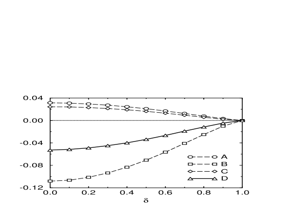
FIG. 1.: The corrections of Eq. (103) at $T=0$. The curves A, B, C, and D represent the functions $K^{\infty}(\delta)$, $K^{II}(\delta)$, $K^{III}(\delta)$, and their sum, respectively.

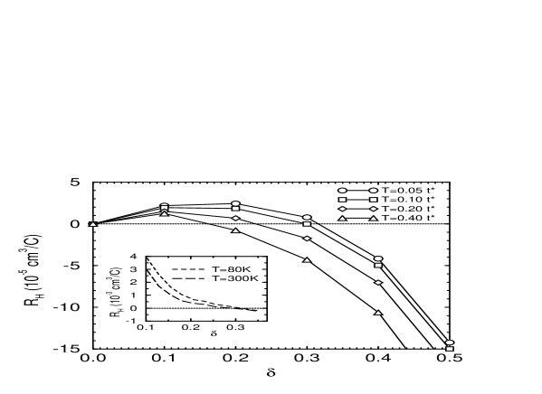
FIG. 2.: Hall constant as a function of doping for $U=2.3\,W$. Inset: Data for polycrystalline samples of La_2-δSr_δCuO₄ taken from Ref. [5].

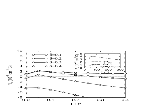
FIG. 3.: Hall constant as a function of temperature for $U=2.3\,W$. Inset: Data for polycrystalline samples of La_2-δSr_δCuO₄ taken from Ref. [11].

REFERENCES

- [1] H. Kohno, K. Yamada, Prog. Theor. Phys. 80, 623 (1988).
- [2] For a review, see N. P. Ong, Physical Properties of High Temperature Superconductors, edited by D. M. Ginsberg, World Scientific, Singapore (1990), Vol. 2.
- [3] B. S. Shastry, B. I. Shraiman, R. P. Singh, Phys. Rev. Lett. 70, 2004 (1993).
- [4] H. Fukuyama, Y. Hasegawa, Physica B 148, 204 (1987).
- [5] H. Takagi et al., Phys. Rev. B 40, 2254 (1989).
- [6] N. P. Ong et al., Phys. Rev. B 35, 8807 (1987).
- [7] N. P. Ong, Phys. Rev. B 43, 193 (1991).
- [8] J. M. Harris, Y. F. Yan, N. P. Ong, Phys. Rev. B 46, 14293 (1992).
- [9] J. M. Ziman, Electrons and Phonons, Oxford (1960).
- [10] T. R. Chien, Z. Z. Wang, N. P. Ong, Phys. Rev. Lett. 67, 2088 (1991).
- [11] H. Y. Hwang et al., Phys. Rev. Lett. 72, 2636 (1994).
- [12] E. Lange, to be published.
- [13] L. Friedman, T. Holstein, Ann. Phys. (N. Y.) 21, 494 (1963); Phys. Rev. 165, 1019 (1968); K. G. Wilson, Phys. Rev. D 10, 2445 (1974).
- [14] E. Fick, G. Sauermann, The Quantum Statistics of Dynamic Processes, Springer (1990).
- [15] D. Forster, Hydrodynamic Fluctuations, Broken Symmetry, and Correlation Functions, Addison-Wesley (1975).
- [16] W. Götze, P. Wölfle, Phys. Rev. B 6, 1226 (1972) and J. Low Temp. Phys. 5, 575 (1971).
- [17] A. L. Fetter, J. D. Walecka, Quantum Theory of Many-Particle Systems, McGraw-Hill (1971).
- [18] W. Metzner, D. Vollhardt, Phys. Rev. Lett. 62, 324 (1989).
- [19] T. Pruschke, T. Obermeier, J. Keller, M. Jarrell, to be published in Physica B.
- [20] A variety of transport properties was investigated within the Hubbard model in including the Hall effect in Ref. [22]. These authors have estimated . However, their treatment of the Hall effect is based on a formula for the Hall conductivity that was derived by neglecting vertex corrections and which is restricted to Lorentzian-shaped spectral functions only [23]. In contrast to this, none of both problems arise in the case of the ordinary conductivity. For instance, its vertex corrections vanish in infinite dimensions [24].
- [21] E. Müller-Hartmann, Z. Phys. B 74, 507 (1989).
- [22] T. Pruschke, M. Jarrell, J. K. Freericks, Adv. Phys. 44, 187 (1995).
- [23] P. Voruganti, A. Golubentsev, S. John, Phys. Rev. B 45, 13945.
- [24] A. Khurana, Phys. Rev. Lett. 64, 1990 (1990).