Low frequency shot noise in double-barrier resonant-tunneling ${\text{G}aAs/Al_{x}Ga_{1-x}As}$ structures in a strong magnetic field

Abstract

Low frequency shot noise and dc current profiles for a double-barrier resonant-tunneling structure (DBRTS) under a strong magnetic field applied perpendicular to the interfaces have been studied. Both the structures with 3D and 2D emitter have been considered. The calculations, carried out with the Keldysh Green’s function technique, show strong dependencies of both the current and noise profiles on the bias voltage and magnetic field. The noise spectrum appears sensitive to charge accumulation due to barriere capacitances and both noise and dc-current are extremely sensitive to the Landau levels’ broadening in the emitter electrode and can be used as a powerful tool to investigate the latter. As an example, two specific shapes of the levels’ broadening have been considered - a semi-elliptic profile resulting from self-consistent Born approximation, and a Gaussian one resulting from the lowest order cumulant expansion.

I Introduction

In recent years, there has been a great interest in resonant tunneling through double-barrier resonant tunneling structures (DBRTS) (Fig. 1). Such structures have been in focus of many experimental and theoretical investigations since its conception by Tsu and Esaki [1] and first realization of negative differential resistance by Sollner et al.[2]. Many important characteristics of DBRTS have been intensely studied, e.g. dc-properties , phonon assisted tunneling, time dependent processes and frequency response. Noise properties of DBRTS have also been studied both experimentally[3] and theoretically[4, 5, 6, 7, 8]. At low temperatures and in the presence of transport current, shot noise is the dominant source of electrical noise. This kind of noise is due to discreteness of the electron charge, and it is sensitive to the degree of correlation between tunneling processes. In general, a correlation leads to an additional frequency dependence of shot noise, as well as to its suppression below the so-called full noise, $S(0)=2e|I_{\text{dc}}|$ (at $T=0$)[9]. Here $S(\omega)$ is the noise spectrum (see the exact definition below), while $I_{\text{dc}}$ is the average dc current. In a mesoscopic conductor having several independent modes of transverse motion (channels), the noise is determined by the partial transmission probabilities $T_{m}$ as[10, 11, 12] $S\propto\sum_{m}T_{m}(1-T_{m})$, while the conductance goes as $G\propto\sum_{m}T_{m}$. Suppression of the shot noise is thus expected in a phase coherent system when the tunneling probabilities are of the order unity for open quantum channels.

Our concern is a DBRTS in a strong magnetic field perpendicular to the interfaces. Magnetic field is an important tool for sample characterization because it leads to the formation of Landau levels, as well as to drastic modification of electron wave functions. We study the situation when the magnetic field ${\bf B}$ is applied parallel to the tunneling current ${\bf I}$, as schematically illustrated in Fig. 1. In such a configuration, the magnetic field leads to an effectively one-dimensional tunneling problem. Consequently, both the dc current and the noise appear extremely sensitive to the details of the density-of-states behavior. We believe that such a sensitivity can provide a powerful tool to investigate details of the Landau levels’ broadening in resonant tunneling structures.

The paper is organized as follows: Section II describes the model Hamiltonian as well as the basic expression from which the current and shot noise profiles will be derived in Section III. In Appendix A and Appendix B the Green’s functions used in our calculations are expanded.

As an example, we consider a GaAs⁺/ Al_0.3Ga_0.7As/ GaAs/ Al_0.3Ga_0.7As/ GaAs⁺ DBRTS, with the barriers’ and the well widths of the order of 40-60 Å. Such structures were extensively studied experimentally. In many cases the barrier height is about 300 meV, and it is assumed that there exists only one quasi-bound state in the well.

II Model and basic expressions

Consider a DBRTS in the presence of an external magnetic field ${\bf B}$ perpendicular to the interfaces which are assumed perfect, ${\bf B}\parallel{\bf I}\parallel{\bf z}$. Within the quantum well, the electron wave function can be expressed as a product of a quasi-bound state $\chi(z)$ times a wave function correspondent to the motion in the $x-y$ plane. Let us denote the energy of the motion in $z$-direction as $\epsilon_{0}$. Under the Landau gauge ${\bf A}=(0,Bx,0)$ the wave functions can be specified by the set of quantum numbers $\alpha=(n,k_{y})$ as

$$\phi_{\alpha}({\bf r})={1\over\sqrt{Ly}}\exp(ik_{y}y)\varphi_{n}(x+l^{2}k_{y})\chi(z).$$ (1)

The corresponding energy levels (measured from the conduction band edge) are

$$E_{\alpha}=E_{n}=\epsilon_{0}+\hbar\omega_{c}(n+\frac{1}{2}).$$ (2)

Here, $\varphi_{n}(x)$ denote harmonic oscillator states, $\omega_{c}\equiv eB/m^{*}$ is the cyclotron frequency, and $l\equiv\sqrt{\hbar/eB}$ is the Landau magnetic length.

Similarly, electron states in the leads are specified by the quantum numbers $\beta=(m,k_{j,y},k_{j,z})$, where $j\equiv e(c)$ refers to emitter(collector) states, respectively. The corresponding wave functions and energy levels under the bias $eV$ are given as:

$$\phi_{j,\beta}({\bf r})={1\over\sqrt{L_{y}L_{z}}}\exp(ik_{j,z}z+ik_{j,y}y)\varphi_{m}(x+l^{2}k_{j,y}),$$ (3)

$$E_{j,\beta}=\frac{(\hbar k_{j,z})^{2}}{2m^{*}}+\hbar\omega_{c}(m+\frac{1}{2})+a_{j}eV$$ (4)

where $0<a_{e}<1$ and $a_{c}=a_{e}-1$ (the symmetric $a_{e}=0.5$ case will be considered in our numerical calculations). We arrive at the model Hamiltonian

$${\cal H}={\cal H}_{\text{e}}+{\cal H}_{\text{T}}=\sum_{j,\beta}E_{j,\beta}c_{j,\beta}^{\dagger}c_{j,\beta}+\sum_{\alpha}E_{\alpha}c_{\alpha}^{\dagger}c_{\alpha}+\sum_{j,\alpha,\beta}\left[V_{j,\beta\alpha}c_{\alpha}^{\dagger}c_{j,\beta}+h.c\right],$$ (5)

where the tunnel matrix elements $V_{j,\beta\alpha}$ have to be calculated using the eigenstates listed above. Since the interfaces are assumed to be perfect, the quantum numbers $n$ and $k_{y}$ are conserved during the tunneling process, and so the calculation of the matrix elements $V_{j,\beta\alpha}$ reduces to the solving of a one-dimensional Schrödinger equation[13], following with the application of the Bardeen’s prescription[14]. Consequently, the tunneling matrix elements can be written as

$$V_{j,\beta\alpha}=\delta_{m,n}\delta(k_{y}-k_{j,y})V_{j,n}(k_{j,y},k_{j,z}).$$ (6)

In noise calculations the time dependence of the tunneling currents flowing through the DBRTS is important, and hence the junction capacitances should be taken into account. The effect of the junction capacitances can be included in our model with the help of an equivalent circuit of the DBRTS as shown in Fig. 2.[15] In this circuit, we specify the currents through the emitter (collector) barriers $I_{\text{e(c)}}(t)$ and their resistances as $R_{\text{e(c)}}$. The “external” current $I(t)$ is in this model given by

$$I(t)={C_{\text{c}}\over C}I_{\text{e}}(t)+{C_{\text{e}}\over C}I_{\text{c}}(t),$$ (7)

where $C_{\text{e(c)}}$ is the capacitance of the emitter (collector) barrier and $C=C_{\text{e}}+C_{\text{c}}$ is the total capacitance of the quantum well. In the symmetric case $C_{\text{e}}=C_{\text{c}}$, we arrive at the simple relation $I(t)=[I_{\text{e}}(t)+I_{\text{c}}(t)]/2$, which was the basis of the Chen & Ting’s[4] calculation for shot noise in a DBRTS in a zero magnetic field. If one ignores the charge accumulation, all three currents are the same[5], $I(t)=I_{\text{e}}(t)=I_{\text{c}}(t)$ and the result in this case can be obtained from the following formulas in the limit of strong asymmetry, $C_{\text{e(c)}}/C\rightarrow 0$. The asymmetry in capacitances is of course not important for the dc-current, where

$$I_{\text{d}c}=I_{\text{d}c,e}=I_{\text{d}c,c}$$ (8)

In the further analysis it is convenient to out $\hbar=1$, and then restore $\hbar$ again in the final expressions and order-of-magnitude estimates.

The tunneling current $I_{\text{e}}$ flowing into the well from the emitter and the current $I_{\text{c}}$ flowing out of the well to the collector, are in general different. They are given by the expressions

$$I_{\text{d}c,j} = -e\kappa_{j}\langle\dot{N}_{j}(t)\rangle=-ie\kappa_{j}\left\langle[{\cal H}_{T}(t),N_{\text{j}}(t)]\right\rangle$$ (9)

$$= -i2e\kappa_{j}\sum_{\beta,\alpha}\left[V_{j,\beta\alpha}\langle c_{\alpha}^{\dagger}(t)c_{j,\beta}(t)\rangle-V_{j,\beta\alpha}^{*}\langle c_{j,\beta}^{\dagger}(t)c_{\alpha}(t)\rangle\right]$$ (10)

where $N_{j}(t)$ are the Heisenberg number-of-particles operators, $\kappa_{e}\equiv 1$, $\kappa_{c}\equiv-1$, and a spin degeneracy factor $2$ is introduced.

The shot noise spectrum is defined as the Fourier transform of the current-current auto-correlation function as[9]

$$S(\omega)=2\int_{-\infty}^{\infty}S(t)e^{i\omega t}dt=4\int_{0}^{\infty}S(t)\cos(\omega t)dt$$ (11)

where $S(t)$ is the quantum mechanical and statistical average of the current-current anti-commutator:

$$S(t)={1\over 2}\left\langle\{\Delta I(t)\,,\,\Delta I(0)\}\right\rangle={1\over 2}\left\langle\{I(t)\,,\,I(0)\}\right\rangle-I_{\text{dc}}^{2}.$$ (12)

From (7) and (9), it can be expressed (having in mind the spin degeneracy factor of 2) as

$$S(t)=-e^{2}\sum_{j,j_{0},\alpha,\alpha_{0},\beta,\beta_{0}}\eta_{j}\eta_{j_{0}} \times \left[V_{j,\beta\alpha}V_{j_{0},\beta_{0}\alpha_{0}}\left\langle\left\{c_{\alpha}^{\dagger}(t)c_{j,\beta}(t),c_{\alpha_{0}}^{\dagger}(0)c_{j_{0},\beta_{0}}(0)\right\}\right\rangle\right.$$ (13)

$$- V_{j,\beta\alpha}V_{j_{0},\beta_{0}\alpha_{0}}^{*}\left\langle\left\{c_{\alpha}^{\dagger}(t)c_{j,\beta}(t),c_{j_{0},\beta_{0}}^{\dagger}(0)c_{\alpha_{0}}(0)\right\}\right\rangle$$ (14)

$$- V_{j,\beta\alpha}^{*}V_{j_{0},\beta_{0}\alpha_{0}}\left\langle\left\{c_{j,\beta}^{\dagger}(t)c_{\alpha}(t),c_{\alpha_{0}}^{\dagger}(0)c_{j_{0},\beta_{0}}(0)\right\}\right\rangle$$ (15)

$$+ \left.V_{j,\beta\alpha}^{*}V_{j_{0},\beta_{0}\alpha_{0}}^{*}\left\langle\left\{c_{j,\beta}^{\dagger}(t)c_{\alpha}(t),c_{j_{0},\beta_{0}}^{\dagger}(0)c_{\alpha_{0}}(0)\right\}\right\rangle\right].$$ (16)

where $\eta_{e}\equiv C_{c}/C$ and $\eta_{c}\equiv-C_{e}/C$. Being expressed through Feynman’s graphs, these averages involve only the diagrams with the Green’s functions connecting the times $t$ and $0$, since disconnected parts are all canceled by the $I_{\text{dc}}^{2}$ subtraction in (12).

III The results

The task is now to expand the quantum statistical averages appearing in (9) and (13). For a finite bias, the DBRTS as a whole is not in thermal equilibrium, and it seems thus appropriate to employ the Keldysh non-equilibrium Green’s function technique[16, 17], where the two lead subsystems are supposed to have their own local equilibrium.

Expanding (9) yields (Appendix A)

$$I_{\text{d}c,j}=-{e\;g_{B}\over\pi}\sum_{n}\int_{-\infty}^{\infty}d\varepsilon\;\gamma_{j}(n,\varepsilon)A(n,\varepsilon)\left[f_{QW}(\varepsilon)-f_{j}(\varepsilon)\right].$$ (17)

In the above expression, $g_{b}\equiv L_{x}\>L_{y}/2\pi l^{2}$ is the magnetic $k_{y}$ summation degeneracy factor, $\gamma_{j}(n,\varepsilon)$ is the escape rate to the lead $j$, $f_{QW}(\varepsilon)$ and $f_{j}(\varepsilon)$ are the occupation factors, while $A(n,\varepsilon)$ is the spectral function for $n$th Landau level in the well,

$$A(n,\varepsilon)=-2\Im G_{R}(n,\varepsilon)={\gamma(n,\varepsilon)\over(\varepsilon-E_{n})^{2}+[\gamma(n,\varepsilon)/2]^{2}}.$$ (18)

Here, $G_{R}(n,\varepsilon)$ is the retarded electron Green’s function, and $\gamma(n,\varepsilon)=\gamma_{e}(n,\varepsilon)+\gamma_{c}(n,\varepsilon)$ is the level broadening due to the finite escape rate to the leads. Usually, the energy distance between the resonant level in the well and the tops of the barriers is much greater than the escape rate from the well, $\gamma$. In this case the tunneling matrix element (6) can be considered as a smooth function of the energy in comparison with the energy dependence of the density-of-states in the leads,

$$g_{j}(n,\varepsilon)\equiv\sum_{k_{j,z}}\delta(\varepsilon-E_{j,\beta}).$$

Thus the escape rates $\gamma_{j}$ can be expressed as

$$\gamma_{j}(n,\varepsilon)=2\pi|V_{j}|^{2}g_{j}(n,\varepsilon).$$

Consequently, the noise appears a sensitive tool to study density-of-states in the electrodes in a magnetic field. Below, we will do numerical calculations for two models for the density of states - for a constant Lorentzian broadening, and for the so-called self-consistent Born approximation.

Since both leads are assumed to be in a thermal equilibrium with different electro-chemical potentials and Fermi energies, the occupation numbers can be expressed as the Fermi functions:

$$f_{j}(\varepsilon)={1\over{e^{(\varepsilon-E_{f}-a_{j}eV)/k_{B}T}+1}}.$$ (19)

However, thermal equilibrium is not maintained in the quantum well and thus one cannot use the Fermi distribution for the electrons in this region. Instead, from the dc-current conservation law (8), the weighed average occupation factor is determined as[18]

$$f_{QW}(n,\varepsilon)={\gamma_{e}(n,\varepsilon)f_{e}(\varepsilon)+\gamma_{c}(n,\varepsilon)f_{c}(\varepsilon)\over\gamma(n,\varepsilon)}.$$ (20)

Re-introducing $\hbar$ to return to the proper units, we arrive at the Landauer formula [19]

$$I_{\text{d}c}={e\;g_{B}\over\pi\hbar}\sum_{n}\int d\varepsilon\;T_{n}(\varepsilon)\left[f_{e}(\varepsilon)-f_{c}(\varepsilon)\right]$$ (21)

with the transmission probability

$$T_{n}(\varepsilon)\equiv{\gamma_{e}(n,\varepsilon)\gamma_{c}(n,\varepsilon)\over\gamma(n,\varepsilon)}A(n,\varepsilon)$$ (22)

To get a relatively simple expressions for the shot noise from Eq. (13) we assume the following approximations. First, we assume that the resonant level is situated well inside the resonant tunneling region,

$$|a_{j}eV_{j}+E_{F}-E_{n}|\gg\max(\hbar\omega,\gamma,\nu_{j}),$$ (23)

$$|a_{j}eV_{j}-\epsilon_{0}|\gg\max(\hbar\omega,\gamma,\nu_{j}),$$ (24)

and that $\omega\ll\omega_{c}$. These inequalities allow us to put $f_{j}(\varepsilon\pm\omega)\rightarrow f_{j}(\varepsilon)$ and $\gamma_{j}(n,\varepsilon\pm\omega)\rightarrow\gamma_{j}(n,\varepsilon)$. Second, the temperature is assumed to be low ($k_{B}T\ll\gamma$), in which case the Fermi functions can be approximated as step functions. Keeping those approximations in mind, we arrive at the following result (Appendix B):

$$S(\omega)=S(-\omega) = {e^{2}\;g_{B}\over\pi}\sum_{n}\int d\varepsilon\left[f_{e}(\varepsilon)-f_{c}(\varepsilon)\right]^{2}\times$$ (25)

$$\times \left\{A(n,\varepsilon)A(n,\varepsilon-\omega)\left[{\gamma_{e}\gamma_{c}(\gamma_{e}C_{e}-\gamma_{c}C_{c})(\gamma_{e}C_{c}-\gamma_{c}C_{e})\over C^{2}\gamma^{2}}-{\gamma_{e}^{2}\gamma_{c}^{2}\over\gamma^{2}}\right]\right.$$ (26)

$$+ \left[A(n,\varepsilon)+A(n,\varepsilon-\omega)\right]{C_{e}^{2}+C_{c}^{2}\over C^{2}}{\gamma_{e}\gamma_{c}\over\gamma}$$ (27)

$$- \left.4\Re\left[G_{R}(n,\varepsilon)\right]\Re\left[G_{R}(n,\varepsilon-\omega)\right]{C_{e}C_{c}\over C^{2}}\gamma_{e}\gamma_{c}\right\}$$ (28)

where $\gamma_{j}\equiv\gamma_{j}(n,\varepsilon)$.

Re-inserting $\hbar$, and using the relation $4\,\gamma_{e}\gamma_{c}\Re\left[G_{R}(n,\varepsilon)\right]^{2}=4\,T_{n}(\varepsilon)-(\gamma^{2}/\gamma_{\text{e}}\gamma_{\text{c}})\;T_{n}^{2}(\varepsilon)$, we arrive at the well known result:

$$S(0)={2e^{2}\;g_{B}\over\pi\hbar}\sum_{n}\int d\varepsilon\;T_{n}(\varepsilon)\left[1-T_{n}(\varepsilon)\right]\left[f_{e}(\varepsilon)-f_{c}(\varepsilon)\right]^{2}$$ (29)

As one could expect, the zero frequency shot noise does thus not depend on the barriere capacitances and the above result coincides with previous calculations which have been performed for point contacts [10, 11], for arbitrary phase coherent two terminal conductors[12] (neglecting barriere capacitances), and also for a DBRTS in the regime of incoherent tunneling[6]. The main features of our problem is that the combinations $T_{n}(1-T_{n})$ enter for each Landau level independently and that the tunneling probabilities $T_{n}$ are strong functions of magnetic field. An important feature is that Eq. (29) holds even if the inequality (23) is violated. That makes zero-frequency shot noise, together with the dc-current, a powerful tool to investigate the density of states in the leads which manifests itself through the escape rates $\gamma_{j}$.

The results for a particular DBRTS device are shown in Fig. 3. Here we use the model of constant Lorentzian broadening of the Landau levels, where the escape rates can be expressed as (Appendix A)

$$\gamma_{j}(n,\varepsilon)={\Upsilon_{j}\;\nu\over 2\sqrt{2}\left\{\left[\left(\varepsilon-E_{j,n}\right)^{2}+\left(\nu/2\right)^{2}\right]\left[\sqrt{\left(\varepsilon-E_{j,n}\right)^{2}+\left(\nu/2\right)^{2}}+E_{j,n}-\varepsilon\right]\right\}^{1/2}}.$$ (30)

Here, $\Upsilon_{j}$ is a constant characterizing the strength of the escape rate and $E_{j,n}\equiv eVa_{j}+\omega_{c}(n+1/2)$. Note that there are peaks in the dimensionless shot noise factor $S(\omega)/eI_{\text{dc}}$ at the voltages when an intra-well Landau level passes the emitter’s electro-chemical potential. Those peak’s shape is determined by an interplay between the quantum suppression ($S(0)\propto T_{n}(1-T_{n})$) and a finite broadening of the Landau levels in the quantum well. In addition, a small peak appears in the dc-current curve at the end of the resonant tunneling region (in our example, at $eV\sim 55$ meV) due to the finite broadening of the lead electron states. This broadening can typically be of the size $\nu\sim\hbar e/m^{*}\mu\sim 0.5$ meV ($\mu$ is the electron mobility).

The effect of the level broadening in the leads is even more pronounced in the case of a 2D-emitter. For numerical calculations in this case we employ the so-called self-consistent Born approximation [20]. In this approximation, the density of states takes a semi-elliptic form and the escape rate is then given by:

$$\gamma_{e}(n,\varepsilon)=\Upsilon_{e}{4\;\hbar\over\sqrt{2m^{*}}L_{ez}\;\nu}\sqrt{1-\left({\varepsilon-E_{e,n}\over\nu}\right)^{2}}.$$ (31)

where $E_{e,n}=eVa_{e}+\omega_{c}(n+1/2)+\epsilon_{e}$, $\epsilon_{e}$ is the emitter quasi-bound level and $L_{ez}$ is the width of the 2D-emitter. The lead broadening depends in this case on the magnetic field and is given by $\nu\sim\sqrt{2\hbar^{2}e\;\omega_{c}/\pi m^{*}\mu}$, where $\mu$ is the mobility of the 2DEG. In our example, $\mu\sim 10^{6}$ cm²/Vs, at $\hbar\omega_{c}=10$ meV we get $\nu\sim 0.35$ meV. In realistic systems, sharp edges of the semi-elliptical density-of-states profile are smoothed, the smoothing for a long-range potential being Gaussian[21]. To check the sensitivity to the smoothing we made also calculations for a Gaussian density-of-states profile. The calculations show that both the current and the noise profiles can be very sensitive to the degree of such a smoothing. Fig. 4 shows the dc-current and zero frequency shot noise results for a particular DBRTS device with 2D emitter calculated according to the self-consistent Born approximation (semi-elliptic profile) as well as for a Gaussian profile obtained from a so-called lowest-order cumulant approximation[20, 22]. A double-peak structure is obtained with the Gaussian profile in contrast to the single peak appearing in the case of a semi-elliptic profile.

We believe that our results can serve as a basis for an experimental test of the strength of the Landau level’s smearing by impurities. In our example, the splitting of the noise and current peaks in the case of the Gaussian level broadening case is about 2 meV, and should be observable at temperatures $T\ll 20$ K.

Finally, we give an expression for the shot noise valid at finite frequency provided the inequality (23) holds. Integrating (21) and (25) with a 3D emitter, we arrive at the expression (Appendix B)

$$S(\omega)={2|eI_{dc}|\over C^{2}}\left\{\left(C_{e}^{2}+C_{c}^{2}\right)+{1\over\gamma^{2}+\omega^{2}}\right. \times \left[C_{e}C_{c}(\gamma_{e}^{2}+\gamma_{c}^{2})-(C_{e}^{2}+C_{e}^{2})\gamma_{e}\gamma_{c}\right.$$ (32)

$$- \left.\left.\gamma_{e}\gamma_{c}C^{2}+C_{e}C_{c}\gamma^{2}\right]\right\}$$ (33)

This result is strongly dependent of the bias voltage because of the voltage dependence of the escape rates. Indeed, at $|\epsilon_{0}-eVa_{j}|\gg\max(\hbar\omega,\gamma,\nu_{j})$,

$$\gamma_{j}\equiv\gamma_{j}(eV)=\Upsilon_{j}{\Theta(\epsilon_{0}-eVa_{j})\over\sqrt{\epsilon_{0}-eVa_{j}}}.$$

As our two special cases, symmetric capacitance ($C_{e}=C_{c}$) and no charge accumulation ($C_{c(e)}\rightarrow 0$), we arrive at the relations similar to those obtained by Chen & Ting[4] and by Büttiker[5] in zero magnetic field:

$$S_{\text{s}ym}(\omega) = \mid eI_{dc}\mid\left[1+{\gamma^{2}\over\gamma^{2}+\omega^{2}}\left(1-4{\gamma_{e}\gamma_{c}\over\gamma^{2}}\right)\right]$$ (34)

$$S_{\text{a}sym}(\omega) = 2\mid eI_{dc}\mid\left[1-2{\gamma_{e}\gamma_{c}\over\gamma^{2}+\omega^{2}}\right].$$ (35)

However, the important difference is strong dependencies of the escape rates on both electric and magnetic fields. The frequency dependency of the noise in those two cases are very different (Fig. 5) and can serve as a basis for an experimental test of the importance of the charge accumulation on the barrier capacitances in the DBRTS tunneling structure.

The present work has partially been supported by the Norwegian Research Council, Grant No. 100267/410.

A Green’s function expansion for dc current

The quantum statistical averages appearing in (9) is expanded using the Keldysh non-equilibrium Green’s function technique[16, 17]. Four different Green’s functions, appropriate for a S-matrix expansion in the time-loop formalism, are defined along a closed time path that runs from $-\infty$ to $+\infty$ along the $\sigma=$‘1’ branch and then returns from $+\infty$ back to $-\infty$ along the $\sigma=$ ‘2’ branch:

$$G_{\sigma_{1}\sigma_{2}}(t_{1}-t_{2})=-i\langle{\cal T}_{t}c(t_{1})c^{\dagger}(t_{2})\rangle$$ (A1)

where by $\sigma_{n}=1(2)$ is meant that $t_{n}$ is located on the ‘1’(‘2’) branch and ${\cal T}_{t}$ is the generalized chronological operator ordering physical operators along the closed time path. In the Fourier transformed energy space, the Green’s functions are simply related to the retarded Green’s functions as:

$$G_{11}(\varepsilon) = if(\varepsilon)A(\varepsilon)+G_{R}(\varepsilon),$$ (A2)

$$G_{12}(\varepsilon) = if(\varepsilon)A(\varepsilon),$$ (A3)

$$G_{21}(\varepsilon) = -i\left[1-f(\varepsilon)\right]A(\varepsilon),$$ (A4)

$$G_{22}(\varepsilon) = -i\left[1-f(\varepsilon)\right]A(\varepsilon)-G_{R}(\varepsilon).$$ (A5)

Here $A(\varepsilon)\equiv-2\Im\left[G_{R}(\varepsilon)\right]$ is the spectral function, while $f(\varepsilon)$ is the occupation number in the region considered. The following retarded quantum well and lead Green’s functions are used as the basis in the calculations:

$$G^{0}_{R}(\alpha,\varepsilon) = [\varepsilon-E_{\alpha}+i\gamma(n,\varepsilon)/2]^{-1},$$ (A6)

$$G^{0}_{R}(j\beta,\varepsilon) = [\varepsilon-E_{j,\beta}+i\nu_{j}/2]^{-1}.$$ (A7)

Here $\gamma(n,\varepsilon)=\gamma_{e}(n,\varepsilon)+\gamma_{c}(n,\varepsilon)$ is the broadening of the resonant states due to the finite tunneling rate to the leads, and $\nu_{j}$ is the broadening of electron states in the leads due to electron scattering.

The dc current is expanded to lowest order in the time-loop S-matrix expansion[17], which from (9) yields (as diagrammatically represented in Fig. 6):

$$I_{\text{dc},j} = -4e\kappa_{j}\lim_{\acute{t}\rightarrow t}\sum_{\alpha,\beta}\int_{-\infty}^{-\infty}dt_{1}\mid V_{j,\beta\alpha}\mid^{2}\Re\left\langle{\cal T}_{t}c_{j,\beta}^{\dagger}(t_{1})c_{\alpha}(t_{1})c_{j,\beta}(t)c_{\alpha}^{\dagger}(\acute{t})\right\rangle$$ (A8)

$$= \quad 4e\sum_{\alpha,\beta}\int_{-\infty}^{\infty}dt_{1}\mid V_{j,\beta\alpha}\mid^{2}\;\Re\left[G_{11}(j\beta,t-t_{1})G_{12}(\alpha,t_{1}-t)\right.$$ (A10)

$$\qquad\qquad\qquad\qquad\qquad\quad\left.-G_{12}(j\beta,t-t_{1})G_{22}(\alpha,t_{1}-t)\right].$$

In the first of the above integrals, $t$ is located on the ‘$1$’ branch, $\acute{t}$ is located on the ‘$2$’ branch and the $t_{1}$ integral is taken along the time-loop from $-\infty$ to $+\infty$ and back to $-\infty$. The latter result, introducing Green’s functions according to (A1), is expressed as an integral over ordinary real time axis from $-\infty$ to $\infty$. The Fourier transform of this result, with the substitution of (A2), yields:

$$I_{\text{d}c,j}=-{e\over\pi}\sum_{\alpha,\beta}\mid V_{j,\beta\alpha}\mid^{2}\int_{-\infty}^{\infty}d\varepsilon\;A(\alpha,\varepsilon)A(j\beta,\varepsilon)\left[f_{QW}(\varepsilon)-f_{j}(\varepsilon)\right],$$ (A11)

where $f_{QW}(\varepsilon)$ and $f_{j}(\varepsilon)$ are respectively the occupation numbers in the quantum well and leads. Using the escape rates from the quantum well states to the lead $j$, defined as

$$\gamma_{j}(n,\varepsilon)=\sum_{k_{j,z}}\mid V_{j}\mid^{2}A(j\beta,\varepsilon)$$ (A12)

where the tunneling matrix elements in (6) have been assumed to be independent on any quantum numbers ($V_{j,n}(k_{y}^{j},k_{z}^{j})=V_{j}$) and taking into account the $k_{y}$ independence of the electron Green’s functions, ($A(\alpha,\varepsilon)=A(n,\varepsilon)$), we arrive at (17) and (30).

B Green’s function expansion for shot noise

The quantum statistical averages appearing in (13) is expanded in a similar way as with the dc current. It is found that $S(\omega)$ is symmetric in $\omega$ and can be written as a sum of 6 different terms (represented by the diagrams in Fig. 7):

$$S(\omega)=S(-\omega)=S_{1}(\omega)+S_{2}(\omega)+S_{3}(\omega)+S_{4}(\omega)+S_{5}(\omega)+S_{6}(\omega).$$ (B1)

$S_{1}(\omega)$ is expanded from the first term in (13) as

$$S_{1}(\omega)=S_{1a}(\omega)+S_{1a}(-\omega)$$ (B2)

with

$$S_{1a}(\omega)= - {e^{2}\over\pi}\sum_{j,j_{0},\alpha,\beta}\eta_{j}\eta_{j_{0}}\mid V_{j}\mid^{2}\mid V_{j_{0}}\mid^{2}\int d\varepsilon\sum_{\sigma_{1},\sigma_{2}}(-1)^{\sigma_{1}+\sigma_{2}}$$ (B3)

$$\times \left[G_{\sigma_{2}1}(\alpha,\varepsilon)G_{2\sigma_{2}}(j\beta,\varepsilon)G_{\sigma_{1}2}(\alpha,\varepsilon-\omega)G_{1\sigma_{1}}(j_{0}\beta,\varepsilon-\omega)\right].$$ (B4)

$S_{2}(\omega)$ is the contribution from the from the 4’th term in (13), simply related to $S_{1}(\omega)$ as

$$S_{2}(\omega)=S_{1}^{*}(\omega).$$ (B5)

The second term in (13) has both zeroth [$S_{3}(\omega)$] and second order [$S_{4}(\omega)$] contributions:

$$S_{3}(\omega) = {e^{2}\over\pi}\sum_{j,\alpha,\beta}\eta_{j}^{2}\mid V_{j}\mid^{2}\int d\varepsilon G_{21}(j\beta,\varepsilon)G_{12}(\alpha,\varepsilon-\omega)+G_{12}(j\beta,\varepsilon)G_{21}(\alpha,\varepsilon-\omega)$$ (B6)

$$S_{4}(\omega) = {e^{2}\over\pi}\sum_{j,j_{0},\alpha,\beta}\eta_{j}\eta_{j_{0}}\mid V_{j}\mid^{2}\mid V_{j_{0}}\mid^{2}\int d\varepsilon\sum_{\sigma_{o}\sigma_{t}=\{12,21\}}\sum_{\sigma_{1},\sigma_{2}}(-1)^{\sigma_{1}+\sigma_{2}}\times$$ (B7)

$$\times \left[G_{\sigma_{1}\sigma_{0}}(j\beta,\varepsilon)G_{\sigma_{2}\sigma_{1}}(\alpha,\varepsilon)G_{\sigma_{t}\sigma_{2}}(j_{0}\beta,\varepsilon)G_{\sigma_{0}\sigma_{t}}(\alpha,\varepsilon-\omega)\right].$$ (B8)

The zeroth [$S_{5}(\omega)$] and second order [$S_{6}(\omega)$] contributions from the third term in (13) are simply given as:

$$S_{5}(\omega)=S_{3}(-\omega)$$ (B9)

$$S_{6}(\omega)=S_{4}(-\omega).$$ (B10)

The diagrams of the type shown in Fig. 8 are not taken into account explicitly because they are already included in $S_{3}(\omega)$ and $S_{5}(\omega)$, since the quantum well electron Green’s functions we use as our basis are originally dressed by tunneling to the leads[7]. Summing up the different diagrammatic terms we neglect the contribution from real part of the lead retarded Green’s functions. This is a reasonable approximation since it corresponds to a Hilbert transform of the imaginary part (proportional to the escape rates) and it appears that, in and above the resonant tunneling region, its contribution is negligible. Keeping this in mind, as well as the approximations listed in the main text ($f_{j}(\varepsilon\pm\omega)\rightarrow f_{j}(\varepsilon)$, $\gamma_{j}(n,\varepsilon\pm\omega)\rightarrow\gamma_{j}(n,\varepsilon)$ and $k_{B}T\ll\gamma$), we arrive at the result (25).

Integrating the shot noise expression (25) and the dc-current (21), we make use of the following integrals over the resonant tunneling region, valid for a Landau level located well inside the resonant tunneling region according to (23):

$$\int d\varepsilon A(n,\varepsilon) \approx 2\pi$$ (B11)

$$\int d\varepsilon A(n,\varepsilon)A(n,\varepsilon-\omega) \approx {4\pi\gamma\over\gamma^{2}+\omega^{2}}$$ (B12)

$$\int d\varepsilon{\text{R}e}\left[G_{R}(n,\varepsilon)\right]{\text{R}e}\left[G_{R}(n,\varepsilon-\omega)\right] \approx {\pi\gamma\over\gamma^{2}+\omega^{2}}.$$ (B13)

With those relations, we arrive at (32).

FIG. 1.: Schematic illustration of the double-barrier resonant tunneling structure (DBRTS).

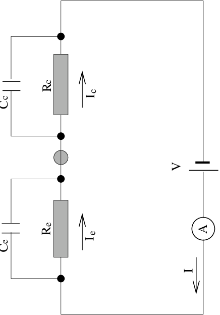
FIG. 2.: Equivalent circuit for a DBRTS.

FIG. 3.: Average current and zero frequency shot noise (A) and dimensionless noise-to-current ratio (B) for a symmetric 3D-emitter DBRTS with: $\Upsilon_{e}=\Upsilon_{c}=0.67$ (meV)^3/2, $\hbar\omega_{c}=10$ meV, $\varepsilon_{0}=27$ meV, $E_{F}=30$ meV and $\nu=0.5$ meV. The shot noise ratio solid curve was obtained from the exact equation (29), while the dashed curve results from the approximation (32).

FIG. 4.: Average urrent and zero frequency shot noise for a symmetrical 2D-emitter DBRTS with: $\Upsilon_{e}=\Upsilon_{c}=0.67$ meV^3/2, $L_{ez}=200\AA$, $\hbar\omega_{c}=10$ meV, $\varepsilon_{0}=27$ meV, $E_{F}=30$ meV, $\epsilon_{e}=10$ meV, $\nu_{3D}=0.5$ meV and $\nu_{2D}=0.35$ meV. A) shows the results obtained from a semi-elliptic Landau level DOS profile in the emitter (see figure inset) while B) shows the corresponding results from a Gaussian DOS profile.

FIG. 5.: Frequency dependence of the noise-to-current ratio for a symmetrical DBRTS with the parameters $\Upsilon_{e}=\Upsilon_{c}=0.67$ meV^3/2, $\hbar\omega_{c}=10$ meV, $\varepsilon_{c}=27$ meV, $E_{F}=30$ meV and with the applied voltage $eV=30$ meV. Curve ‘1’ shows the case of symmetric barrier capacitances (34), while curve ‘2’ is the result when barrier capacitance charge accumulation is negligible (35).

FIG. 6.: Diagrammatic representation for the dc-current Green’s functions.

FIG. 7.: Diagrammatic representation for the noise Green’s functions

FIG. 8.: A typical diagram not taken explicitly into account since it is already implicitly included in other diagrams.

REFERENCES

• [1] R. Tsu and L. Esaki, Appl. Phys. Lett. 22, 562 (1973).
• [2] T. C. L. G. Sollner, W. D. Goodhue, P. E. Tannenwald, C. D. Parker, and D. D. Peck, Appl. Phys. Lett. 43, 588 (1983).
• [3] Y. P. Li, A. Zaslavsky, D. C. Tsui, M. Santos, and M. Shayegan, Phys. Rev. B 41, 8388 (1990).
• [4] L. Y.Chen and C. S. Ting, Phys. Rev. Lett. 43, 4534 (1991).
• [5] M. BΓΌttiker, Phys. Rev. B, 45, 3807 (1992).
• [6] J. H. Davies, P. Hyldgaard, S. Hershfield, and J. Wilkins, Phys. Rev. B 46, 9620 (1992).
• [7] E. Runge, Phys. Rev. B 47, 2003 (1993).
• [8] A.Β LevyΒ Yeyati, F.Β Flores and E.Β V.Β Anda Phys. Rev. B 47, 10543 (1993).
• [9] A. van der Ziel, Noise in Solid State Devices and Circuits (John Wiley & Sons, 1986).
• [10] V. Khlus , Sov.Β Phys. Β JETP 66, 1243, (1987). [Zh.Β Eksp.Β Teor.Β Fiz. 93, 2179 (1987)].
• [11] G. B. Lesovik, JETP Lett. 49, 683, (1989). [Pis’ma Zh.Eksp. Teor. Fiz. 49, 594 (1989)].
• [12] M. BΓΌttiker, Phys. Rev. Lett, 65, 2901 (1990).
• [13] Nanzhi Zou, J. Rammer, and K. A. Chao, Phys. Rev. B 46, 15912 (1992).
• [14] J. Bardeen, Phys. Rev. Lett. 6, 57 (1961).
• [15] G.Β -L.Β Ingold and Yu.Β V.Β Nazarov, in Single charge Tunneling, ed.: H.Β Grabert and M.Β H.Β Devoret. (Plenum New York 1992).
• [16] E. MΒ Lifshitz and L. PΒ Pitaevskii, Physical Kinetics in β€œCourse of Theoretical Physics” Vol.Β 10 (Pergamon Press Ltd., 1981).
• [17] G. D. Mahan, Many Particle Physics (Plenum, New York, 1981).
• [18] M.Β Jonson, Phys.Β Rev.Β B 39, 5924 (1989).
• [19] R. Landauer and Th. Martin, Physica B, 175, 167 (1991)
• [20] T.Β Ando, A. B.Β  Fowler and F.Β Stern, Rev.Β Mod.Β Phys 54, 437 (1982).
• [21] M. E.Β Raikh and T. V.Β Shahbazya, Phys.Β Rev.Β B 47, 1522 (1993).
• [22] R.Β R.Β Gerhards, Surf.Β Sci. 58, 227 (1976).
Refer to caption