Semiclassical theory of shot noise in mesoscopic conductors

Abstract

A semiclassical theory is developed for time-dependent current fluctuations in mesoscopic conductors. The theory is based on the Boltzmann-Langevin equation for a degenerate electron gas. The low-frequency shot-noise power is related to classical transmission probabilities at the Fermi level. For a disordered conductor with impurity scattering, it is shown how the shot noise crosses over from zero in the ballistic regime to one-third of the Poisson noise in the diffusive regime. In a conductor consisting of $n$ tunnel barriers in series, the shot noise approaches one-third of the Poisson noise as $n$ goes to infinity, independent of the transparency of the barriers. The analysis confirms that phase coherence is not required for the occurrence of the one-third suppression of the shot noise. The effects of electron heating and inelastic scattering are calculated, by inserting charge-conserving electron reservoirs between segments of the conductor.

Keywords: Noise and fluctuations, Electronic transport theory

PACS numbers: 73.50.Td, 72.10.Bg, 72.70.+m, 73.23.Ps

I Introduction

The discreteness of the electron charge causes time-dependent fluctuations in the electrical current, known as shot noise. These fluctuations are characterized by a white noise spectrum and persist down to zero temperature. The shot-noise power $P$ contains information on the conduction process, which is not given by the resistance. A well-known example is a vacuum diode, where $P=2e|\bar{I}|\equiv P_{{\rm Poisson}}$, with $\bar{I}$ the average current. This tells us that the electrons traverse the conductor in a completely uncorrelated fashion, as in a Poisson process. In macroscopic samples, the shot noise is averaged out to zero by inelastic scattering.

In the past few years, the shot noise has been investigated in mesoscopic conductors, smaller than the inelastic scattering length. Theoretical analysis shows that the shot noise can be suppressed below $P_{{\rm Poisson}}$, due to correlations in the electron transmission imposed by the Pauli principle [1, 2, 3, 4, 5]. Most intriguingly, it has been found that $P=\frac{1}{3}P_{{\rm Poisson}}$ in a metallic, diffusive conductor [6, 7, 8, 9, 10]. The factor one-third is universal in the sense that it is independent of the material, sample size, or degree of disorder, as long as the length $L$ of the conductor is greater than the mean free path $\ell$ and shorter than the localization length. An observation of suppressed shot noise in a diffusive conductor has been reported [11]. In a quantum mechanical description [6], the suppression follows from the bimodal distribution of transmission eigenvalues [12]. Surprisingly, Nagaev [7] finds the same one-third suppression from a semiclassical approach, in which the Pauli principle is accounted for, but the motion of electrons is treated classically. This implies that phase coherence is not essential for the suppression. A similar conclusion is obtained in Ref. [13]. However, the relationship between the quantum mechanical and semiclassical theories remains unclear [14].

In this paper, we reinvestigate the semiclassical approach and present a detailed comparison with quantum mechanical calculations in the literature. In particular, we study how the shot noise crosses over from the ballistic to the diffusive regime. This complements the study of the crossover of the conductance in Ref. [15]. We use the Boltzmann-Langevin equation [16, 17], which is a semiclassical kinetic equation for nonequilibrium fluctuations. This equation has previously been applied to shot noise by Kulik and Omel’yanchuk [18] for a ballistic point contact, and by Nagaev [7] for a diffusive conductor. Here, we will demonstrate how the Boltzmann-Langevin equation can be applied to an arbitrary mesoscopic conductor. Our analysis corrects previous work by Beenakker and Van Houten [19]. A brief account of our main results has been reported in Ref. [20].

The outline of this paper is as follows: In Section II we discuss the Boltzmann-Langevin equation. It is demonstrated how the shot-noise power can be expressed in terms of semiclassical transmission probabilities. Impurity scattering is treated in Section III. The shot-noise power increases from zero in the ballistic regime to $\frac{1}{3}P_{\rm Poisson}$ in the diffusive regime. We consider both isotropic and nonisotropic impurity scattering, and both a two- and three-dimensional density of states. We also present a one-dimensional model, which can be solved analytically. Exact agreement is found with a previous quantum mechanical evaluation [8], in the limit of a conductance $\gg e^{2}/h$. Section IV deals with barrier scattering. We consider tunneling through $n$ planar barriers in series (tunnel probability $\Gamma$). For $n=2$ and $\Gamma\ll 1$, we recover the results for a double-barrier junction of Refs. [21] and [22]. In the limit $n\rightarrow\infty$ the shot-noise power approaches $\frac{1}{3}P_{{\rm Poisson}}$ independent of $\Gamma$. By taking the continuum limit, $n\rightarrow\infty$, $\Gamma\rightarrow 1$, at fixed $n(1-\Gamma)$, we recover the one-dimensional model of Section III. The case of a disordered region in series with a tunnel barrier concludes Section IV. In Section V we calculate the effects of inelastic scattering and of electron heating due to electron-electron scattering. Analogous to the work of Beenakker and Büttiker [6], this scattering is modeled by putting charge-conserving electron reservoirs between phase-coherent segments of the conductor. This allows us to model the effects of quasi-elastic scattering, electron heating, and inelastic scattering within a single theoretical framework. We conclude in Section VI.

Before proceeding with a description of the semiclassical approach, we briefly summarize the fully quantum mechanical theory. The zero-temperature, zero-frequency shot-noise power $P$ of a phase-coherent conductor is related to the transmission matrix ${\sf t}$ by the formula [4]

$$P=P_{0}\mbox{Tr}\,{\sf t}\,{\sf t}^{\dagger}({\sf 1}-{\sf t}\,{\sf t}^{\dagger})=P_{0}\sum_{n=1}^{N}T_{n}(1-T_{n})\>,$$ (1)

where $P_{0}\equiv 2e|V|G_{0}$, with $V$ the applied voltage and $G_{0}\equiv e^{2}/h$ the conductance quantum (we assume spinless electrons for simplicity of notation), $T_{n}\in[0,1]$ an eigenvalue of ${\sf t}\,{\sf t}^{\dagger}$, and $N$ the number of transverse modes at the Fermi energy $E_{F}$. The conductance is given by the Landauer formula

$$G=G_{0}\mbox{Tr}\,{\sf t}\,{\sf t}^{\dagger}=G_{0}\sum_{n=1}^{N}T_{n}\>.$$ (2)

If the conductor is such that all $T_{n}\ll 1$ (e.g., a high tunnel barrier), one finds $P=2e|V|G\equiv P_{{\rm Poisson}}$, corresponding to a Poisson distribution of the emitted electrons. It has been demonstrated by Levitov and Lesovik [23] (see also Ref. [24]) that the general formula (1) corresponds to a binomial (or Bernoulli) distribution of the emitted electrons for each transmission eigenstate. If some $T_{n}$ are near 1 (open channels), then the shot noise is reduced below $P_{{\rm Poisson}}$. This implies that in a quantum point contact the shot noise is absent on the plateaus of conductance quantization and appears only at the steps between the plateaus [2]. This effect has indeed been observed in experiments [25, 26, 27]. In a metallic, diffusive conductor the $T_{n}$ are either exponentially small or of order unity [12]. This bimodal distribution is required by Ohm’s law for the average conductance [28] and has been derived microscopically by Nazarov [9] and by Altshuler, Levitov, and Yakovets [10]. As a consequence of the bimodal distribution, the shot-noise power is reduced to one-third of the Poisson noise [6].

It has been emphasized by Landauer [29], that Coulomb interactions may induce a further reduction of $P$. Here, we follow the quantum mechanical treatments in assuming noninteracting electrons, within the framework of the Boltzmann-Langevin approach. We do include the effects of electrostatic potential fluctuations in Section V.

II Boltzmann-Langevin equation

We begin by formulating the semiclassical kinetic theory [16, 17]. We consider a conductor with a $d$-dimensional density of states connected by ideal leads to two electron reservoirs (see Fig. 1). The reservoirs have a temperature $T_{0}$ and a voltage difference $V$. The electrons in the left and the right reservoir are in equilibrium, with distribution function, $f_{L}(\varepsilon)=f_{0}(\varepsilon-eV)$ and $f_{R}(\varepsilon)=f_{0}(\varepsilon)$, respectively. Here $f_{0}$ is the Fermi-Dirac distribution,

$$f_{0}(\varepsilon)=\left[1+\exp\left(\frac{\varepsilon-E_{F}}{T_{0}}\right)\right]^{-1}\>.$$ (3)

The fluctuating distribution function $f({\bf r},{\bf k},t)$ in the conductor equals $(2\pi)^{d}$ times the density of electrons with position ${\bf r}$, and wave vector ${\bf k}$, at time $t$. [The factor $(2\pi)^{d}$ is introduced so that $f$ is the occupation number of a unit cell in phase space.] The average over time-dependent fluctuations $\langle f\rangle\equiv\bar{f}$ obeys the Boltzmann equation,

$$\left(\frac{d}{dt}+{\cal S}\right)\bar{f}({\bf r},{\bf k},t)=0\>,$$ (5)

$$\frac{d}{dt}\equiv\frac{\partial}{\partial t}+{\bf v}\cdot\frac{\partial}{\partial{\bf r}}+{\cal F}\cdot\frac{\partial}{\hbar\partial{\bf k}}\>.$$ (6)

The derivative (6) (with ${\bf v}=\hbar{\bf k}/m$) describes the classical motion in the force field ${\cal F}({\bf r})=-e\partial\phi({\bf r})/\partial{\bf r}+e{\bf v}\times{\bf B}({\bf r})$, with electrostatic potential $\phi({\bf r})$ and magnetic field ${\bf B}({\bf r})$. The term ${\cal S}\bar{f}$ accounts for the stochastic effects of scattering. Only elastic scattering is taken into account and electron-electron scattering is disregarded. In the case of impurity scattering, the scattering term in the Boltzmann equation (3) is given by

$${\cal S}f({\bf r},{\bf k},t) = \int d{\bf k}^{\prime}\,W_{{\bf k}{\bf k}^{\prime}}({\bf r})\left\{f({\bf r},{\bf k},t)[1-f({\bf r},{\bf k}^{\prime},t)]-f({\bf r},{\bf k}^{\prime},t)[1-f({\bf r},{\bf k},t)]\right\}$$ (7)

$$= \int d{\bf k}^{\prime}\,W_{{\bf k}{\bf k}^{\prime}}({\bf r})[f({\bf r},{\bf k},t)-f({\bf r},{\bf k}^{\prime},t)]\>.$$ (8)

Here, $W_{{\bf k}{\bf k}^{\prime}}({\bf r})$ is the transition rate for scattering from ${\bf k}$ to ${\bf k}^{\prime}$, which may in principle also depend on ${\bf r}$. [We assume inversion symmetry, so that $W_{{\bf k}{\bf k}^{\prime}}({\bf r})=W_{{\bf k}^{\prime}{\bf k}}({\bf r})$.]

We consider the stationary situation, where $\bar{f}$ is independent of $t$. The time-dependent fluctuations $\delta f\equiv f-\bar{f}$ satisfy the Boltzmann-Langevin equation [16, 17],

$$\left(\frac{d}{dt}+{\cal S}\right)\delta f({\bf r},{\bf k},t)=j({\bf r},{\bf k},t)\>,$$ (9)

where $j$ is a fluctuating source term representing the fluctuations induced by the stochastic nature of the scattering. The flux $j$ has zero average, $\langle j\rangle=0$, and covariance

$$\langle j({\bf r},{\bf k},t)\,j({\bf r}^{\prime},{\bf k}^{\prime},t^{\prime})\rangle=(2\pi)^{d}\,\delta({\bf r}-{\bf r^{\prime}})\,\delta(t-t^{\prime})J({\bf r},{\bf k},{\bf k}^{\prime})\>.$$ (10)

The delta functions ensure that fluxes are only correlated if they are induced by the same scattering process. The flux correlator $J$ depends on the type of scattering and on $\bar{f}$, but not on $\delta f$. The correlator $J$ for the impurity-scattering term (8) has been derived by Kogan and Shul’man [17],

$$J({\bf r},{\bf k},{\bf k^{\prime}}) = -W_{{\bf k}{\bf k}^{\prime}}({\bf r})\left[\bar{f}(1-\bar{f}^{\prime})+\bar{f}^{\prime}(1-\bar{f})\right]$$ (11)

$$+ \delta({\bf k}-{\bf k}^{\prime})\int d{\bf k}^{\prime\prime}\,W_{{\bf k}{\bf k}^{\prime\prime}}({\bf r})\left[\bar{f}(1-\bar{f}^{\prime\prime})+\bar{f}^{\prime\prime}(1-\bar{f})\right]\>,$$ (12)

where $\bar{f}\equiv\bar{f}({\bf r},{\bf k})$, $\bar{f}^{\prime}\equiv\bar{f}({\bf r},{\bf k}^{\prime})$, and $\bar{f}^{\prime\prime}\equiv\bar{f}({\bf r},{\bf k}^{\prime\prime})$. One verifies that

$$\int\!d{\bf k}\,J({\bf r},{\bf k},{\bf k}^{\prime})=\int\!d{\bf k}^{\prime}\,J({\bf r},{\bf k},{\bf k}^{\prime})=0\>,$$ (13)

as it should, since the fluctuating source term conserves the number of particles [$\int d{\bf k}\,j({\bf r},{\bf k},t)=0$]. For the derivation of Eq. (12) we refer to Ref. [17]. In Section IV we give a similar derivation for $J$ in the case of barrier scattering.

Since $j$ and $j^{\prime}$ are uncorrelated for $t>t^{\prime}$, it follows from Eq. (9) that the correlation function $\langle\delta f\,\delta f^{\prime}\rangle$ satisfies a Boltzmann equation in the variables ${\bf r},{\bf k},t$,

$$\left(\frac{d}{dt}+{\cal S}\right)\langle\delta f({\bf r},{\bf k},t)\,\delta f({\bf r}^{\prime},{\bf k}^{\prime},t^{\prime})\rangle=0\>.$$ (14)

Equation (14) forms the starting point of the method of moments of Gantsevich, Gurevich, and Katilius [30]. This method is very convenient to study equilibrium fluctuations, because the equal-time correlation is known,

$$\langle\delta f({\bf r},{\bf k},t)\delta f({\bf r}^{\prime},{\bf k}^{\prime},t)\rangle_{\rm equilibrium}=(2\pi)^{d}\,\bar{f}({\bf r},{\bf k})[1-\bar{f}({\bf r},{\bf k})]\,\delta({\bf k}-{\bf k^{\prime}})\,\delta({\bf r}-{\bf r^{\prime}})\>,$$ (15)

and Eq. (14) can be used to compute the non-equal-time correlation. (For a study of thermal noise within this approach, see, for example, Ref. [31].) Out of equilibrium, Eq. (15) does not hold, except in the reservoirs, and one has to return to the full Boltzmann-Langevin equation (9) to determine the shot noise. In particular, it is only in equilibrium that the equal-time correlation $\langle\delta f\,\delta f^{\prime}\rangle$ vanishes for ${\bf r}\neq{\bf r^{\prime}}$, ${\bf k}\neq{\bf k^{\prime}}$. Out of equilibrium, scattering correlates fluctuations $\delta f$ at different momenta and different points in space.

To obtain the shot-noise power we compute the current $I(t)\equiv\bar{I}+\delta I(t)$ through a cross section $S_{R}$ in the right lead. The average current $\bar{I}$ and the fluctuations $\delta I(t)$ are given by

$$\bar{I}=\frac{e}{(2\pi)^{d}}\int\limits_{S_{R}}\!\!d{\bf y}\int\!d{\bf k}\>v_{x}\,\bar{f}({\bf r},{\bf k})\>,$$ (16)

$$\delta I(t)=\frac{e}{(2\pi)^{d}}\int\limits_{S_{R}}\!\!d{\bf y}\int\!d{\bf k}\>v_{x}\,\delta f({\bf r},{\bf k},t)\>.$$ (17)

We denote ${\bf r}=(x,{\bf y})$, with the $x$-coordinate along and ${\bf y}$ perpendicular to the wire (see Fig. 1). The zero-frequency noise power is defined as

$$P\equiv 2\int\limits_{-\infty}^{\infty}\!\!dt\,\langle\delta I(t)\,\delta I(0)\rangle\>.$$ (18)

The formal solution of Eq. (9) is

$$\delta f({\bf r},{\bf k},t)=\int\limits_{-\infty}^{t}\!\!dt^{\prime}\int\!d{\bf r}^{\prime}\int\!d{\bf k}^{\prime}\,{\cal G}({\bf r},{\bf k};{\bf r}^{\prime},{\bf k}^{\prime};t-t^{\prime})\,j({\bf r}^{\prime},{\bf k}^{\prime},t^{\prime})\>,$$ (19)

where the Green’s function $\cal G$ is a solution of

$$\left(\frac{d}{dt}+{\cal S}\right){\cal G}({\bf r},{\bf k};{\bf r}^{\prime},{\bf k}^{\prime};t)=\delta({\bf r}-{\bf r}^{\prime})\,\delta({\bf k}-{\bf k}^{\prime})\,\delta(t)\>,$$ (20)

such that ${\cal G}=0$ if $t<0$. The transmission probability $T({\bf r},{\bf k})$ is the probability that an electron at $({\bf r},{\bf k})$ leaves the wire through the right lead. It is related to ${\cal G}$ by

$$T({\bf r},{\bf k})=\int\limits_{0}^{\infty}\!\!dt\int\limits_{S_{R}}\!\!d{\bf y}^{\prime}\int\!d{\bf k}^{\prime}\,v_{x}^{\prime}\,{\cal G}({\bf r}^{\prime},{\bf k}^{\prime};{\bf r},{\bf k};t)\>.$$ (21)

Substitution of Eqs. (17) and (19) into Eq. (18) yield for the noise power the expression

$$P = \frac{2e^{2}}{(2\pi)^{2d}}\int\limits_{S_{R}}\!\!d{\bf y}\int\!d{\bf k}\>v_{x}\,\int\limits_{S_{R}}\!\!d{\bf y^{\prime}}\int\!d{\bf k^{\prime}}\>v^{\prime}_{x}\,\int\limits_{-\infty}^{t}\!\!dt^{\prime\prime}\int\!d{\bf r}^{\prime\prime}\int\!d{\bf k}^{\prime\prime}\,{\cal G}({\bf r},{\bf k};{\bf r}^{\prime\prime},{\bf k}^{\prime\prime};t-t^{\prime\prime})\,$$ (22)

$$\times \int\limits_{-\infty}^{0}\!\!dt^{\prime\prime\prime}\int\!d{\bf r}^{\prime\prime\prime}\int\!d{\bf k}^{\prime\prime\prime}\,{\cal G}({\bf r^{\prime}},{\bf k^{\prime}};{\bf r}^{\prime\prime\prime},{\bf k}^{\prime\prime\prime};-t^{\prime\prime\prime})\,\langle j({\bf r^{\prime\prime}},{\bf k^{\prime\prime}},t^{\prime\prime})j({\bf r}^{\prime\prime\prime},{\bf k}^{\prime\prime\prime},t^{\prime\prime\prime})\rangle\>,$$ (23)

which can be simplified using Eqs. (10) and (21):

$$P=\frac{2e^{2}}{(2\pi)^{d}}\int\!d{\bf r}\!\int\!d{\bf k}\!\int\!d{\bf k}^{\prime}\,T({\bf r},{\bf k})\,T({\bf r},{\bf k}^{\prime})J({\bf r},{\bf k},{\bf k}^{\prime})\>.$$ (24)

Equation (24) applies generally to any conductor. It contains the noise due to the current fluctuations induced by the scattering processes inside the conductor. At non-zero temperatures, there is an additional source of noise from fluctuations which originate from the reservoirs. In Appendix A it is shown how this thermal noise can be incorporated. In what follows, we restrict to zero temperature.

A final remark concerns the $x$-coordinate of the cross section at which the current is evaluated [at $x=x_{R}$ in Eq. (17)]. From current conservation it follows that the zero-frequency noise power should not depend on the specific value of $x$. This is explicitly proven in Appendix B, as a check on the consistency of the formalism.

III Impurity scattering

In this Section we specialize to elastic impurity scattering in a conductor made of a material with a spherical Fermi surface and in which the force field ${\cal F}=0$ (so we do not consider the case that a magnetic field is present). The conductor has a length $L$ and a constant width $W$ ($d=2$) or a constant cross-sectional area $A$ ($d=3$). (In general expressions, both $W$ and $A$ will be denoted by $A$.) We calculate the shot noise at zero temperature and small applied voltage, $eV\ll E_{F}$, so that we need to consider electrons at the Fermi energy only. The case of non-zero temperature is briefly discussed in Appendix A.

It is useful to change variables from wave vector $\bf k$ to energy $\varepsilon=\hbar^{2}k^{2}/2m$, and unit vector ${\bf\hat{n}}\equiv{\bf k}/k$. The integrations are modified accordingly,

$$\int\frac{d{\bf k}}{(2\pi)^{d}}\rightarrow\int d\varepsilon\,{\cal D}(\varepsilon)\int\frac{d{\bf\hat{n}}}{s_{d}}\>,$$ (25)

where ${\cal D}(\varepsilon)=s_{d}m(k/2\pi)^{d-2}h^{-2}$ is the density of states, and $s_{d}$ is the surface of a $d$-dimensional unit sphere ($s_{1}=2,\;s_{2}=2\pi,\;s_{3}=4\pi$). We consider the case of specular boundary scattering and assume that the elastic impurity-scattering rate $W_{{\bf k}{\bf k}^{\prime}}({\bf r})\equiv W_{{\bf\hat{n}}{\bf\hat{n}}^{\prime}}\delta(\varepsilon-\varepsilon^{\prime})/{\cal D}(\varepsilon)$ is independent of ${\bf r}$. This allows us to drop the transverse coordinate $\bf y$ and write $T({\bf r},{\bf k})=T(x,{\bf\hat{n}})$ for the transmission probability at the Fermi level. From Eqs. (20) and (21) we derive a Boltzmann equation for the transmission probability [15],

$$v_{F}\,n_{x}\,\frac{\partial T(x,{\bf\hat{n}})}{\partial x} = {\cal S}T(x,{\bf\hat{n}})\>$$ (27)

$$= \int\frac{d{\bf\hat{n}}^{\prime}}{s_{d}}\,W_{{\bf\hat{n}}{\bf\hat{n}}^{\prime}}\,[T(x,{\bf\hat{n}})-T(x,{\bf\hat{n}}^{\prime})]\>.$$ (28)

The boundary conditions in the left and the right leads are

$$T(0,{\bf\hat{n}}) = 0\>,\;\mbox{ if }n_{x}<0\>,$$ (29)

$$T(L,{\bf\hat{n}}) = 1\>,\;\mbox{ if }n_{x}>0\>,$$ (30)

where $x_{L}=0$ and $x_{R}=L$ are the $x$-coordinates of the left and right cross section $S_{L}$ and $S_{R}$, respectively.

The average distribution function can be expressed as

$$\bar{f}({\bf r},{\bf k})=[1-T({\bf r},-{\bf k})]f_{L}(\varepsilon)+T({\bf r},-{\bf k})f_{R}(\varepsilon)\>,$$ (31)

where (because of time-reversal symmetry in the absence of a magnetic field) $T({\bf r},-{\bf k})$ equals the probability that an electron at $({\bf r},{\bf k})$ has arrived there from the right reservoir. Combining Eqs. (16) and (31), we obtain the semiclassical Landauer formula for the linear-response conductance $G\equiv\lim_{V\rightarrow 0}\bar{I}/V$ [32],

$$G = \frac{e^{2}}{(2\pi)^{d}}\int\limits_{S_{x}}\!\!d{\bf y}\int\!d{\bf k}\,\left(\!-\frac{\partial f_{0}(\varepsilon)}{\partial\varepsilon}\right)v_{x}\,T({\bf r},{\bf k})$$ (32)

$$= e^{2}\int\limits_{S_{x}}\!\!d{\bf y}\int d\varepsilon\,{\cal D}(\varepsilon)\left(\!-\frac{\partial f_{0}(\varepsilon)}{\partial\varepsilon}\right)\int\frac{d{\bf\hat{n}}}{s_{d}}\,v\,n_{x}\,T(x,{\bf\hat{n}})$$ (33)

$$= G_{0}N\int\frac{d{\bf\hat{n}}}{v_{d-1}}\,n_{x}\,T(x,{\bf\hat{n}})\>,$$ (34)

with $S_{x}$ the cross section at $x$. The number of transverse modes $N=v_{d-1}(k_{F}/2\pi)^{d-1}A$, where $v_{d}$ is the volume of a $d$-dimensional unit sphere ($v_{0}=1,\;v_{1}=2,\;v_{2}=\pi$). One has $N=k_{F}W/\pi$ for $d=2$ and $N=k_{F}^{2}A/4\pi$ for $d=3$. One can verify that the conductance in Eq. (34) is independent of the value of $x$, as it should: By integrating Eq. (28) over $\bf\hat{n}$ one finds that

$$\frac{\partial}{\partial x}\int d{\bf\hat{n}}\,n_{x}\,T(x,{\bf\hat{n}})=0\>.$$ (35)

We evaluate the noise power by substitution of Eqs. (12) and (31) into Eq. (24). Some intermediate steps are given in Appendix A. The resulting zero-temperature shot-noise power is

$$P=\frac{P_{0}N}{v_{F}s_{d}v_{d-1}}\int\limits_{0}^{L}\!\!dx\int\!\!d{\bf\hat{n}}\int\!\!d{\bf\hat{n}}^{\prime}\,W_{{\bf\hat{n}}{\bf\hat{n}}^{\prime}}\,[T(x,{\bf\hat{n}})-T(x,{\bf\hat{n}}^{\prime})]^{2}T(x,-{\bf\hat{n}})[1-T(x,-{\bf\hat{n}}^{\prime})]\>.$$ (36)

This completes our general semiclassical theory. What remains is to compute the transmission probabilities from Eqs. (25) for a particular choice of the scattering rate $W$. Comparing Eqs. (2) and (34), we note that $\sum_{n}T_{n}$ corresponds semiclassically to $N\int d{\bf\hat{n}}\,n_{x}T(x,{\bf\hat{n}})$. Comparison of Eqs. (1) and (36) shows that the semiclassical correspondence to $\sum_{n}T_{n}(1-T_{n})$ is much more complicated, as it involves the transmission probabilities $T(x,{\bf\hat{n}})$ at all scatterers inside the conductor (and not just the transmission probability $T(0,{\bf\hat{n}})$ through the whole conductor).

In a ballistic conductor, where impurity scattering is absent, the transmission probabilities are given by $T(x,{\bf\hat{n}})=1$, if $n_{x}>0$, and $T(x,{\bf\hat{n}})=0$, if $n_{x}<0$. From Eq. (34), we then obtain the Sharvin conductance $G_{S}\equiv G_{0}N$ [33]. Equation (36) implies that the shot-noise power is zero, in agreement with a previous semiclassical calculation by Kulik and Omel’yanchuk [18].

We now restrict ourselves to the case $W_{{\bf\hat{n}}{\bf\hat{n}}^{\prime}}=v_{F}/\ell$ of isotropic impurity scattering. Let us first show that in the diffusive limit ($\ell\ll L$) the result of Nagaev [7] is recovered. For a diffusive wire the solution of Eq. (34) can be approximated by

$$T(x,{\bf\hat{n}})=\frac{x+\ell\,n_{x}}{L}\>.$$ (37)

Deviations from this approximation only occur within a thin layer, of order $\ell$, at the ends $x=0$ and $x=L$. Substitution of Eq. (37) into Eq. (34) yields the Drude conductance

$$G_{D}=G_{0}N\,\frac{\tilde{\ell}}{L}\>,$$ (38)

with the normalized mean free path $\tilde{\ell}\equiv(v_{d}/v_{d-1})\ell$, i.e. for $d=2$ we have $\tilde{\ell}=\frac{1}{2}\pi\ell$ and for $d=3$ we have $\tilde{\ell}=\frac{4}{3}\ell$. For the shot-noise power we obtain from Eq. (36), neglecting terms of order $(\ell/L)^{2}$,

$$P=P_{0}N\frac{2\tilde{\ell}}{L}\int\limits_{0}^{L}\frac{dx}{L}\,\frac{x}{L}(1-\frac{x}{L})=\frac{1}{3}P_{\rm Poisson}\>,$$ (39)

in agreement with Nagaev [7]. This result is a direct consequence of the linear dependence of the transmission probability (37) on $x$, which is generic for diffusive transport. In Appendix C it is demonstrated that for a diffusive conductor with arbitrary (nonisotropic) impurity scattering $W_{{\bf\hat{n}}{\bf\hat{n}}^{\prime}}$, the result $P=\frac{1}{3}P_{\rm Poisson}$ remains valid.

We can go beyond Ref. [7] and apply our method to quasi-ballistic conductors, for which $\ell$ and $L$ become comparable. In Ref. [15], we showed how in this case the probability $T(x,{\bf\hat{n}})$ can be calculated numerically by solving Eq. (25). With this numerical solution as input, we compute the conductance and the shot-noise power from Eqs. (34) and (36). The result is shown in Fig. 2. The conductance crosses over from the Sharvin conductance to the Drude conductance with increasing length [15]. This crossover is accompanied by a rise in the shot noise, from zero to $\frac{1}{3}P_{\rm Poisson}$. We note small differences between the two and the three-dimensional case in the crossover regime. The crossover is only weakly dependent on the dimensionality of the Fermi surface.

The dimensions $d=2$ and 3 require a numerical solution of Eqs. (25). For $d=1$ an analytical solution is possible. We emphasize that this is not a model for true one-dimensional transport, where quantum interference leads to localization if $L>\ell$ [34]. The case $d=1$ should rather be considered as a toy model, which displays similar behavior as the two and three-dimensional cases, but which allows us to evaluate both the conductance and the shot-noise power analytically for arbitrary ratio $\ell/L$. In the case $d=1$ an electron can move either forward or backward, so $n_{x}\equiv n$ is either 1 or $-1$. The solution of Eq. (25) is

$$T(x,n)=\frac{x+\ell(n+1)}{L+2\ell}\>.$$ (40)

Substitution into Eq. (34) yields

$$G=G_{0}N\,\frac{1}{1+L/\tilde{\ell}}\>,$$ (41)

where $\tilde{\ell}\equiv 2\ell$. Note that the resistance $1/G$ is precisely the sum of the Drude and the Sharvin resistance. The shot-noise power follows from Eq. (36),

$$P = P_{0}N\,\frac{\frac{2}{3}\ell L^{3}+4\ell^{2}L^{2}+8\ell^{3}L}{(L+2\ell)^{4}}$$ (42)

$$= \frac{1}{3}\left(1-\frac{1}{(1+L/\tilde{\ell})^{3}}\right)P_{{\rm Poisson}}\>.$$ (43)

In Fig. 2 we have plotted $G$ and $P$ according to Eqs. (41) and (43). The difference with $d=2$ and $d=3$ is very small.

Liu, Eastman, and Yamamoto [35] have carried out Monte Carlo simulations of the shot noise in a mesoscopic conductor, in good agreement with Eq. (43). In Ref. [8], we have performed a quantum mechanical study of the shot noise in a wire geometry, on the basis of the Dorokhov-Mello-Pereyra-Kumar equation [36]. The semiclassical results for $d=1$ obtained in the present paper, both for the conductance and for the shot-noise power, coincide precisely with these quantum mechanical results, in the limit $N\tilde{\ell}/L\gg 1$. Corrections (of order $P_{0}$) to the shot-noise power, due to weak localization [8], are beyond the semiclassical approach.

IV Barrier scattering

We now specialize to the case that the scattering is due to $n$ planar tunnel barriers in series, perpendicular to the $x$-direction (see inset of Fig. 3). Barrier $i$ has tunnel probability $\Gamma_{i}\in[0,1]$, which for simplicity is assumed to be $\bf k$ and ${\bf y}$-independent. In what follows, we again drop the $\bf y$-coordinate. Upon transmission $\bf k$ is conserved, whereas upon reflection ${\bf k}\rightarrow\widetilde{\bf k}\equiv(-k_{x},{\bf k}_{y})$. At barrier $i$ (at $x=x_{i}$) the average densities $\bar{f}$ on the left side ($x_{i-}$) and on the right side ($x_{i+}$) are related by

$$\bar{f}(x_{i+},{\bf k}) = \Gamma_{i}\bar{f}(x_{i-},{\bf k})+(1-\Gamma_{i})\bar{f}(x_{i+},\widetilde{\bf k})\>,\>\mbox{ if }\>k_{x}>0\>,$$ (45)

$$\bar{f}(x_{i-},{\bf k}) = \Gamma_{i}\bar{f}(x_{i+},{\bf k})+(1-\Gamma_{i})\bar{f}(x_{i-},\widetilde{\bf k})\>,\>\mbox{ if }\>k_{x}<0\>.$$ (46)

To determine the correlator $J$ in Eq. (10), we argue in a similar way as in Ref. [5]. Consider an incoming state from the left $(x_{i-},{\bf k})$ and from the right $(x_{i+},\widetilde{\bf k})$ (we assume $k_{x}>0$). We need to distinguish between four different situations:

1. Both incoming states empty, probability $[1-\bar{f}(x_{i-},{\bf k})][1-\bar{f}(x_{i+},\widetilde{\bf k})]$. Since no fluctuations in the outgoing states are possible, the contribution to $J$ is zero.

2. Both incoming states occupied, probability $\bar{f}(x_{i-},{\bf k})\,\bar{f}(x_{i+},\widetilde{\bf k})$. Again, no contribution to $J$.

3. Incoming state from the left occupied and from the right empty, probability $\bar{f}(x_{i-},{\bf k})[1-\bar{f}(x_{i+},\widetilde{\bf k})]$. On the average, the outgoing states at the left and right have occupation $1-\Gamma_{i}$ and $\Gamma_{i}$, respectively. However, since the incoming electron is either transmitted or reflected, the instantaneous occupation of the outgoing states differs from the average occupation. Upon transmission, the state at the right (left) has an excess (deficit) occupation of $1-\Gamma_{i}$. Upon reflection, the state at the right (left) has an deficit (excess) occupation of $\Gamma_{i}$. Since transmission occurs with probability $\Gamma_{i}$ and reflection with probability $1-\Gamma_{i}$, the equal-time correlation of the occupations is given by

   $$\langle\delta f({\bf r},{\bf k},t)\,\delta f({\bf r}^{\prime},{\bf k}^{\prime},t)\rangle=\left\{\begin{array}[]{l}(2\pi)^{d}\,\Gamma_{i}(1-\Gamma_{i})\,\delta({\bf k}-{\bf k^{\prime}})\,\delta({\bf r}-{\bf r}^{\prime})\>,\\ \;\;\;\vphantom{\int\limits_{0}^{L}}\mbox{ if }\;\;x,x^{\prime}>x_{i}\>\mbox{ or }\>x,x^{\prime}<x_{i}\>,\\ -(2\pi)^{d}\,\Gamma_{i}(1-\Gamma_{i})\,\delta({\bf k}-\widetilde{\bf k}^{\prime})\delta({\bf y}-{\bf y}^{\prime})\,\delta(x+x^{\prime}-2x_{i})\>,\\ \;\;\;\vphantom{\int\limits^{L}}\mbox{ if }\;\;x<x_{i}<x^{\prime}\>\mbox{ or }\>x^{\prime}<x_{i}<x\>,\end{array}\right.$$ (47)

   In terms of the fluctuating source, the fluctuating occupation number can be expressed as

   $$\delta f({\bf r},{\bf k},t)=\frac{1}{|v_{x}|}\int dx_{0}\,j\!\!\left(x_{0},{\bf y}-\frac{{\bf v}_{y}}{v_{x}}\,(x-x_{0}),{\bf k},t-\frac{x-x_{0}}{v_{x}}\right)\>,$$ (48)

   where we have used Eq. (19). (This result is valid as long as only one scattering event has occurred.) Combining Eqs. (47) and (48), it is found that

   $$\langle j({\bf r},{\bf k},t)\,j({\bf r}^{\prime},{\bf k}^{\prime},t^{\prime})\rangle = (2\pi)^{d}\,\Gamma_{i}(1-\Gamma_{i})\,\delta(x-x_{i})\,|v_{x}|\,\delta({\bf r}-{\bf r}^{\prime})$$ (49)

   $$\times [\delta({\bf k}-{\bf k^{\prime}})-\delta({\bf k}-\widetilde{\bf k}^{\prime})]\,\delta(t-t^{\prime})\>,$$ (50)

   upon the initial condition of occupied left and unoccupied right incoming state.

4. Incoming state from the left unoccupied and from the right occupied, probability $[1-\bar{f}(x_{i-},{\bf k})]\bar{f}(x_{i+},\widetilde{\bf k})$. Similar to situation (c).

Collecting results from (a)–(d) and summing over all barriers, we find

$$J(x,{\bf k},{\bf k}^{\prime}) = \sum_{i=1}^{n}\delta(x-x_{i})\,\Gamma_{i}(1-\Gamma_{i})\,|v_{x}|\,[\delta({\bf k}-{\bf k}^{\prime})-\delta({\bf k}-\widetilde{\bf k}^{\prime})]$$ (52)

$$\times \Bigl{\{}\bar{f}(x_{i-},{\bf k})\,[\,1-\bar{f}(x_{i+},\widetilde{\bf k})\,]+\bar{f}(x_{i+},\widetilde{\bf k})\,[\,1-\bar{f}(x_{i-},{\bf k})\,]\Bigr{\}}\>,$$ (53)

if $$k_{x}>0\>,$$ (54)

$$J(x,{\bf k},{\bf k}^{\prime}) = \sum_{i=1}^{n}\delta(x-x_{i})\,\Gamma_{i}(1-\Gamma_{i})\,|v_{x}|\,[\delta({\bf k}-{\bf k}^{\prime})-\delta({\bf k}-\widetilde{\bf k}^{\prime})]$$ (55)

$$\times \Bigl{\{}\bar{f}(x_{i+},{\bf k})\,[\,1-\bar{f}(x_{i-},\widetilde{\bf k})\,]+\bar{f}(x_{i-},\widetilde{\bf k})\,[\,1-\bar{f}(x_{i+},{\bf k})\,]\Bigr{\}}\>,$$ (56)

if $$k_{x}<0\>.$$ (57)

Substitution of Eqs. (31) and (IV) into Eq. (24) and linearization in $V$ yields

$$P=P_{0}N\,\sum_{i=1}^{n}\Gamma_{i}(1-\Gamma_{i})\,(T_{i}^{\rightarrow}-T_{i}^{\leftarrow})^{2}(T_{i}^{\rightarrow}+T_{i}^{\leftarrow}-2T_{i}^{\rightarrow}T_{i}^{\leftarrow})\>,$$ (58)

where $T_{i}^{\rightarrow}\equiv T(x_{i+},k_{x}>0)$ [$T_{i}^{\leftarrow}\equiv T(x_{i-},k_{x}<0)$] is the transmission probability into the right reservoir of an electron at the Fermi level moving away from the right [left] side of barrier $i$. The conductance is given simply by

$$G=G_{0}N\,T\>,$$ (59)

where $T\equiv T(x_{1-},k_{x}>0)$ is the transmission probability through the whole conductor.

As a first application of Eq. (58), we calculate the shot noise for a single tunnel barrier. Using $T=\Gamma$, $T_{1}^{\leftarrow}=0$, $T_{1}^{\rightarrow}=1$, we find the expected result [1, 2, 3, 4, 5] $P=P_{0}N\Gamma(1-\Gamma)=(1-\Gamma)P_{{\rm Poisson}}$. The double-barrier case ($n=2$) is less trivial. Experiments by Li et al. [37] and by Liu et al. [38] showed full Poisson noise, for asymmetric structures ($\Gamma_{1}\ll\Gamma_{2}$) and a suppression by one half, for the symmetric case ($\Gamma_{1}\simeq\Gamma_{2}$). This effect has been explained by Chen and Ting [21], by Davies et al. [22], and by others [39]. These theories assume resonant tunneling in the regime that the applied voltage $V$ is much greater than the width of the resonance. This requires $\Gamma_{1},\Gamma_{2}\ll 1$. The present semiclassical approach makes no reference to transmission resonances and is valid for all $\Gamma_{1},\Gamma_{2}$. For the double-barrier system one has $T=\Gamma_{1}\Gamma_{2}/\Delta$, $T_{1}^{\leftarrow}=0$, $T_{1}^{\rightarrow}=\Gamma_{2}/\Delta$, $T_{2}^{\leftarrow}=(1-\Gamma_{1})\Gamma_{2}/\Delta$, and $T_{2}^{\rightarrow}=1$, with $\Delta=\Gamma_{1}+\Gamma_{2}-\Gamma_{1}\Gamma_{2}$. From Eqs. (58) and (59), it follows that

$$P=\frac{\Gamma_{1}^{2}(1-\Gamma_{2})+\Gamma_{2}^{2}(1-\Gamma_{1})}{(\Gamma_{1}+\Gamma_{2}-\Gamma_{1}\Gamma_{2})^{2}}\,P_{{\rm Poisson}}\>.$$ (60)

In the limit $\Gamma_{1},\Gamma_{2}\ll 1$, Eq. (60) coincides precisely with the results of Refs. [21] and [22].

The shot-noise suppression of one half for a symmetric double-barrier junction has the same origin as the one-third suppression for a diffusive conductor. In our semiclassical model, this is evident from the fact that a diffusive conductor is the continuum limit of a series of tunnel barriers. We demonstrate this below. Quantum mechanically, the common origin is the bimodal distribution $\rho(T)\equiv\langle\sum_{n}\delta(T-T_{n})\rangle$ of transmission eigenvalues, which for a double-barrier junction is given by [40]

$$\rho(T)=\frac{N\Gamma_{1}\Gamma_{2}}{\pi T\sqrt{4\Gamma_{1}\Gamma_{2}\,T-(\Delta\,T+\Gamma_{1}\Gamma_{2})^{2}}}\>,$$ (61)

for $T\in[T_{-},T_{+}]$, with $T_{\pm}=\Gamma_{1}\Gamma_{2}/(1\mp\sqrt{1-\Delta})^{2}$. For a symmetric junction ($\Gamma_{1}=\Gamma_{2}\ll 1$), the density (61) is strongly peaked near $T=0$ and $T=1$, leading to a suppression of shot noise, just as in the case of a diffusive conductor. In fact, one can verify that the average of Eqs. (1) and (2), with the bimodal distribution (61), gives precisely the result (60) from the Boltzmann-Langevin equation.

We now consider $n$ barriers with equal $\Gamma$. We find $T=\Gamma/\Delta$, $T_{i}^{\rightarrow}=[\Gamma+i(1-\Gamma)]/\Delta$, and $T_{i}^{\leftarrow}=(i-1)(1-\Gamma)/\Delta$, with $\Delta=\Gamma+n(1-\Gamma)$. Substitution into Eqs. (58) and (59) yields

$$P=\frac{1}{3}\left(1+\frac{n(1-\Gamma)^{2}(2+\Gamma)-\Gamma^{3}}{[\Gamma+n(1-\Gamma)]^{3}}\right)P_{{\rm Poisson}}\>.$$ (62)

The shot-noise suppression for a low barrier ($\Gamma=0.9$) and for a high barrier ($\Gamma=0.1$) is plotted against $n$ in Fig. 3. For $\Gamma=0.1$ we observe almost full shot noise if $n=1$, one-half suppression if $n=2$, and on increasing $n$ the suppression rapidly reaches one-third. For $\Gamma=0.9$, we observe that $P/P_{{\rm Poisson}}$ increases from almost zero to one-third. It is clear from Eq. (62) that $P\rightarrow\frac{1}{3}P_{{\rm Poisson}}$ for $n\rightarrow\infty$ independent of $\Gamma$.

We can make the connection with elastic impurity scattering in a disordered wire as follows: The scattering occurs throughout the whole wire instead of at a discrete number of barriers. For the semiclassical evaluation we thus take the limit $n\rightarrow\infty$ and $\Gamma\rightarrow 1$, such that $n(1-\Gamma)=L/\tilde{\ell}$. For the conductance and the shot-noise power one then obtains from Eqs. (59) and (62) exactly the same results, Eqs. (41) and (43), as for impurity scattering with a one-dimensional density of states. This equivalence is expected, since in the one-dimensional model electrons move either forward or backward, whereas in the model of $n$ planar tunnel barriers in series the transverse component of the wave vector becomes irrelevant.

We conclude this Section by considering a wire consisting of a disordered region, between $x=0$ and $x=L$ with mean free path $\ell$, in series with a barrier, at $x=x_{b}>L$ with transparency $\Gamma$. For analytical convenience, we study the one-dimensional case $d=1$. (We have seen earlier that the dependence on $d$ is quite weak.) By modifying Eqs. (25) and (IV), we find

$$T(x,n) = \frac{x+\ell(1+n)}{L\Gamma+2\ell}\,\Gamma\>,\hskip 28.45274pt\mbox{if }\;x\in[0,L]\>,$$ (64)

$$T(x,n) = T(x,L)\>,\hskip 65.44142pt\mbox{if }\;x\in[L,x_{b})\>,$$ (65)

$$T(x,-1) = 1-\frac{2\ell\Gamma}{L\Gamma+2\ell}\>,\hskip 39.83368pt\mbox{if }\;x>x_{b}\>,$$ (66)

$$T(x,1) = 1\>.\hskip 99.58464pt\mbox{if }\;x>x_{b}\>,$$ (67)

The conductance is given by Eq. (34),

$$G=G_{0}N\frac{\Gamma}{1+\Gamma L/\tilde{\ell}}\>.$$ (68)

The total resistance is thus the sum of the Drude resistance $R_{D}=L/G_{0}N\tilde{\ell}$ and the barrier resistance $R_{\Gamma}=1/G_{0}N\Gamma$. Combining Eqs. (36) and (58), we obtain for the shot-noise power

$$P = \frac{P_{0}N}{2\ell}\int\limits_{0}^{L}dx[T(x,1)-T(x,-1)]^{2}$$ (70)

$$\mbox{}\times[T(x,1)+T(x,-1)-2T(x,1)T(x,-1)]$$

$$+ P_{0}N\,\Gamma(1-\Gamma)\,[T(x_{b+},1)-T(x_{b-},-1)]^{2}$$ (72)

$$\mbox{}\times[T(x_{b+},1)+T(x_{b-},-1)-2T(x_{b+},1)T(x_{b-},-1)]\>.$$

Substitution of Eqs. (IV) yields

$$P = P_{0}N\left(\frac{2\Gamma^{3}\ell L(12\ell^{2}+6\ell L+\Gamma L^{2})}{3(2\ell+\Gamma L)^{4}}+\frac{8\Gamma(1-\Gamma)\ell^{3}}{(2\ell+\Gamma L)^{3}}\right)$$ (73)

$$= \left(\frac{1}{3}-\frac{1}{3(1+\Gamma L/\tilde{\ell})^{3}}+\frac{1-\Gamma}{(1+\Gamma L/\tilde{\ell})^{3}}\right)P_{\rm Poisson}\>,$$ (74)

where we have used Eq. (68). In Fig. 4 we have plotted the shot-noise power against the length of the disordered region for various values of the barrier transparency. In the absence of disorder, there is full shot noise for high barriers ($\Gamma\ll 1$) and complete suppression if the barrier is absent ($\Gamma=1$). Upon increasing the disorder strength, we note that the shot-noise power approaches the limiting value $P=\frac{1}{3}P_{\rm Poisson}$ independent of $\Gamma$: Once the disordered region dominates the resistance, the shot noise is suppressed by one-third. Note, that it follows from Eq. (74) that for $\Gamma=\frac{2}{3}$ the suppression is one-third for all ratios $\tilde{\ell}/L$.

We have carried out a quantum mechanical calculation of the shot-noise power in a wire geometry similar to the calculation in Ref.  [8]. The barrier can be incorporated in the Dorokhov-Mello-Pereyra-Kumar equation [36] by means of an initial condition (see Ref. [41]). We find exactly the same result as Eq. (74) in the regime $N\Gamma\gg 1$ and $N\tilde{\ell}/L\gg 1$. For a high barrier ($\Gamma\ll 1$) in series with a diffusive wire ($L\gg\tilde{\ell}$) our results for the shot noise coincide with previous work by Nazarov [9] using a different quantum mechanical theory. In this limit, the shot noise can be expressed as [9]

$$P=\frac{1}{3}\left[1+2\left(\frac{R_{\Gamma}}{R}\right)^{3}\right]P_{\rm Poisson}\>,$$ (75)

with the total resistance $R=R_{D}+R_{\Gamma}$. The limiting result (75) is depicted by the dashed curve in Fig. 4.

V Inelastic and electron-electron scattering

In the previous Sections we have calculated the shot noise for several types of elastic scattering. In an experiment, however, additional types of scattering may occur. In particular, electron-electron and inelastic electron-phonon scattering will be enhanced due to the high currents which are often required for noise experiments. The purpose of this Section is to discuss the effects of these additional scattering processes. As shown by Nagaev [42] and by Kozub and Rudin [43], this can be achieved by including additional scattering terms in the Boltzmann-Langevin equation. Here, we will adopt a different method, following Beenakker and Büttiker [6], in which inelastic scattering is modeled by dividing the conductor in separate, phase-coherent parts which are connected by charge-conserving reservoirs. We extend this model to include the following types of scattering:

• Quasi-elastic scattering. Due to weak coupling with external degrees of freedom the electron wave function gets dephased, but its energy is conserved. In metals, this scattering is caused by fluctuations in the electromagnetic field [44].

• Electron heating. Electron-electron scattering exchanges energy between the electrons, but the total energy of the electron system is conserved. The distribution function is therefore assumed to be a Fermi-Dirac distribution at a temperature above the lattice temperature.

• Inelastic scattering. Due to electron-phonon interactions the electrons exchange energy with the lattice. The electrons emerging from the reservoir are distributed according to the Fermi-Dirac distribution (3), at the lattice temperature $T_{0}$. This is the model of Ref. [6].

First, we divide the conductor in two parts connected via one reservoir and determine the shot noise for case (a), (b), and (c). After that, we repeat the calculation for many intermediate reservoirs to take into account that the scattering occurs throughout the whole length of the conductor.

The model is depicted in Fig. 5. The conductors 1 and 2 are connected via a reservoir with distribution function $f_{12}(\varepsilon)$. The time-averaged current $I_{m}$ through conductor $m=1,2$ is given by

$$I_{1} = (G_{1}/e)\int\!\!d\varepsilon\,[f_{L}(\varepsilon)-f_{12}(\varepsilon)]\>,$$ (77)

$$I_{2} = (G_{2}/e)\int\!\!d\varepsilon\,[f_{12}(\varepsilon)-f_{R}(\varepsilon)]\>.$$ (78)

The conductance $G_{m}\equiv 1/R_{m}$ is expressed in terms of the transmission matrix ${\sf t}_{m}$ of conductor $m$ at the Fermi energy,

$$G_{m}=G_{0}\mbox{Tr}\,{\sf t}_{m}^{\vphantom{\dagger}}{\sf t}_{m}^{\dagger}=G_{0}\sum_{n=1}^{N}T_{n}^{(m)}\>,$$ (79)

with $T_{n}^{(m)}\in[0,1]$ an eigenvalue of ${\sf t}_{m}^{\vphantom{\dagger}}{\sf t}_{m}^{\dagger}$. We assume small $eV$ and $k_{B}T_{0}$, so that we can neglect the energy dependence of the transmission eigenvalues.

Current conservation requires that

$$I_{1}=I_{2}\equiv I\>.$$ (80)

We define the total resistance of the conductor by

$$R=R_{1}+R_{2}\>.$$ (81)

It will be shown that this incoherent addition of resistances is valid for all three types of scattering that we consider. Our model is not suitable for transport in the ballistic regime or in the quantum Hall regime, where a different type of “one-way” reservoirs are required [45]. Recently, Büttiker has calculated the effects of inelastic scattering along these lines [46].

The time-averaged current (V) depends on the average distribution $f_{12}(\varepsilon)$ in the reservoir between conductors 1 and 2. In order to calculate the current fluctuations, we need to take into account that this distribution varies in time. We denote the time-dependent distribution by $\tilde{f}_{12}(\varepsilon,t)$. The fluctuating current through conductor 1 or 2 causes electrostatic potential fluctuations $\delta\phi_{12}(t)$ in the reservoir, which enforce charge neutrality. In Ref. [6], the reservoir has a Fermi-Dirac distribution $\tilde{f}_{12}(\varepsilon,t)=f_{0}[\varepsilon-eV_{12}-e\delta\phi_{12}(t)]$, with $E_{F}+eV_{12}$ the average electrochemical potential in the reservoir. As a result, it is found that the shot-noise power $P$ of the entire conductor is given by [6]

$$R^{2}P=R_{1}^{2}P_{1}+R_{2}^{2}P_{2}\>.$$ (82)

In other words, the voltage fluctuations add. The noise powers $P_{1}$ and $P_{2}$ of the two segments depend solely on the time-averaged distribution [4],

$$P_{1} = 2G_{1}\!\!\int\!\!d\varepsilon\,[f_{L}(1-f_{L})+f_{12}(1-f_{12})]+2S_{1}\!\!\int\!\!d\varepsilon\,(f_{L}-f_{12})^{2}\>,$$ (84)

$$P_{2} = 2G_{2}\!\!\int\!\!d\varepsilon\,[f_{12}(1-f_{12})+f_{R}(1-f_{R})]+2S_{2}\!\!\int\!\!d\varepsilon\,(f_{12}-f_{R})^{2}\>.$$ (85)

Here, $S_{m}$ is defined as

$$S_{m}=G_{0}\mbox{Tr}\,{\sf t}_{m}^{\vphantom{\dagger}}{\sf t}_{m}^{\dagger}({\sf 1}-{\sf t}_{m}^{\vphantom{\dagger}}{\sf t}_{m}^{\dagger})=G_{0}\sum_{n=1}^{N}T_{n}^{(m)}(1-T_{n}^{(m)})\>.$$ (86)

For example, for a single tunnel barrier we have $S_{m}=G_{m}$, whereas for a diffusive conductor $S_{m}=\frac{1}{3}G_{m}$. The analysis of Ref. [6] is easily generalized to arbitrary distribution $f_{12}$. Then, we have $\tilde{f}_{12}(\varepsilon,t)=f_{12}[\varepsilon-e\delta\phi_{12}(t)]$. It follows that Eqs. (82) and (82) remain valid, but $f_{12}(\varepsilon)$ may be different. Let us determine the shot noise for the three types of scattering.

(a) Quasi-elastic scattering. Here, it is not just the total current which must be conserved, but the current in each energy range. This requires

$$f_{12}(\varepsilon)=\frac{G_{1}f_{L}(\varepsilon)+G_{2}f_{R}(\varepsilon)}{G_{1}+G_{2}}\>.$$ (87)

We note that Eq. (87) implies the validity of Eq. (81). Substitution of Eq. (87) into Eqs. (82) and (82) yields at zero temperature the result

$$P=P_{\rm Poisson}\left(R_{1}^{4}S_{1}+R_{2}^{4}S_{2}+R_{1}R_{2}^{2}+R_{1}^{2}R_{2}\right)R^{-3}\>.$$ (88)

For a double-barrier junction in the limit $\Gamma_{1},\Gamma_{2}\ll 1$, Eqs. (60) and (88) give the same result, demonstrating that dephasing between the barriers does not influence the shot noise. This is in contrast to the result of Ref. [47], where dephasing is modeled by adding random phases to the wave function. For the diffusive wire Eq. (88) implies $P=\frac{1}{3}P_{\rm Poisson}$, independent of the ratio between $R_{1}$ and $R_{2}$. Breaking phase coherence, but retaining the nonequilibrium electron distribution leaves the shot noise unaltered. The reservoir model for phase-breaking scattering is therefore consistent with the results of the Boltzmann-Langevin approach.

(b) Electron heating. We model electron-electron scattering, where energy can be exchanged between the electrons, at constant total energy. We assume that the exchange of energies establishes a Fermi-Dirac distribution $f_{12}(\varepsilon)$ at an electrochemical potential $E_{F}+eV_{12}$ and an elevated temperature $T_{12}$. From current conservation, Eq. (80), it follows that

$$V_{12}=\frac{R_{2}}{R}\,V\>.$$ (89)

Conservation of the energy of the electron system requires that $T_{12}$ is such that no energy is absorbed or emitted by the reservoir. The energy current $J_{m}$ through conductor $m$ is given by

$$J_{1} = (G_{1}/e^{2})\!\int\!\!d\varepsilon\,\varepsilon\,[f_{L}(\varepsilon)-f_{12}(\varepsilon)]\>,$$ (91)

$$J_{2} = (G_{2}/e^{2})\!\int\!\!d\varepsilon\,\varepsilon\,[f_{12}(\varepsilon)-f_{R}(\varepsilon)]\>.$$ (92)

Since $f_{12}$ is a Fermi-Dirac distribution, Eq. (89) equals

$$J_{1} = Q_{1}+\mu_{1}I/e=K_{1}(T_{0}-T_{12})+\mu_{1}I/e\>,$$ (94)

$$J_{2} = Q_{2}+\mu_{2}I/e=K_{2}(T_{12}-T_{0})+\mu_{2}I/e\>,$$ (95)

where $\mu_{1}\equiv E_{F}+\frac{1}{2}e(V+V_{12})$ and $\mu_{2}\equiv E_{F}+\frac{1}{2}eV_{12}$. The energy current $J_{m}$ is thus the sum of the heat current $Q_{m}$ and of the particle current $I/e$ times the average energy $\mu_{m}$ of each electron. The heat current $Q_{m}$ equals the difference in temperature times the thermal conductance $K_{m}=G_{m}{\cal L}_{0}T_{m}$, with $T_{m}\equiv(T_{0}+T_{12})/2$ and the Lorentz number ${\cal L}_{0}\equiv(k_{B}/e)^{2}\pi^{2}/3$. There are no thermo-electric contributions in Eqs. (V) and (V), because of the assumption of energy independent transmission eigenvalues [48]. From the requirement of energy conservation, $J_{1}=J_{2}$, we calculate the electron temperature in the intermediate reservoir:

$$T_{12}^{2}=T_{0}^{2}+\frac{V^{2}}{{\cal L}_{0}}\,\frac{R_{1}R_{2}}{R^{2}}\>.$$ (96)

At zero temperature in the left and right reservoir and for $R_{1}=R_{2}$ we have $k_{B}T_{12}=(\sqrt{3}/2\pi)e|V|\simeq 0.28e|V|$. For the shot noise at $T_{0}=0$, we thus obtain using Eqs. (82) and (82),

$$P = 2\frac{k_{B}T_{12}}{R}$$ (97)

$$+ 2\frac{S_{1}R_{1}^{2}}{R^{2}}\left\{e(V-V_{12})+k_{B}T_{12}[2\ln(1+e^{e(V_{12}-V)/k_{B}T_{12}})-1]\right\}$$ (98)

$$+ 2\frac{S_{2}R_{2}^{2}}{R^{2}}\left\{eV_{12}+k_{B}T_{12}[2\ln(1+e^{-eV_{12}/k_{B}T_{12}})-1]\right\}\>.$$ (99)

The shot noise for two equal ($R_{1}=R_{2}$) diffusive conductors,

$$P=P_{\rm Poisson}\frac{1}{\pi\sqrt{3}}\left[1+\ln 2+\ln\cosh(\pi/2\sqrt{3})\right]\simeq 0.38\,P_{\rm Poisson}\>,$$ (100)

is slightly above the one-third suppression. This shows that the current becomes less correlated due to the electron-electron scattering.

(c) Inelastic scattering. This is the model of Ref. [6]. The distribution function of the intermediate reservoir is the Fermi-Dirac distribution at the lattice temperature $T_{0}$, with an electrochemical potential $\mu_{12}\equiv E_{F}+eV_{12}$, where $V_{12}$ is given by Eq. (89). This reservoir absorbs energy, in contrast to cases (a) and (b). The zero-temperature shot-noise power follows from Eqs. (82)–(82) [6]

$$P=P_{\rm Poisson}\frac{R_{1}^{3}S_{1}+R_{2}^{3}S_{2}}{R^{2}}\>.$$ (101)

For the diffusive case, with $R_{1}=R_{2}$, one has $P=\frac{1}{6}P_{\rm Poisson}$. The inelastic scattering gives an additional suppression [6].

For a double-barrier system it is plausible to model the additional scattering by a single reservoir between the barriers. In a diffusive conductor, however, these scattering processes occur throughout the system. It is therefore more realistic to divide the conductor into $M$ segments, connected by reservoirs. Equation (82) becomes

$$R^{2}P=\sum_{m=1}^{M}R_{m}^{2}P_{m}\>,$$ (102)

where the noise power $P_{m}$ of segment $m$ is calculated analogous to Eq. (82). We take the continuum limit $M\rightarrow\infty$. The electron distribution at position $x$ is denoted by $f(\varepsilon,x)$. At the ends of the conductor $f(\varepsilon,0)=f_{L}(\varepsilon)$ and $f(\varepsilon,L)=f_{R}(\varepsilon)$, i.e. the electrons are Fermi-Dirac distributed at temperature $T_{0}$ and with electrochemical potential $\mu(0)=E_{F}+eV$ and $\mu(L)=E_{F}$, respectively. The value of $f(\varepsilon,x)$ inside the conductor depends on the type of scattering, (a), (b), or (c), and is determined below.

In the expression for $P_{m}$ only the first term of Eq. (84) remains. It follows from Eq. (102) that the noise power is given by

$$P=\frac{4}{R^{2}}\int\limits_{0}^{L}\!dx\,\frac{\rho(x)}{A}\int\!\!d\varepsilon f(\varepsilon,x)\,[1-f(\varepsilon,x)]\>,$$ (103)

where $\rho(x)$ is the resistivity at position $x$. The total resistance is given by

$$R=\frac{1}{A}\int\limits_{0}^{L}\!dx\,\rho(x)\>.$$ (104)

For a constant resistivity $\rho$ we find from Eq. (103)

$$P=\frac{4}{RL}\int\limits_{0}^{L}\!dx\!\int\!\!d\varepsilon\,f(\varepsilon,x)[1-f(\varepsilon,x)]\>.$$ (105)

This formula has been derived by Nagaev from the Boltzmann-Langevin equation for isotropic impurity scattering in the diffusive limit [7]. Our semiclassical calculation in the previous Sections is worked out in terms of transmission probabilities rather than in terms of the electron distribution function. However, one can easily convince oneself that in the diffusive limit and at zero temperature, Eqs. (36) and (105) are equivalent. The present derivation shows that the quantum mechanical expression for the noise with phase-breaking reservoirs leads to the same result as the semiclassical approach. We evaluate Eq. (105) for the three types of scattering.

(a) Quasi-elastic scattering. This calculation has previously been performed by Nagaev [7] and is similar to Section III. Current conservation and the absence of inelastic scattering requires

$$\frac{\partial^{2}}{\partial x^{2}}f(\varepsilon,x)=0\>.$$ (106)

The solution is

$$f(\varepsilon,x)=\frac{L-x}{L}f(\varepsilon,0)+\frac{x}{L}f(\varepsilon,L)\>,$$ (107)

The electron distribution at $x=L/2$ is plotted in the left inset of Fig. 6. Substitution of Eq. (107) into Eq. (105) yields [7]

$$P=\frac{2}{3R}\left[4k_{B}T_{0}+eV\coth(eV/2k_{B}T_{0})\right]\>.$$ (108)

At zero temperature the shot noise is one-third of the Poisson noise. The temperature dependence of $P$ is given in Fig. 6.

(b) Electron heating. This calculation is due to Martinis and Devoret [49]. Similar derivations on the basis of the Boltzmann-Langevin equation have been given by Nagaev [42] and by Kozub and Rudin [43]. The electron distribution function is a Fermi-Dirac distribution at an elevated temperature $T_{e}(x)$,

$$f(\varepsilon,x)=\left\{1+\exp\left[\frac{\varepsilon-\mu(x)}{k_{B}T_{e}(x)}\right]\right\}^{-1}\>.$$ (109)

The current density $j(x)$ at $x$ is

$$j(x)=-eD{\cal D}(E_{F})\frac{\partial}{\partial x}\int\!\!d\varepsilon\,f(\varepsilon,x)\>,$$ (110)

where $D$ is the diffusion constant and ${\cal D}$ is the density of states. We neglect the energy dependence of $D$ and ${\cal D}$. The resistivity $\rho$ is given by the Einstein relation, $\rho^{-1}=e^{2}D{\cal D}(E_{F})$. Current conservation yields

$$\frac{\partial j(x)}{\partial x}=0\>,$$ (111)

which implies for the electrochemical potential

$$\mu(x)=E_{F}+\frac{L-x}{L}eV\>.$$ (112)

The energy-current density $j_{\varepsilon}(x)$ is determined according to

$$j_{\varepsilon}(x) = -D{\cal D}(E_{F})\frac{\partial}{\partial x}\int\!\!d\varepsilon\,\varepsilon f(\varepsilon,x)=\mu(x)j(x)/e+j_{Q}(x)\>,$$ (114)

$$j_{Q}(x) \equiv -\kappa(x)\frac{\partial T_{e}(x)}{\partial x}\>.$$ (115)

The heat-current density $j_{Q}(x)$ equals the temperature gradient times the heat conductivity $\kappa(x)=T_{e}(x){\cal L}_{0}/\rho$. Because of energy conservation the divergence of the energy-current density must be zero,

$$\frac{\partial j_{\varepsilon}(x)}{\partial x}=0\>.$$ (116)

Combining Eqs. (112) and (116), we obtain the following differential equation for the temperature

$$\frac{\partial^{2}}{\partial x^{2}}[T_{e}(x)^{2}]=-\frac{2}{{\cal L}_{0}}\left(\frac{V}{L}\right)^{2}\>.$$ (117)

Taking into account the boundary conditions the solution is

$$T_{e}(x)=\sqrt{T_{0}^{2}+(x/L)[1-(x/L)]\,V^{2}/{\cal L}_{0}}\>.$$ (118)

In the middle of the wire the electron temperature takes its maximum value. For zero lattice temperature ($T_{0}=0$) one has $k_{B}T_{e}(L/2)=(\sqrt{3}/2\pi)e|V|\simeq 0.28e|V|$. The electron distribution at $x=L/2$ is depicted in the left inset and the electron temperature profile (118) is plotted in the right inset of Fig. 6.

Equations (105), (109), and (118) yields for the noise power the result

$$P = \frac{4}{RL}\int\limits_{0}^{L}\!dx\,k_{B}T_{e}(x)$$ (119)

$$= \frac{2k_{B}T_{0}}{R}+2eI\left[\frac{2\pi}{\sqrt{3}}\left(\frac{k_{B}T_{0}}{eV}\right)^{2}+\frac{\sqrt{3}}{2\pi}\right]\arctan\left(\frac{\sqrt{3}}{2\pi}\,\frac{eV}{k_{B}T_{0}}\right)\>.$$ (120)

Equation (120) is plotted in Fig. 6. For the limit $eV\gg k_{B}T_{0}$ one finds [50]

$$P=\frac{1}{4}\sqrt{3}\,P_{\rm Poisson}\simeq 0.43\,P_{\rm Poisson}\>.$$ (121)

Due to the electron-electron scattering the shot noise is increased. The exchange of energies among the electrons makes the current less correlated. The suppression factor of $\frac{1}{4}\sqrt{3}$ is close to the value observed in an experiment on silver wires by Steinbach, Martinis, and Devoret [50].

(c) Inelastic scattering. The electron distribution function is given by

$$f(\varepsilon,x)=\left\{1+\exp\left[\frac{\varepsilon-\mu(x)}{k_{B}T_{0}}\right]\right\}^{-1}\>,$$ (122)

with $\mu(x)$ according to Eq. (112). For the noise power we obtain from Eqs. (105) and (122)

$$P=\frac{4k_{B}T_{0}}{R}\>,$$ (123)

which is equal to the Johnson-Nyquist noise for arbitrary $V$ (see Fig. 6). The shot noise is thus completely suppressed by the inelastic scattering [6, 13, 42, 43, 51, 52].

These calculations assume a constant cross-section and resistivity of the conductor. One might wonder, whether variations in cross-section and resistivity, which will certainly appear in experiments, change the one-third suppression for the case of elastic scattering and the $\frac{1}{4}\sqrt{3}$ suppression for the case of electron-heating. In Appendix D, it is demonstrated how this can be calculated on the basis of Eq. (103). It is found that the results [Eqs. (108), (120), and (123)] are independent of smooth variations in cross-section and resistivity. We thus conclude, that both the one-third suppression as well as the $\frac{1}{4}\sqrt{3}$ suppression are in principle observable in any diffusive conductor.

VI Conclusions and discussion

We have derived a general formula for the shot noise within the framework of the semiclassical Boltzmann-Langevin equation. We have applied this to the case of a disordered conductor, where we have calculated how the shot noise crosses over from complete suppression in the ballistic limit to one-third of the Poisson noise in the diffusive limit. Furthermore, we have applied our formula to the shot noise in a conductor consisting of a sequence of tunnel barriers. Finally, we have considered a disordered conductor in series with a tunnel barrier. For all these systems, we have obtained a sub-Poissonian shot-noise power, in complete agreement with quantum mechanical calculations in the literature. This establishes that phase coherence is not required for the occurrence of suppressed shot noise in mesoscopic conductors. Moreover, it has been shown that for diffusive conductors the one-third suppression occurs quite generally. This phenomenon depends neither on the dimensionality of the conductor, nor on the microscopic details of the scattering potential.

We have modeled quasi-elastic scattering (which breaks phase coherence), electron heating (due to electron-electron scattering), and inelastic scattering (due to, e.g., electron-phonon scattering) by putting charge-conserving reservoirs between phase-coherent segments of the conductor. If the scattering occurs throughout the whole length of the conductor, we end up with the same formula for the noise as can be obtained directly from the Boltzmann-Langevin approach [42, 43]. In the case of electron heating, the shot noise is $\frac{1}{4}\sqrt{3}$ of the Poisson noise, which is slightly above $\frac{1}{3}P_{\rm Poisson}$ for the fully elastic case. The experiments of Refs. [11] and [50] are likely in this electron-heating regime. We have demonstrated that both the one-third suppression and the $\frac{1}{4}\sqrt{3}$ suppression are insensitive to the geometry of the conductor, as long as the transport is in the diffusive regime. For future work, it might be worthwhile to take the effects of electron heating and inelastic scattering into account through the scattering terms in the Boltzmann-Langevin equation, as has been done in Refs. [42, 43], in order to calculate the crossover between the different regimes.

In both the quantum mechanical and semiclassical theories the electrons are treated as noninteracting particles. Some aspects of the electron-electron interaction are taken into account by the conditions on the reservoirs in Section V, where fluctuations in the electrostatic potential enforce charge-neutrality. We have shown that these fluctuations suppress the noise only in the presence of inelastic scattering. Coulomb repulsion is known to have a strong effect on the noise in confined geometries with a small capacitance [39, 53]. This is relevant for the double-barrier case treated in Section IV. Theories which take the Coulomb blockade into account [39, 53] predict a shot-noise suppression which is periodic in the applied voltage. This effect has recently been observed for a nanoparticle between a surface and the tip of a scanning tunneling microscope [54]. In open conductors we would expect these interaction effects to be less important [55].

A Thermal noise

In this Appendix it is shown how thermal fluctuations can be incorporated in the theory. These are ignored in Sections III and IV where zero temperature is considered. At non-zero temperatures we need to take into account the time-dependent fluctuations in the occupation of the states in the reservoirs. The formal solution of the Boltzmann-Langevin equation (9) can be written as

$$\delta f({\bf r},{\bf k},t) = \int\limits_{-\infty}^{t}\!\!dt^{\prime}\int\limits_{\cal V}d{\bf r}^{\prime}\int\!d{\bf k}^{\prime}{\cal G}({\bf r},{\bf k};{\bf r}^{\prime},{\bf k}^{\prime};t-t^{\prime})\,j({\bf r}^{\prime},{\bf k}^{\prime},t^{\prime})$$ (A1)

$$+ \int\limits_{-\infty}^{t}\!\!dt^{\prime}\int\limits_{S_{L}}\!\!d{\bf y}^{\prime}\!\int\limits_{k_{x}>0}\!\!d{\bf k}^{\prime}\,v_{x}\,{\cal G}({\bf r},{\bf k};{\bf r}^{\prime},{\bf k}^{\prime};t-t^{\prime})\,\delta f({\bf r}^{\prime},{\bf k}^{\prime},t^{\prime})$$ (A2)

$$+ \int\limits_{-\infty}^{t}\!\!dt^{\prime}\int\limits_{S_{R}}\!\!d{\bf y}^{\prime}\!\int\limits_{k_{x}<0}\!\!d{\bf k}^{\prime}\,|v_{x}|\,{\cal G}({\bf r},{\bf k};{\bf r}^{\prime},{\bf k}^{\prime};t-t^{\prime})\,\delta f({\bf r}^{\prime},{\bf k}^{\prime},t^{\prime})\>,$$ (A3)

where $\cal V$ denotes the scattering region of the conductor. The second and third term describe the time-dependent fluctuations of states originating from the reservoir which are ignored in Eq. (24). The correlation function of the incoming fluctuations which have not yet reached the scattering region [i.e. for the left lead $x,x^{\prime}\leq x_{L}$, $k_{x},k_{x}^{\prime}>0$ and for the right lead $x,x^{\prime}\geq x_{R}$, $k_{x},k_{x}^{\prime}<0$] follows from Eqs. (14) and (15):

$$\langle\delta f({\bf r},{\bf k},t)\,\delta f({\bf r}^{\prime},{\bf k}^{\prime},t^{\prime})\rangle=(2\pi)^{d}\,\delta[{\bf r}-{\bf r}^{\prime}-{\bf v}(t-t^{\prime})]\,\delta({\bf k}-{\bf k^{\prime}})f_{L,R}(\varepsilon)[1-f_{L,R}(\varepsilon)]\>.$$ (A4)

The derivation of the noise power proceeds similar to the derivation of Eq. (24). Substitution of Eq. (A3) into Eqs. (17) and (18) and using both the correlation functions (10) and (A4), yields

$$P = \frac{2e^{2}}{(2\pi)^{d}}\left(\int\limits_{\cal V}\!d{\bf r}\!\int\!d{\bf k}\!\int\!d{\bf k}^{\prime}\,T({\bf r},{\bf k})T({\bf r},{\bf k}^{\prime})J({\bf r},{\bf k},{\bf k}^{\prime})\right.$$ (A7)

$$+\int\limits_{S_{L}}\!\!d{\bf y}\!\int\limits_{k_{x}>0}\!\!d{\bf k}\,v_{x}\,T({\bf r},{\bf k})^{2}f_{L}(\varepsilon)[1-f_{L}(\varepsilon)]$$

$$\left.+\int\limits_{S_{R}}\!\!d{\bf y}\!\int\limits_{k_{x}<0}\!\!d{\bf k}\,|v_{x}|\,[1-T({\bf r},{\bf k})]^{2}f_{R}(\varepsilon)[1-f_{R}(\varepsilon)]\right)\>.$$

Let us apply Eq. (A7) to the case of impurity scattering, treated in Section III for zero temperature. By changing variables according to Eq. (25) and by substitution of Eqs. (12) and (31), we obtain

$$P = 2e^{2}A\int\limits_{0}^{L}\!\!dx\int\!\!d\varepsilon\,{\cal D}(\varepsilon)\int\frac{d{\bf\hat{n}}}{s_{d}}\int\frac{d{\bf\hat{n}}^{\prime}}{s_{d}}\,W_{{\bf\hat{n}}{\bf\hat{n}}^{\prime}}\,[T(x,{\bf\hat{n}})-T(x,{\bf\hat{n}}^{\prime})]^{2}$$ (A10)

$$\mbox{}\times\left\{\vphantom{\int}f_{L}(\varepsilon)[1-f_{L}(\varepsilon)]\,[1-T(x,-{\bf\hat{n}})]+f_{R}(\varepsilon)[1-f_{R}(\varepsilon)]\,T(x,-{\bf\hat{n}})\right.$$

$$\hphantom{\mbox{}\times}+\left.[f_{L}(\varepsilon)-f_{R}(\varepsilon)]^{2}T(x,-{\bf\hat{n}})[1-T(x,-{\bf\hat{n}}^{\prime})]\vphantom{\int}\right\}$$

$$+ 2e^{2}A\int\!\!d\varepsilon\,{\cal D}(\varepsilon)f_{L}(\varepsilon)[1-f_{L}(\varepsilon)]\int\frac{d{\bf\hat{n}}}{s_{d}}\,v\,n_{x}\,T^{2}(0,{\bf\hat{n}})$$ (A11)

$$- 2e^{2}A\int\!\!d\varepsilon\,{\cal D}(\varepsilon)f_{R}(\varepsilon)[1-f_{R}(\varepsilon)]\int\frac{d{\bf\hat{n}}}{s_{d}}\,v\,n_{x}\,[1-T(L,{\bf\hat{n}})]^{2}\>,$$ (A12)

where we have used Eq. (25) and $W_{{\bf\hat{n}}{\bf\hat{n}}^{\prime}}=W_{{\bf\hat{n}}^{\prime}{\bf\hat{n}}}$. Equation (A12) can be simplified by means of the relations

$$\int\limits_{0}^{L}\!\!dx\int\frac{d{\bf\hat{n}}}{s_{d}}\int\frac{d{\bf\hat{n}}^{\prime}}{s_{d}}\,W_{{\bf\hat{n}}{\bf\hat{n}}^{\prime}}\,[T(x,{\bf\hat{n}})-T(x,{\bf\hat{n}}^{\prime})]^{2}=v_{F}\int\frac{d{\bf\hat{n}}}{s_{d}}\,n_{x}\,[T^{2}(L,{\bf\hat{n}})-T^{2}(0,{\bf\hat{n}})]\>,$$ (A13)

$$\int\limits_{0}^{L}\!\!dx\int\frac{d{\bf\hat{n}}}{s_{d}}\int\frac{d{\bf\hat{n}}^{\prime}}{s_{d}}\,W_{{\bf\hat{n}}{\bf\hat{n}}^{\prime}}\,[T(x,{\bf\hat{n}})-T(x,{\bf\hat{n}}^{\prime})]^{2}T(x,-{\bf\hat{n}})$$ (A14)

$$\hskip 28.45274pt=v_{F}\int\frac{d{\bf\hat{n}}}{s_{d}}\,n_{x}\,[T^{2}(L,{\bf\hat{n}})T(L,-{\bf\hat{n}})-T^{2}(0,{\bf\hat{n}})T(0,-{\bf\hat{n}})]\>,$$ (A15)

which can be derived from Eq. (25). For the distribution function we apply the identity $f_{0}(1-f_{0})=-k_{B}T_{0}\,\partial f_{0}/\partial\varepsilon$ and define

$$F(V,T_{0})\equiv\int d\varepsilon[f_{L}(\varepsilon)-f_{R}(\varepsilon)]^{2}=e|V|\coth\left(\frac{e|V|}{2k_{B}T_{0}}\right)-2k_{B}T_{0}\>.$$ (A16)

Collecting results, we find for the noise power the expression

$$P = \frac{2F(V,T_{0})G_{0}N}{v_{F}s_{d}v_{d-1}}\int\limits_{0}^{L}\!\!dx\int\!\!d{\bf\hat{n}}\int\!\!d{\bf\hat{n}}^{\prime}\,W_{{\bf\hat{n}}{\bf\hat{n}}^{\prime}}\,[T(x,{\bf\hat{n}})-T(x,{\bf\hat{n}}^{\prime})]^{2}T(x,-{\bf\hat{n}})[1-T(x,-{\bf\hat{n}}^{\prime})]$$ (A17)

$$+ 4k_{B}T_{0}\,G_{0}N\int\frac{d{\bf\hat{n}}}{v_{d-1}}\,n_{x}T(L,{\bf\hat{n}})\>.$$ (A18)

At zero voltage, Eqs. (34) and (A18) reduce to the Johnson-Nyquist noise $P=4k_{B}T_{0}G$. At zero temperature, Eq. (A18) reduces to Eq. (36). Applying Eq. (A18) to impurity scattering for the case $d=1$ of Section III, we obtain

$$P=\frac{2G}{3}\left\{eV\coth\left(\frac{eV}{2k_{B}T_{0}}\right)\left[1-\frac{1}{(1+L/\tilde{\ell})^{3}}\right]+2k_{B}T_{0}\left[2+\frac{1}{(1+L/\tilde{\ell})^{3}}\right]\right\}\>.$$ (A19)

The voltage dependence of the noise is plotted in Fig. 7 for various values of $L/\tilde{\ell}$. The result for the diffusive limit is equal to Eq. (108). Also depicted is the classical result for a single high tunnel barrier ($\Gamma\ll 1$),

$$P=2e|I|\coth\left(\frac{eV}{2k_{B}T_{0}}\right)\>,$$ (A20)

which can be derived within our theory by combining the results of Section IV with the analysis of this Appendix.

B Noise at arbitrary cross section

Let us verify that the noise power does not depend on the location $x$ of the cross section at which the current is evaluated. The fluctuating current through a cross section $S_{x}$ at coordinate $x$ is defined by

$$\delta I(t,x)\equiv\frac{e}{(2\pi)^{d}}\int\limits_{S_{x}}\!\!d{\bf y}\int\!d{\bf k}\>v_{x}\,\delta f({\bf r},{\bf k},t)\>,$$ (B1)

and leads to

$$P(x,x^{\prime})\equiv 2\int\limits_{-\infty}^{\infty}\!\!dt\,\langle\delta I(t,x)\,\delta I(0,x^{\prime})\rangle\>.$$ (B2)

We use the following relation

$$\int\limits_{0}^{\infty}\!\!dt\int\limits_{S_{x}}\!\!d{\bf y}\int\!d{\bf k}\,v_{x}\,{\cal G}({\bf r},{\bf k};{\bf r}_{0},{\bf k}_{0};t)=T({\bf r}_{0},{\bf k}_{0})-\Theta(x_{0}-x)\>,$$ (B3)

which follows from Eqs. (20) and (21). Here, $\Theta(x)$ is the unit-step function. Evaluating Eq. (B2) along the lines of Section II, we find

$$P(x,x^{\prime}) = \frac{2e^{2}}{(2\pi)^{d}}\int\!d{\bf r}_{0}\!\int\!d{\bf k}_{0}\!\int\!d{\bf k}^{\prime}_{0}\,J({\bf r}_{0},{\bf k}_{0},{\bf k}_{0}^{\prime})$$ (B5)

$$\mbox{}\times[T({\bf r}_{0},{\bf k}_{0})-\Theta(x_{0}-x)]\,[T({\bf r}_{0},{\bf k}^{\prime}_{0})-\Theta(x_{0}-x^{\prime})]\,\>.$$

We use that the integral over ${\bf k}$ or over ${\bf k}^{\prime}$ of $J({\bf r},{\bf k},{\bf k}^{\prime})$ vanishes, Eq. (13), and find that $P(x,x^{\prime})$ is independent of $x,x^{\prime}$.

C Nonisotropic scattering

We wish to demonstrate that the occurrence of one-third suppressed shot noise in the diffusive regime is independent of the angle-dependence of the scattering rate. We write $W_{{\bf\hat{n}}{\bf\hat{n}}^{\prime}}=w({\bf\hat{n}}\cdot{\bf\hat{n}}^{\prime})v_{F}$, with arbitrary $w$. In the diffusive limit, the transmission probability is given by

$$T(x,{\bf\hat{n}})=T(x)+t(n_{x})\>,$$ (C1)

where $T(x)=x/L$ and $t(n_{x})$ of order $\tilde{\ell}/L$, with $\int d{\bf\hat{n}}\,t(n_{x})=0$. The conductance is given by the Drude result, Eq. (38), where the normalized mean free path $\tilde{\ell}$ can be derived as follows: Upon integration of Eq. (28) over $d{\bf\hat{n}}\,n_{x}$ and substitution of Eq. (C1), one obtains

$$\int\frac{d{\bf\hat{n}}}{s_{d}}\,n_{x}^{2}\,\frac{dT(x)}{dx}=\int\frac{d{\bf\hat{n}}}{s_{d}}\int\frac{d{\bf\hat{n}}^{\prime}}{s_{d}}\,n_{x}w({\bf\hat{n}}\cdot{\bf\hat{n}}^{\prime})\left[t(n_{x})-t(n^{\prime}_{x})\right]\>.$$ (C2)

Comparison with Eq. (34) yields

$$\tilde{\ell}=\frac{v_{d}}{v_{d-1}}\,\left[\int\frac{d{\bf\hat{n}}}{s_{d}}\,w(n_{x})(1-n_{x})\right]^{-1}\>.$$ (C3)

From Eq. (28) it also follows that

$$\int\frac{d{\bf\hat{n}}}{s_{d}}\int\frac{d{\bf\hat{n}}^{\prime}}{s_{d}}\,W_{{\bf\hat{n}}{\bf\hat{n}}^{\prime}}\,[T(x,{\bf\hat{n}})-T(x,{\bf\hat{n}}^{\prime})]^{2} = v_{F}\frac{\partial}{\partial x}\int\frac{d{\bf\hat{n}}}{s_{d}}\,n_{x}T^{2}(x,{\bf\hat{n}})$$ (C4)

$$= \frac{2Gv_{F}v_{d-1}}{G_{0}Ns_{d}}\frac{dT(x)}{dx}\>,$$ (C5)

where we have used Eqs. (34) and (C1). By substitution of Eq. (C5) into Eq. (36) and neglecting terms of order $\tilde{\ell}/L$, we find

$$P=2P_{\rm Poisson}\int\limits_{0}^{L}dx\,T(x)[1-T(x)]\frac{dT(x)}{dx}=\frac{1}{3}P_{\rm Poisson}\>,$$ (C6)

independent of $w$.

D The effect of variations in cross-section and resistivity

In Section V, we have calculated the shot noise in a diffusive conductor for several types of scattering. It has been assumed that both the area of the cross section $A$ and the resistivity $\rho$ are constant along the conductor. Below, we briefly describe how the calculations are modified by taking into account a non-constant, but smoothly varying area $A(x)$ and resistivity $\rho(x)$.

Our starting point is Eq. (103). It is convenient to change variables from $x$ to $\eta$, defined according to

$$\eta\equiv\frac{1}{R}\int\limits_{0}^{x}dx^{\prime}\,\frac{A(x^{\prime})}{\rho(x^{\prime})}\>.$$ (D1)

In other words, $\eta$ is ratio between the resistance of the conductor from 0 to $x$ and the total resistance. Equation (103) thus becomes

$$P=\frac{4}{R}\int\limits_{0}^{1}d\eta\int d\varepsilon f(\varepsilon,\eta)[1-f(\varepsilon,\eta)]\>.$$ (D2)

It is now straightforward to repeat the calculation for the diffusive conductor in Section V. It follows, that all the results [Eqs. (108), (120), and (123)] remain unaltered. Here, we will just illustrate how the calculation for the case of electron heating is done.

Starting from Eq. (109) we find for the current at position $\eta$

$$I(\eta)=-\frac{1}{eR}\,\frac{\partial}{\partial\eta}\,\mu(\eta)\>.$$ (D3)

From current conservation $\{\,I(\eta)=I$ for all $\eta\in[0,1]\,\}$ it follows that the electro-chemical potential is

$$\mu(\eta)=E_{\rm F}+(1-\eta)eV\>.$$ (D4)

The energy current is given by

$$I_{\varepsilon}(\eta)=\frac{\mu(\eta)I}{e}-\frac{{\cal L}_{0}}{R}\,T_{e}(\eta)\frac{\partial}{\partial\eta}T_{e}(\eta)\>.$$ (D5)

Similarly to the derivation in Section V, we thus find

$$T_{e}(\eta)=\sqrt{T_{0}^{2}+\eta(1-\eta)V^{2}/{\cal L}_{0}}\>,$$ (D6)

from which it follows that the noise is given by Eq. (120), as before.

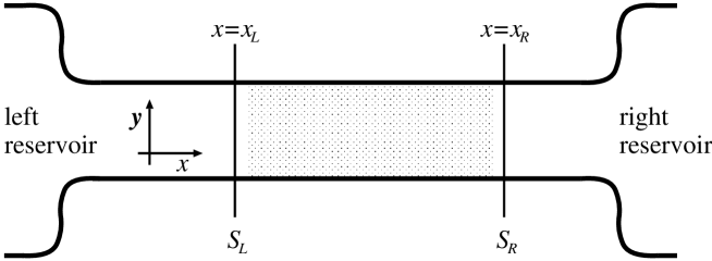
FIG. 1.: The conductor consists of a scattering region (dotted) connected by perfect leads to two electron reservoirs. Cross sections $S_{L}$ and $S_{R}$ in the left and right lead are indicated.

FIG. 2.: (a) The conductance (normalized by the Sharvin conductance $G_{S}=NG_{0}$) and (b) the shot-noise power (in units of $P_{\rm Poisson}\equiv 2e|\bar{I}|$), as a function of the ratio $L/\tilde{\ell}$, computed from Eqs. (34) and (36) for isotropic impurity scattering. The curves correspond to a three-dimensional (thin solid curve), two-dimensional (dashed curve), and a one-dimensional conductor (thick solid curve). The one-dimensional case is the analytical result from Eqs. (41) and (43). The two- and three-dimensional cases are numerical results.

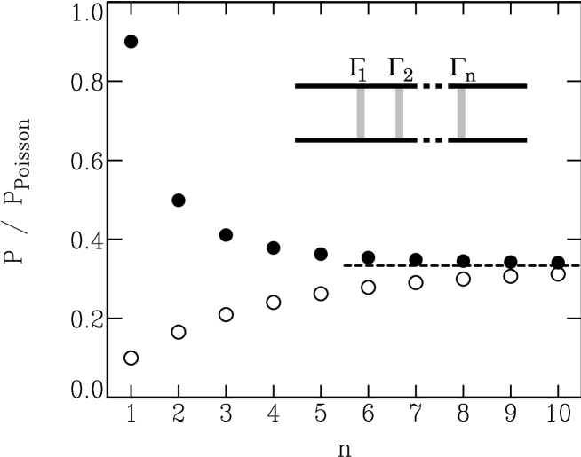
FIG. 3.: The shot-noise power $P$ for $n$ tunnel barriers in series with transmission probability $\Gamma=0.1$ (dots) and $\Gamma=0.9$ (circles), computed from Eq. (62). The dashed line is the large-$n$ limit $P=\frac{1}{3}P_{{\rm Poisson}}$. The inset shows schematically the geometry considered.

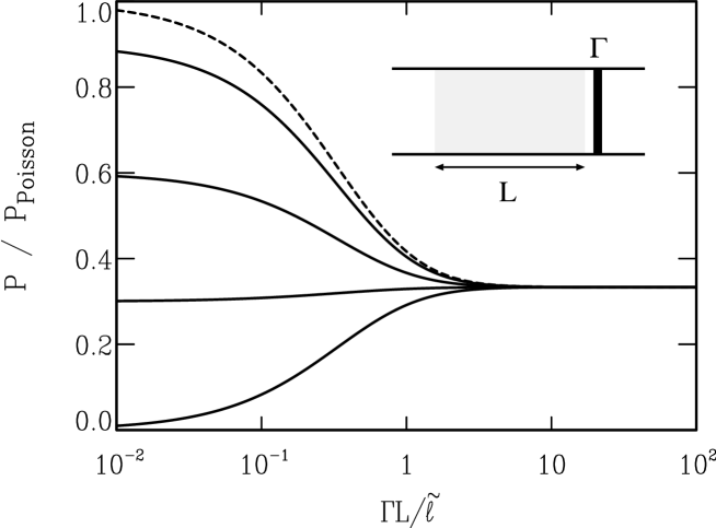
FIG. 4.: The shot-noise power $P$ for a conductor consisting of a disordered region in series with a planar tunnel barrier (see inset) as a function of its length $L$ (in units of $\tilde{\ell}/\Gamma$), for barrier transparencies $\Gamma=$1, 0.7, 0.4, and 0.1 (bottom to top). The dashed line is the limiting curve for $\Gamma\ll 1$. The curves are computed from Eq. (74) for a model with a one-dimensional density of states. The dimensionality dependence is expected to be small, compare Fig. 2.

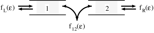
FIG. 5.: Both ends of the conductor are connected to an electron reservoir. Additional scattering inside the conductor is modeled by dividing it in two parts and connecting them through another reservoir. The electron distributions in the left and the right reservoir, $f_{L}(\varepsilon)$ and $f_{R}(\varepsilon)$, are Fermi-Dirac distributions. The distribution $f_{12}(\varepsilon)$ in the intermediate reservoir depends on the type of scattering.

FIG. 6.: The noise power $P$ (divided by the Johnson-Nyquist noise $4k_{B}T_{0}G$) versus applied voltage $V$ for a disordered wire for model (a) of quasi-elastic scattering (solid curve), (b) of electron heating (dashed curve), (c) of inelastic scattering (dash-dotted curve), according to Eqs. (108), (120), and (123), respectively. The upper left inset gives the electron distribution in the middle of the wire $f(\varepsilon,L/2)$ as a function of energy $\varepsilon$ for model (a), (b), and (c). The lower right inset shows the temperature $T_{e}(x)$ as a function of the position $x$ for model (b). For both insets, $k_{B}T_{0}=\frac{1}{20}e|V|$.

FIG. 7.: The noise power $P$ (divided by the Johnson-Nyquist noise $4k_{B}T_{0}G$) versus applied voltage $V$ for a disordered wire (bottom to top) in the ballistic limit $L/\tilde{\ell}\rightarrow 0$, the intermediate regime $L/\tilde{\ell}=1$, and in the diffusive limit $L/\tilde{\ell}\rightarrow\infty$, as given by Eq. (A19). The dashed line is the noise in a tunnel barrier, according to Eq. (A20).

REFERENCES

- [1] V. A. Khlus, Zh. Eksp. Teor. Fiz. 93 (1987) 2179 [Sov. Phys. JETP 66 (1987) 1243].
- [2] G. B. Lesovik, Pis’ma Zh. Eksp. Teor. Fiz. 49 (1989) 513 [JETP Lett. 49 (1989) 592].
- [3] B. Yurke and G. P. Kochanski, Phys. Rev. B 41 (1990) 8184.
- [4] M. Büttiker, Phys. Rev. Lett. 65 (1990) 2901; Phys. Rev. B 46 (1992) 12485.
- [5] Th. Martin and R. Landauer, Phys. Rev. B45 (1992) 1742.
- [6] C. W. J. Beenakker and M. Büttiker, Phys. Rev. B 46 (1992) 1889.
- [7] K. E. Nagaev, Phys. Lett. A 169 (1992) 103.
- [8] M. J. M. de Jong and C. W. J. Beenakker, Phys. Rev. B 46 (1992) 13400.
- [9] Yu. V. Nazarov, Phys. Rev. Lett.73 (1994) 134.
- [10] B. L. Altshuler, L. S. Levitov, and A. Yu. Yakovets, Pis’ma Zh. Eksp. Teor. Fiz. 59 (1994) 821 [JETP Lett. 59 (1994) 857].
- [11] F. Liefrink, J. I. Dijkhuis, M. J. M. de Jong, L. W. Molenkamp, and H. van Houten, Phys. Rev. B49 (1994) 14066.
- [12] O. N. Dorokhov, Solid State Commun. 51 (1984) 381; Y. Imry, Europhys. Lett. 1 (1986) 249; J. B. Pendry, A. MacKinnon, and P. J. Roberts, Proc. R. Soc. London Ser. A 437 (1992) 67.
- [13] A. Shimizu and M. Ueda, Phys. Rev. Lett.69 (1992) 1403.
- [14] R. Landauer (preprint).
- [15] M. J. M. de Jong, Phys. Rev. B49 (1994) 7778.
- [16] B. B. Kadomtsev, Zh. Eksp. Teor. Fiz. 32 (1957) 943 [Sov. Phys. JETP 5 (1957) 771].
- [17] Sh. M. Kogan and A. Ya. Shul’man, Zh. Eksp. Teor. Fiz. 56 (1969) 862 [Sov. Phys. JETP 29 (1969) 467].
- [18] I. O. Kulik and A. N. Omel’yanchuk, Fiz. Nizk. Temp. 10 (1984) 305 [Sov. J. Low Temp. Phys. 10 (1984) 158].
- [19] C. W. J. Beenakker and H. van Houten, Phys. Rev. B 43 (1991) 12066. The results presented in this paper are incorrect, because the equal-time correlation (Eq. (6) of Ref. [19]) is not generally valid.
- [20] M. J. M. de Jong and C. W. J. Beenakker, Phys. Rev. B51 (1995) 16867.
- [21] L. Y. Chen and C. S. Ting, Phys. Rev. B43 (1991) 4534.
- [22] J. H. Davies, P. Hyldgaard, S. Hershfield, and J. W. Wilkins, Phys. Rev. B46 (1992) 9620.
- [23] L. S. Levitov and G. B. Lesovik, Pis’ma Zh. Eksp. Teor. Fiz. 58, 225 (1993) [JETP Lett. 58 (1993) 230].
- [24] H. Lee, L. S. Levitov, and A. Yu. Yakovets, Phys. Rev. B51 (1995) 4079.
- [25] Y. P. Li, D. C. Tsui, J. J. Heremans, J. A. Simmons, and G. W. Weimann, Appl. Phys. Lett. 57 (1990) 774.
- [26] M. Reznikov, M. Heiblum, H. Shtrikman, and D. Mahalu, Phys. Rev. Lett.76 (1995) 3340.
- [27] A. Kumar, L. Saminadayar, D. C. Glattli, Y. Jin, and B. Etienne (preprint).
- [28] M. J. M. de Jong and C. W. J. Beenakker, in Coulomb and Interference Effects in Small Electronic Structures, edited by D. C. Glattli, M. Sanquer, and J. Trân Thanh Vân (Editions Frontières, France, 1994).
- [29] R. Landauer, Ann. N. Y. Acad. Sc. 755 (1995) 417.
- [30] S. V. Gantsevich, V. L. Gurevich, and R. Katilius, Rivista Nuovo Cimento 2 (5) (1979) 1.
- [31] O. M. Bulashenko and V. A. Kochelap, J. Phys. Condens. Matter 5 (1993) L469.
- [32] C. W. J. Beenakker and H. van Houten, Phys. Rev. Lett. 63 (1989) 1857.
- [33] Yu. V. Sharvin, Zh. Eksp. Teor. Fiz. 48 (1965) 984 [Sov. Phys. JETP 21 (1965) 655].
- [34] For a study of shot noise in one-dimensional conductors, see: V. I. Melnikov, Phys. Lett. A 198 (1995) 459.
- [35] R. C. Liu, P. Eastman, and Y. Yamamoto (preprint).
- [36] O. N. Dorokhov, Pis’ma Zh. Eksp. Teor. Fiz. 36 (1982) 259 [JETP Lett. 36 (1982) 318]; P. A. Mello, P. Pereyra, and N. Kumar, Ann. Phys. (N. Y.) 181 (1988) 290.
- [37] Y. P. Li, A. Zaslavsky, D. C. Tsui, M. Santos, and M. Shayegan, Phys. Rev. B41 (1990) 8388.
- [38] H. C. Liu, J. Li, G. C. Aers, C. R. Leavens, M. Buchanan, and Z. R. Wasilewski, Phys. Rev. B51 (1995) 5116.
- [39] S. Hershfield, J. H. Davies, P. Hyldgaard, C. J. Stanton, and J. W. Wilkins, Phys. Rev. B47 (1992) 1967; A. Levy Yeyati, F. Flores, and E. V. Anda, ibid. 47 (1993) 10543; K.-M. Hung and G. Y. Wu, ibid. 48 (1993) 14687; U. Hanke, Yu. M. Galperin, K. A. Chao, and N. Zou, ibid. 48 (1993) 17209; U. Hanke, Yu. M. Galperin, and K. A. Chao, ibid. 50 (1994) 1595.
- [40] J. A. Melsen and C. W. J. Beenakker, Physica B 203 (1994) 219.
- [41] C. W. J. Beenakker, B. Rejaei, and J. A. Melsen, Phys. Rev. Lett.72 (1994) 2470.
- [42] K. E. Nagaev, Phys. Rev. B52 (1995) 4740.
- [43] V. I. Kozub and A. M. Rudin, Phys. Rev. B52 (1995) 7853.
- [44] B. L. Altshuler, A. G. Aronov, and D. E. Khmelnitskii, J. Phys. C 15 (1982) 7367; A. Stern, Y. Aharonov, and Y. Imry, Phys. Rev. B41 (1990) 3436.
- [45] M. Büttiker, Phys. Rev. B38 (1988) 9375.
- [46] M. Büttiker, in Noise in Physical Systems and 1/f Fluctuations, edited by V. Bareikis and R. Katilius (World Scientific, Singapore, 1995).
- [47] J. H. Davies, J. Carlos Egues, and J. W. Wilkins, Phys. Rev. B52 (1995) 11259; see also: J. Carlos Egues, S. Hershfield, and J. W. Wilkins, ibid. 49 (1994) 13517.
- [48] See, e.g., H. van Houten, L. W. Molenkamp, C. W. J. Beenakker, and C. T. Foxon, Semicond. Sci. Technol. 7 (1992) B215.
- [49] J. M. Martinis and M. H. Devoret (unpublished).
- [50] A. Steinbach, J. M. Martinis, and M. H. Devoret, Bull. Am. Phys. Soc. 40 (1995) 400.
- [51] R. Landauer, Phys. Rev. B47 (1993) 16427.
- [52] R. C. Liu and Y. Yamamoto, Phys. Rev. B49 (1994) 10520; 50 (1994) 17411.
- [53] A. N. Korotkov, D. V. Averin, K. K. Likharev, and S. A. Vasenko, in Single-Electron Tunneling and Mesoscopic Devices, edited by H. Koch and H. Lübbig (Springer, Berlin, 1992); A. N. Korotkov, Phys. Rev. B49 (1994) 10381.
- [54] H. Birk, M. J. M. de Jong, and C. Schönenberger, Phys. Rev. Lett.75 (1995) 1610.
- [55] M. Büttiker, in Noise in Physical Systems and 1/f Fluctuations, edited by P. H. Handel and A. L. Chung (AIP, New York, 1993).