Directed polymers in high dimensions

Abstract

We study directed polymers subject to a quenched random potential in $d$ transversal dimensions. This system is closely related to the Kardar–Parisi–Zhang equation of nonlinear stochastic growth. By a careful analysis of the perturbation theory we show that physical quantities develop singular behavior for $d\to 4$. For example, the universal finite size amplitude of the free energy at the roughening transition is proportional to $\sqrt{4-d}$. This shows that the dimension $d=4$ plays a special role for this system and points towards $d=4$ as the upper critical dimension of the Kardar–Parisi–Zhang problem.

I Introduction

The field of non-equilibrium growth processes has attracted quite a lot of interest in the recent past [1]. The simplest nonlinear model describes a growing surface on sufficiently large length scales as a height profile $h(r,t)$ over a $d$–dimensional reference plane parameterized by $r$. The dynamics of this surface is given by the Kardar–Parisi–Zhang [2] (KPZ) equation

$${\partial\over\partial t}h=\nu\Delta h+\frac{1}{2}\lambda(\nabla h)^{2}+\eta$$ (1)

with a Gaussian white noise defined by

$$\overline{\eta(r,t)}=0\mbox{ and }\overline{\eta(r,t)\eta(r^{\prime},t^{\prime})}=\sigma^{2}\delta^{d}(r-r^{\prime})\delta(t-t^{\prime}).$$ (2)

The surface described by (1) can be in different phases which depend on the dimension-less coupling constant

$$g=-{\lambda^{2}\sigma^{2}\over 2\nu^{3}}.$$ (3)

and the space dimension $d$. In less than two dimensions there are two different phases: the weak coupling phase for $g=0$ and the strong coupling phase for $g\not=0$. Above two dimensions, there exists a critical value $g_{c}$. The surface is in the weak coupling phase for $|g|<g_{c}$ and in the strong coupling phase for $|g|>g_{c}$. Precisely at $|g|=g_{c}$ the system undergoes a roughening transition. Whereas the linear growth equation for $g=0$ can easily be solved in any dimension, it is much more difficult to get information on the critical behavior of the other phases.

The morphology of the surface in the different phases is characterized by the asymptotic scaling of the height-correlation-function

$\displaystyle\langle(h(r_{1},t_{1})-h(r_{2},t_{2}))^{2}\rangle\sim|r_{1}-r_{2}|^{2\chi}f(t|r_{1}-r_{2}|^{-z}),$which defines the roughening exponent $\chi$ and the dynamic exponent $z$. For $g\not=0$ these exponents satisfy the hyperscaling relation $z+\chi=2$ [3].

In the strong coupling phase it is known that $z=3/2$ in $d=1$ [4] and $z=2$ in the limit of infinite dimension [5]. In general dimensions all exact methods fail and only numerical and mode–coupling results are available, but they become less reliable in higher dimensions. Therefore there is still a very controversial discussion [6, 7, 8, 9, 10] about the existence of a finite upper critical dimension of the KPZ problem, i.e. a dimension above which the dynamical exponent $z$ has the constant value $2$.

In the language of the renormalization group, the different phases belong to different fixed points. For less than two dimensions, there is one unstable fixed point at $g=0$, which governs the weak coupling phase, and one stable fixed point at $g\to-\infty$, which governs the strong coupling phase. Above two dimensions, the weak coupling fixed point also becomes stable and a new fixed point describing the roughening transition appears in between the other fixed points.

It has been shown [11] that the strong–coupling fixed point is inaccessible by a perturbation expansion around $g=0$. The situation is somewhat better for the fixed point describing the roughening transition. The singularities, which arise in the perturbation series above two dimensions, can be treated in a systematic expansion [12, 13] with parameter

$$\epsilon={2-d\over 2}.$$ (4)

In the framework of this $\epsilon$-expansion, one finds the exponents $z^{*}=2$ and $\chi^{*}=0$, which are exact to all orders in perturbation theory [11]. Hence, hyperscaling is preserved.

However, this perturbation expansion breaks down for $d\to 4$ since new singularities in the coefficients of the series expansions arise at $\epsilon^{\prime}=0$, where

$$\epsilon^{\prime}\equiv\epsilon+1={4-d\over 2}.$$ (5)

The treatment of these singularities is the aim of this paper. We develop a systematic way to extract the behavior of physical quantities as $d\to 4$ from the divergent series in $\epsilon^{\prime}$. We show that in contrast to the singularities in $\epsilon$, these singularities translate into a non-analytic behavior of observable quantities. This stresses the importance of $d=4$ for the KPZ problem and therefore shows that four dimensions is a good candidate for an upper critical dimension.

We will address this question not in the KPZ picture but by using the exact Hopf–Cole–mapping [14, 15] of the KPZ problem to a directed polymer in a random medium. A directed polymer (also called a string) is a line with a preferred direction, which is governed by its line tension. The energy of a given conformation is

$${\cal H}[r]=\int_{0}^{L_{||}}\frac{1}{2}\dot{r}^{2}(t)+\lambda\nu^{-3/2}\eta(r(t),t){\rm d}t,$$ (6)

where $r(t)$ is a $d$-dimensional vector which denotes the elongation of the directed polymer at a position along the preferred (“time”) axis $t$, $L_{||}$ is the projected length of the directed polymer and $\eta$ is the random potential which appears in the KPZ equation.

To study the structure of the new singularities in the perturbation series, we will use an especially simple physical quantity. We nevertheless expect, that more complicated quantities such as correlation functions show the same type of singularities. We will study a system where the projected length $L_{||}$ of the directed polymer is infinite while its transversal “motion” is restricted to a finite volume of a characteristic width $L_{\perp}\equiv L^{1/2}$. Within this system we will concentrate on the dimension-less averaged free energy per unit “time”, which we call

$${\cal C}(g,L)=\lim_{L_{||}\to\infty}{L\over L_{||}}\overline{F(g,L,L_{||})}.$$ (7)

The infrared regularization by the length scale $L$ has to be introduced, because the series expansion starts at the Gaussian fixed point ($g=0$), which has no intrinsic length scale. $L$ moreover serves as the flow parameter of the renormalization group considered below.

Since at the roughening transition hyperscaling is preserved at least around $2$ dimensions [11], therefore there are no corrections to the $1/L_{\perp}^{2}=1/L$ behavior of the free energy per length $\overline{F(g,L,L_{||})}/L_{||}$, and the finite size amplitude

$${\cal C}(g)=\lim_{L\to\infty}{\cal C}(g,L)$$ (8)

is a universal quantity. Near $d=2$, one finds [11] for its value ${\cal C}^{*}$ at the unbinding transition

$${\cal C}^{*}(\epsilon)\sim\epsilon+O(\epsilon^{2}).$$ (9)

$\cal C$ is not only one of the simplest physical quantities to be calculated in our system, but also one of the most fundamental ones: it plays a role very similar to the central charge in two-dimensional conformal models [17].

The directed polymer problem with randomness described by (6) can be treated analytically via the replica trick. This means that it can be expressed as the limiting case $N\to 0$ of $N$ directed polymers with a short-ranged interaction potential (see e.g. [16]):

$\displaystyle{\cal H}[r_{1},\ldots,r_{N}]=\int_{0}^{L_{||}}\frac{1}{2}\sum_{i=1}^{N}\dot{r}_{i}^{2}(t)+g\sum_{i<j}^{N}\delta(r_{i}(t)-r_{j}(t)){\rm d}t.$By (3), the potential is always attractive ($g<0$) and captures the short–ranged correlations of the disorder (2).

The finite size amplitude (7) of the free energy per unit “time” of the random system can then be obtained from the limit $N\to 0$ of the finite size amplitudes per unit “time” and per pair of directed polymers

$${\cal C}(g,L,N) = {2\over N(N-1)}$$

$$\times\!\lim_{L_{||}\to\infty}{L\over L_{||}}[F(g,L,N,L_{||})-\!F(0,L,N,L_{||})]$$

of the $N$-polymer system without randomness.

The development of a new regularization scheme for the perturbation theory of $\cal C$ near 4 dimensions is done in two steps. In the first step, the fact is used that for only two directed polymers independent techniques exist, that allow an exact solution of the 2–polymer–problem. Those methods (the transfer matrix approach and the resummation of the perturbation series) are reviewed and extended to our system with a transversally restricted “movement” in section II of this paper

In order to be able to get results about perturbation series where no exact solution exists any more, a regularization scheme is developed by comparison with the exact solution. The regularization scheme itself then is independent of the existence of the exact solution in the sense that it extracts the results directly from the coefficients of the new singularities in the perturbation series. It is shown that only the most divergent terms in every order of perturbation theory contribute to the first order terms of the limiting $\beta$ function.

As the second step this regularization scheme is then applied to the case of an arbitrary number of directed polymers in section III, which can only be solved exactly in one dimension [18]. A diagrammatic expansion of the partition function and of the free energy is developed. The series expansion is calculated up to the fifth order in the coupling constant and many simplifications appear, that suggest a simple underlying structure.

Since the most important diagrams with respect to the regularization scheme turn out to be just 2-polymer-diagrams, the main properties of the $\beta$ function can still be extracted from the general structure of the perturbation series.

Independent of the number of directed polymers in less then 4 dimensions there are two zeroes of the $\beta$ function: one is the finite size amplitude ${\cal C}^{*}$ of the free energy per unit “time” at the unbinding transition; the other one is at the Gaussian fixed point. In 4 dimensions the $\beta$ function becomes just a straight line with a fixed slope. ${\cal C}^{*}$ and the zero at the Gaussian fixed point coincide there. We find that near 4 dimensions the physical quantity ${\cal C}^{*}$ behaves non–analytically as

$${\cal C}^{*}(\epsilon^{\prime})\sim\sqrt{\epsilon^{\prime}}.$$ (10)

Since the behavior is independent of the number of directed polymers, it should also describe the scenario in the replica limit of a vanishing number of directed polymers and therefore the behavior of the weak-coupling fixed point of the KPZ problem.

In section IV, the main results are summarized again. Many of the technical details have been postponed to various appendices to keep the route of argumentation straight.

II Two directed polymers

Since the problem of two directed polymers ($N=2$) is especially simple, we start examining this problem and try to generalize our results in the next section.

The reason for the simplicity of the two polymer problem is that one can separate the problem in the motion of a “center of mass” $({\bf r}_{1}(t)+{\bf r}_{2}(t))/2$, which just fluctuates freely independent of the coupling constant $g$ and the problem in the relative coordinate $\hat{r}\equiv{\bf r}_{2}-{\bf r}_{1}$. Since the KPZ–problem is equivalent to directed polymers with a relative short–range interaction ($V(r_{1},r_{2})=g\delta^{d}(r_{1}-r_{2})$), we have to deal in the relative coordinate with one directed polymer, which is interacting with a straight line defect at the origin of the perpendicular space. The transition probability from ${\bf r}^{\prime}$ to ${\bf r}$ within the projected contour length $t$ (the restricted partition function) is given by the single path integral

$$Z_{t}({\bf r}^{\prime},{\bf r})=\int_{(0,{\bf r}^{\prime})}^{(t,{\bf r})}{\cal D}\hat{r}\exp\left[-\int_{0}^{t}\frac{1}{2}\dot{\hat{r}}^{2}(t^{\prime})+V(\hat{r}(t^{\prime})){\rm d}t^{\prime}\right].$$ (11)

The problem of one directed polymer interacting with a defect line can now be treated in different manners: On the one hand the path integral formulation of the directed polymer problem is equivalent to a “quantum mechanics” and can be solved in analogy to the corresponding quantum mechanical problem. This is called the transfer matrix approach because the Hamiltonian of the quantum mechanics is the continuum transfer matrix of the problem.

The second approach just sets up a perturbative expansion of the problem with the defect with the strength of the defect as the expansion parameter, which can either be calculated coefficient by coefficient or in the special case of two directed polymers can even be summed up completely.

A comparison of these approaches shows that they lead to the same results. Because we know the exact solutions, we can use them to develop a treatment of the perturbation series in the interesting case $\epsilon^{\prime}\to 0$, which we afterwards can apply to problems where no exact solution is available any more, as for example the case of more than two directed polymers.

A Transfer matrix results

Since the path integral (11) is formally a quantum mechanical path integral in imaginary time, the partition function obeys the Schroedinger equation

$$(-\Delta+V({\bf r}))Z_{t}({\bf r}^{\prime},{\bf r})=-{\partial\over\partial t}Z_{t}({\bf r}^{\prime},{\bf r}),$$ (12)

of a particle in a potential $V({\bf r})$, which can be attacked by standard quantum mechanical methods.

If the movement is restricted to a finite volume characterized by some length $L_{\perp}=L^{\frac{1}{2}}$, the long–time (large projected length of the directed polymer) behavior of the partition function is an exponential decay, the decay rate of which is given by the ground state energy of the quantum mechanical problem

$$(-\Delta+V({\bf r}))\psi({\bf r})=E_{0}\psi({\bf r}),$$ (13)

The free energy per unit “time” for long polymers is therefore given by the ground state energy plus exponentially small corrections. The finite size coefficient can be extracted by studying the behavior of the free energy for large system sizes $L_{\perp}$. At the Gaussian fixed point we expect from dimensional analysis that $E_{0}\sim\frac{1}{L_{\perp}^{2}}=\frac{1}{L}$. The prefactor of this decay is ${\cal C}$. In order to calculate ${\cal C}$, we extend here the calculations in [19] to the case of “movement” in a finite volume.

1 Precise definition of the model

In order to solve the model in arbitrary dimensions, we have to use potentials and boundary conditions, which have a spherical symmetry. In this case, we can separate the wave function in a radial and an angular part. As it is well known from quantum mechanics, it is convenient to define the radial function $\Phi(r)$ to be $r^{(d-1)/2}$ times the radial part of the total wave function. This function obeys for the lowest (zero) angular momentum - as it should be the case for the ground state - the radial Schroedinger equation

$$-{\partial^{2}\over\partial r^{2}}\Phi(r)+\!{(d-3)(d-1)\over 4}{1\over r^{2}}\Phi(r)+\!V(r)\Phi(r)\!=\!\tilde{E}_{0}\Phi(r).$$ (14)

We implement the attractive potential at the origin as a well potential with a small but finite extension $a$:

$$V(r)=\left\{\begin{array}[]{rl}-\tilde{V}_{0}&0\leq r<a\\ 0&a\leq r\end{array}\right.$$ (15)

By defining $\phi(r)\equiv\Phi(ra)$, $E_{0}\equiv a^{2}\tilde{E}_{0}$, $\bar{V}(r)\equiv a^{2}V(ra)$ and $V_{0}\equiv a^{2}\tilde{V}_{0}$, the ultraviolet cutoff $a$ can be eliminated and everything is written in dimension-less variables.

The boundary conditions imposed to the directed polymer have to be radially symmetric, too. The two possibilities studied here in detail are on the one hand the Dirichlet boundary conditions, where the directed polymer is put into a spherical box of radius $L_{\perp}$ with hard walls, which means $\phi(L_{\perp}/a)=0$, and on the other hand the von-Neumann boundary conditions, which impose that the first derivative of the radial part of the wave function vanishes at the boundary of a spherical box of radius $L_{\perp}$, in order to mimic a kind of periodic boundary conditions. This is equivalent to the condition

$${L\over a}\left.{\partial\over\partial y}\right|_{y={\frac{L_{\perp}}{a}}}\phi(y)={d-1\over 2}\phi(\frac{L_{\perp}}{a})$$ (16)

for the radial function $\phi$.

Moreover we will consider harmonic boundary conditions. That means that we allow a “movement” in infinite space, but add an harmonic well potential $(\gamma/2)r^{2}$, which effectively restricts the motion. The associated width of the box is from dimensional analysis $\sqrt{\gamma}=(\pi/2)(1/L_{\perp}^{2})$. (The factor of $\pi/2$ has only been introduced for convenience).

2 Results for the free energy

For the potential as given by 15 and the first two boundary conditions given in the above section, it is relatively easy, to calculate the ground state energy, because the potential is piecewise constant. Only standard techniques of quantum mechanics are applied. A sketch of these calculations is given in appendix A.

Here, we just give the results for the ground state energy. Let us first consider the Dirichlet boundary conditions.

For the free system ($V_{0}=0$) the ground state energy is exactly given by

$$E_{0}=x_{|\epsilon|}^{2}\left(\frac{a}{L_{\perp}}\right)^{2},$$ (17)

with $x_{|\epsilon|}$ being the smallest positive root of the Bessel function $J_{|\epsilon|}$. This is also the asymptotic behavior for $0<V_{0}<V_{*}$. At the phase transition point ($V_{0}=V_{*}$) we have

$$E_{0}\approx\left\{\begin{array}[]{ll}y_{|\epsilon|}^{2}\left(\frac{a}{L_{\perp}}\right)^{2}&|\epsilon|<1\\ 4(|\epsilon|-1)\left(\frac{a}{L_{\perp}}\right)^{2|\epsilon|}&|\epsilon|>1\end{array}\right.$$ (18)

where $y_{|\epsilon|}$ is the smallest positive root of $J_{-|\epsilon|}$.

For von-Neumann boundary conditions the ground state energy is zero at $V_{0}=0$. At $0<V_{0}<V_{*}$ the asymptotic behavior is

$$E_{0}\approx-{4|\epsilon|(|\epsilon|+1)\over 2|\epsilon|{J_{|\epsilon|}(\sqrt{V_{0}})\over\sqrt{V_{0}}J_{|\epsilon|+1}(\sqrt{V_{0}})}-1}\left(\frac{a}{L_{\perp}}\right)^{2(|\epsilon|+1)}.$$ (19)

The decay is faster than quadratic which means that the coefficient we are looking for remains zero. This scaling behavior of the free energy per length in a system of finite transversal size at the unbinding transition is consistent with the scaling behavior of the eigenenergy of the bound state in the infinite system [20].

At the phase transition we get

$$E_{0}\approx\left\{\begin{array}[]{ll}-z_{|\epsilon|}^{2}\left(\frac{a}{L_{\perp}}\right)^{2}&|\epsilon|<1\\ 4\sqrt{|\epsilon|(|\epsilon|^{2}-1)}\left(\frac{a}{L_{\perp}}\right)^{|\epsilon|+1}&|\epsilon|>1\end{array}\right.$$ (20)

where $z_{|\epsilon|}$ is the smallest positive root of $I_{-|\epsilon|-1}$. The decay for $|\epsilon|>1$ is again faster than quadratic.

The differences between the decay coefficients at the phase transition point and in the free case (which we defined to be ${\cal C}^{*}$ in the introduction) are plotted against the dimension in Fig. 1.

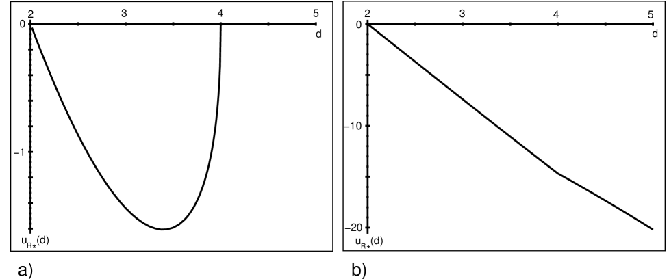
FIG. 1.: Transfer matrix results for the renormalized coupling constant. The dependence on the dimensionality is shown for von-Neumann (a) and Dirichlet (b) boundary conditions.

It can be seen that ${\cal C}^{*}$ stays finite as $d$ approaches 4 with Dirichlet boundary conditions, whereas for von-Neumann boundary conditions ${\cal C}^{*}$ approaches zero. From the first three terms of the series expansion of the Bessel function $I_{-|\epsilon|-1}$ (the third term is the first one with a non-vanishing coefficient in the limit $|\epsilon|\to 1$) we get near $|\epsilon|=1$ a behavior of $z_{|\epsilon|}\sim 4\sqrt{(1+|\epsilon|)(1-|\epsilon|)}+4(|\epsilon|-1)$, which yields equation (10).

For harmonic boundary conditions the differential equation in the outer area is a bit more complicated. Its solution is

$$\Phi(y)\sim y^{-\frac{1}{2}}W_{{E_{0}\over 4\sqrt{\gamma}a^{2}},\frac{\epsilon}{2}}(\sqrt{\gamma}a^{2}y^{2})$$ (21)

with the Whittaker function $W_{\lambda,\mu}(z)$. The condition of differentiability at $y=1$ is also more complicated to evaluate than for the von-Neumann or Dirichlet boundary conditions, but in the end we get

$$E_{0}\sim\pi\frac{d}{2}\left(a\over L_{\perp}\right)^{2}$$ (22)

at $0<V_{0}<V_{*}$ and

$$E_{0}\sim\pi\left(2-\frac{d}{2}\right)\left(a\over L_{\perp}\right)^{2}$$ (23)

at the phase transition $V_{0}=V_{*}$. Therefore

$${\cal C}=\pi(2-d)=2\pi\epsilon.$$ (24)

B General perturbation theory

Starting from the partition

$${\cal H}={\cal H}_{0}+g\int_{0}^{L_{||}}\Phi(t){\rm d}t\quad\mbox{with}\quad\Phi(t)\equiv\delta^{d}(r(t))$$ (25)

into the free part (kinetic part and infrared regularization) and an interaction part we can easily set up a perturbation series of the partition function as

$${Z\over Z_{0}} = \langle e^{-g\int_{0}^{L_{||}}\Phi(t){\rm d}t}\rangle_{0}$$ (26)

$$= 1+\sum_{n=1}^{\infty}(-g)^{n}\int\limits_{\hbox to0.0pt{\hbox{$\hskip 19.91692pt\scriptstyle 0\leq t_{1}\leq\ldots\leq t_{n}\leq L_{||}$}\hss}}{\rm d}t_{1}\ldots\int{\rm d}t_{n}\langle\Phi(t_{1})\ldots\Phi(t_{n})\rangle_{0}$$ (27)

where the expectation values $\langle\ldots\rangle_{0}$ are taken with respect to ${\cal H}_{0}$ and $Z_{0}$ is the partition function just for ${\cal H}_{0}$. Here the factor of $n!$ has been canceled out by introducing a time ordering.

The free energy is the negative logarithm of the partition function and can also be expressed as a series in $g$ by systematically expanding the logarithm. Since all correlation functions are translationally invariant in the limit of large $L_{||}$, one of the integrations just gives a factor of $L_{||}$ which cancels out since we are interested in the free energy per length. As a result of this series expansion we get to the first orders

$$\lim\limits_{L_{||}\to\infty}{F(g)-F(0)\over L_{||}}=$$

$$g\langle\Phi(0)\rangle_{0}-g^{2}\int_{0}^{\infty}\langle\Phi(0)\Phi(t)\rangle_{0}-\langle\Phi(0)\rangle_{0}^{2}{\rm d}t+O(g^{3}).$$

Since the structure of the singularities in the case $d\to 4$ does not show up in the second order, we have to extend the perturbation series to higher orders. (Higher terms of this formula can be found in appendix B.)

For two directed polymers with a $\delta$ interaction it is now particularly simple to calculate the time ordered correlation functions, because they can be reduced to two-point-functions. Consider the propagator $G_{t}(r_{1},r_{2})$ of the relative coordinate of the free (only infrared regularized) directed polymers. With this, the multi-point-function is expressed as

$$\langle\Phi(t_{1})\ldots\Phi(t_{n})\rangle_{0}={\int{\rm d}r_{1}\int{\rm d}r_{2}G_{t_{1}}(r_{1},0)G_{t_{2}-t_{1}}(0,0)\ldots G_{t_{n}-t_{n-1}}(0,0)G_{L_{||}-t_{n}}(0,r_{2})\over\int{\rm d}r_{1}\int{\rm d}r_{2}G_{L_{||}}(r_{1},r_{2})}.$$ (28)

For long chain length we can drop end effects and assume $t_{1}$ and $L_{||}-t_{n}$ to be large enough so that we can combine those terms to a one point function

$$\langle\Phi(t_{1})\ldots\Phi(t_{n})\rangle_{0}\!=G_{t_{2}-t_{1}}(0,0)\ldots G_{t_{n}-t_{n-1}}(0,0)\langle\Phi(0)\rangle_{0}$$ (29)

If we here set $n=2$ we get the relation between the return probability $G_{t}(0,0)$ and the two point function, so that we can express the multi-point function by two point functions as

$$\langle\Phi(t_{1})\ldots\Phi(t_{n})\rangle_{0} = {1\over\langle\Phi(0)\rangle_{0}^{n-2}}$$

$$\times\langle\Phi(t_{1})\Phi(t_{2})\rangle_{0}\ldots\langle\Phi(t_{n-1})\Phi(t_{n})\rangle_{0}.$$

Using this formula, we can express all the coefficients of the perturbation series as multiple integrals over products of two-point functions. It is even more convenient to introduce the dimension-less connected two point function as

$\displaystyle g_{1}(s)\equiv{\langle\Phi(0)\Phi(Ls)\rangle_{0,c}\over\langle\Phi(0)\rangle_{0}^{2}}\equiv{\langle\Phi(0)\Phi(Ls)\rangle_{0}-\langle\Phi(0)\rangle_{0}^{2}\over\langle\Phi(0)\rangle_{0}^{2}}.$If we now introduce a dimension-less coupling constant

$$u_{0}\equiv gL^{\epsilon}=gL\langle\Phi(0)\rangle_{0},$$ (30)

the finite size coefficient of the free energy per unit “time” reads

$${\cal C}(u_{0}) = L\lim_{L_{||}\to\infty}{F(g)-F(0)\over L_{||}}=$$ (31)

$$= u_{0}-u_{0}^{2}\int_{0}^{\infty}g_{1}(s){\rm d}s$$ (34)

$$+u_{0}^{3}\int_{0}^{\infty}\!\int_{0}^{\infty}\!\Big{[}g_{1}(s_{1})g_{1}(s_{2})-g_{1}(s_{1}+s_{2})\Big{]}{\rm d}s_{1}{\rm d}s_{2}$$

$$+O(u_{0}^{4}),$$

where the time-ordered integration has been broken up into integrals over the respective time differences.

As we can see, the finite size coefficient is equal to the dimension-less coupling constant $u_{0}$ to first order. Singularities in this series can only arise in the integrals of the higher order terms. The renormalized coupling constant must be defined such that all singularities in the higher order terms are canceled. This is done by imposing the renormalization point condition for the renormalized coupling constant

$$u_{R}(u_{0})={\cal C}(u_{0}).$$ (35)

This renormalization point condition has the advantage, that it gives a physical meaning to the renormalized coupling constant.

Now we have to study the perturbation series (31) in detail. Already in the third order the essential difference between the regularization scheme at $\epsilon=0$ and at $\epsilon^{\prime}=0$ becomes obvious. Near $\epsilon=0$, the second term in the third order coefficient does not diverge at all, so that only the first term, which obviously factorizes to the square of the second order coefficient, produces divergences. This statement is true to all orders of perturbation theory, which produces just a geometric series of divergences. The especially simple structure of those divergences guarantees that the $\beta$ function calculated to the second order is exact to all orders of perturbation theory [11, 21].

Near $\epsilon^{\prime}=0$ the situation is totally different, because here also the second term diverges. So in every order combinations of different types of divergences occur, which do not factorize any more.

Since the terms in the perturbation series are becoming quite nasty in higher orders, it is convenient to introduce a graphical representation. Therefore we will draw in the $n$-th order $n$ points in a line which represent the $n$ time stamps involved. For each function $g_{1}$ we then draw a line connecting the two time stamps which are the arguments of the two point function. With this representation we can sketch our series expansion up to higher orders as it is done in appendix B.

Careful inspection shows that all diagrams appear that have at least one line passing each interval between two points and do not have two lines leaving one point in the same direction. The corresponding prefactors up to the seventh order are given by

$$(-1)^{\#P-l-1}\prod_{p\in P}l_{p}!,$$ (36)

where $l$ is the number of lines in the diagram, $P$ is the set of points in the diagram and for each $p\in P$ $l_{p}$ denotes the number of lines which pass the given point.

This perturbation series can be further simplified by applying some relations among the integrals over two point functions as for example

Those relations can be produced by a general mechanism via Laplace transformation as explained in detail in appendix C.

Applying them consequently enables us to get rid of all “nested” diagrams. Since we are finally interested in the inverse series to this one, we can just invert it by standard techniques order by order and end up with the series expansion of $u_{0}(u_{R})$

We will further discuss the structure of this series in a later section.

C Resummed perturbation theory

For two directed polymers interacting by a short range interaction (or equivalently one directed polymer interacting with a straight defect line by a short range interaction), an exact implicit equation for the dependence of the free energy per length from the interaction constant can be given by resummation of the perturbation series.

In order to get these results, we review here the summation technique given in [22] and generalize it to arbitrary boundary conditions. After we got the implicit equation we will study some useful examples of specific boundary conditions.

1 Resummation for arbitrary boundary conditions

The main idea, which leads to the summability, is that the coefficients of the perturbation series of the partition function have a product structure, which leads to a simple geometric series if they are properly decoupled.

This decoupling is achieved by Laplace transforming the constituents of equation (28). We will call them for simplicity

$\displaystyle f(t)\equiv G_{t}(0,0),\quad{\cal N}\equiv\int{\rm d}r_{1}\int{\rm d}r_{2}G_{L_{||}}(r_{1},r_{2}),$

$\displaystyle g(t)\equiv\int{\rm d}rG_{t}(r,0),\quad\mbox{and}\quad h(t)\equiv\int{\rm d}rG_{t}(0,r).$Their Laplace transforms are denoted by $\hat{f}$, $\hat{g}$ and $\hat{h}$ respectively.

Performing the Laplace transformation on the coefficients of the partition function, an implicit equation for the free energy per length can be extracted. The argumentation is given in appendix D. The result is that

$$\lim_{L_{||}\to\infty}{F(g)\over L_{||}}=-z_{0}.$$ (37)

where $z_{0}$ is the solution of

$$1+g\hat{f}(z)=0$$ (38)

with the largest (absolutely smallest) real part.

This is an exact implicit equation for the free energy per length derived from perturbation theory.

Introducing again dimension-less coupling constants we get the equation

$$1+u_{0}L^{-\epsilon}\hat{f}(L^{-1}(-f_{0}-u_{R}))=0,$$ (39)

where $f_{0}$ denotes the dimension-less free energy per length of the free ($u_{0}=0$) problem. As it is obvious from the above equation, it can be calculated as the smallest pole of the function $\hat{f}(-L^{-1}z)$.

To further improve this equation, we write it as

$$1+u_{0}F(u_{R})=0$$ (40)

with $F(z)\equiv L^{-\epsilon}\hat{f}(L^{-1}(-f_{0}-z))$. Since this equation has to be fulfilled for $u_{0}=0$ and $u_{R}=0$, $F$ has to behave like $-1/z$ at zero (which can also be verified for specific infrared regularizations). This means that $H(z)\equiv F(z)+1/z$ is a regular function at zero. Expressed by $H$ instead of $F$, the implicit equation for $u_{0}(u_{R})$ reads

$$u_{R}-u_{0}+u_{0}u_{R}H(u_{R})=0$$ (41)

2 Results for specific infrared regularizations and the duality relation

Now we want to calculate $H$ for specific infrared regularizations, in order to compare the general equation (41) with results from the literature.

Therefore we first reconsider the definition of $H(z)$

$$H(z) = L^{\epsilon}\int_{0}^{\infty}G_{t}(0,0)e^{{f_{0}+z\over L}t}{\rm d}t+{1\over z}$$ (42)

$$= \int_{0}^{\infty}\left[L^{1-\epsilon}G_{sL}(0,0)e^{f_{0}s}-1\right]e^{zs}{\rm d}s$$ (43)

From dimensional analysis $G_{sL}(0,0)$ must have the form

$$G_{sL}(0,0)=(sL)^{\epsilon-1}g_{IR}(sL).$$ (44)

Since $G_{sL}(0,0)$ has to decay exponentially with the ground state energy of the quantum mechanical problem, i.e. like $e^{-sf_{0}}$, it is easy to see that $H(z)$ is well-defined for $z\to 0$ in the infrared, because it follows that

$$L^{(1-\epsilon)}G_{sL}(0,0)e^{f_{0}s}-1=s^{\epsilon-1}h_{IR}(s)$$ (45)

with a for large arguments exponentially decaying function $h_{IR}(z)$.

Also it is clear that ultraviolet divergences arise for $\epsilon\to 0$. The derivatives of $H$ with respect to $z$ are less divergent in the ultraviolet regime; the $k$-th derivative will develop ultraviolet divergences at $\epsilon\to-k$. Thus in the case $\epsilon^{\prime}\to 0$ which we are interested in, also the first derivative of $H$ at $z=0$ is ultraviolet divergent.

The easiest case is the harmonic regularization, because the full propagator of the quantum mechanical harmonic oscillator is analytically known in all dimensions [23]. From this we extract the return probability for our directed polymer problem by inserting ${\bf r}={\bf r}^{\prime}=0$ and get

$$L^{1-\epsilon}G_{sL}(0,0)=(2\sinh(\pi s))^{-(1-\epsilon)}$$ (46)

From the decay at large $s$ we conclude $f_{0}=\pi\frac{d}{2}$.

The Laplace transform of this function can be explicitly performed ([24] 3.541) and gives

$$F(z)={\Gamma(\epsilon)\over 2\pi}{\Gamma(-{z\over 2\pi})\over\Gamma(\epsilon-{z\over 2\pi})}$$ (47)

For $d=1$ or $\epsilon=\frac{1}{2}$ this formula together with the equation (40) coincides with the one–dimensional transfer matrix result in [25]. We want to stress that we just calculated the full transition function for the free energy from the Gaussian to the non–Gaussian fixed point in any dimension in the case of a harmonic boundary condition.

It is remarkable that for $d=3$ or $\epsilon=-1/2$ the equation (40) is equivalent to the $d=1$ case, if one replaces $g$ up to a numerical factor by $-1/g$. This shows a duality (which exists for all dimensions which are symmetric with respect to $d=2$): The transition from the Gaussian fixed point in a dimension below $d=2$ via an repulsive interaction to the non-Gaussian fixed point is exactly the same as the transition from the Gaussian fixed point in the symmetric dimension above $d=2$ to the non–Gaussian fixed point via an attractive potential.

An explicit calculation of the Laplace transform of the propagator with hard wall (Dirichlet) boundary conditions (see appendix E) in $d=3$ gives the equation

$$\frac{8}{u_{0}}=\sqrt{2(u_{R}+f_{0})}\cot(\sqrt{2(u_{R}+f_{0})})$$ (48)

which shows the same duality relation with the transfer matrix result for $d=1$ in [25].

D Comparison of the two perturbative approaches

We will now see that the resummed and the naive perturbation series after all manipulations presented in the last two sections are exactly equivalent.

The resummation method gives us the exact relation (41) between the finite size coefficient $u_{R}$ of the free energy per length and the dimension-less coupling constant $u_{0}$. If we assume that $H$ can be expanded in a Taylor series around $z=0$, a perturbation series can be easily extracted from this equation and it is the same perturbation series as we already calculated directly, if we identify

$\displaystyle a_{n}\equiv\underbrace{\begin{picture}(168.0,15.0)(56.0,796.0)\put(160.0,800.0){\circle*{8.0}} \put(200.0,800.0){\circle*{8.0}} \put(180.0,800.0){\circle*{8.0}} \put(220.0,800.0){\circle*{8.0}} \put(80.0,800.0){\circle*{8.0}} \put(140.0,800.0){\oval(160.0,20.0)[tr]} \put(140.0,800.0){\oval(160.0,20.0)[tl]} \put(120.0,800.0){\circle*{8.0}} \put(100.0,800.0){\circle*{8.0}} \put(60.0,800.0){\circle*{8.0}} \put(140.0,800.0){\circle*{8.0}} \end{picture}}_{\hbox{$n$ intervals}}\equiv{1\over(n-1)!}\left.{{\rm d}^{n-1}\over{\rm d}z^{n-1}}\right|_{0}H(z).$Using the specific representation (42) of $H(z)$ by the function $h_{IR}(z)$ (45), which is directly connected to the return probability of the free problem, the coefficients are calculated as

$$a_{n}={1\over(n-1)!}\int_{0}^{\infty}s^{\epsilon-1+n-1}h_{IR}(s){\rm d}s$$ (49)

For the comparison with the transfer matrix results, we have to calculate the free energy per length at the transition point. Because we did use a renormalization point condition, which gives the renormalized coupling constant a physical meaning, in this framework, the finite size coefficient of the free energy per length is just the fixed point value of the renormalized coupling constant.

This fixed point value is the root of the $\beta$ function, which describes the flux of the renormalized coupling constant, and which according to the chain rule is given by

$$\beta(u_{R})=\epsilon{u_{0}(u_{R})\over{\partial\over\partial u_{R}}u_{0}(u_{R})}.$$ (50)

Using equation (40) this can be expressed as

$$\beta(u_{R})=-\epsilon{F(u_{R})\over F^{\prime}(u_{R})}.$$ (51)

This enables us to calculate this $\beta$-function explicitly in the case of a harmonic infrared regularization, where the Laplace transform of the return probability can be performed (47). The result is

$$\beta(u_{R})={2\pi\epsilon\over\Psi(-{u_{R}\over 2\pi})-\Psi(\epsilon-{u_{R}\over 2\pi})}$$ (52)

with the digamma function $\Psi(z)={{\rm d}\over{\rm d}z}\ln\Gamma(z)$. The behavior of the $\beta$ function already has been shown in Fig. 2. For $\epsilon<0$ there is always one negative root and the slope of the $\beta$ function at the root is $-\epsilon$. It is remarkable that the $\beta$ function has a well defined limit function for $\epsilon\to-1$ ($\epsilon^{\prime}\to 0$), which is the case we are mostly interested in. The limiting $\beta$ function is just the straight line $u_{R}+2\pi$.

FIG. 2.: The $\beta$ function of a directed polymer in a harmonic potential.

E The limit $\epsilon^{\prime}\to 0$

In the last section, we remarked that despite of the singularities in the coefficients of the perturbation series, a limiting $\beta$ function for $\epsilon^{\prime}\to 0$ exists. We heavily used the fact that we could calculate a closed form expression for the $\beta$ function, and its properties are a bit awkward. Especially $\beta(0)$ is not zero any more in contrary to all finite orders of perturbation theory.

If we want to get results for theories, where no exact solution is possible, we have to find a way, to extract the behavior of the $\beta$ function in the limit $\epsilon^{\prime}\to 0$ directly from the lowest order terms of the perturbation expansion.

We will give here first a general description of the regularization scheme and then show, how it can be applied to reproduce the limiting $\beta$ function just shown. Moreover we will get results for other boundary conditions, too.

1 General regularization scheme

Let us assume a perturbation series

$$f_{\epsilon^{\prime}}(u)=\sum_{n=1}^{\infty}b_{n}(\epsilon^{\prime})u^{n}$$ (53)

the coefficients of which diverge in the limit $\epsilon^{\prime}\to 0$. Assuming that $\epsilon^{\prime}=0$ is a pole of $b_{n}$ of maximal $n$-th order we use the Laurent expansion of $b_{n}$

$$b_{n}(\epsilon^{\prime})=\sum_{k=0}^{\infty}a_{n}^{(k)}(\epsilon^{\prime})^{-(n-k)}+c_{n}(\epsilon^{\prime})$$ (54)

where $\lim_{\epsilon^{\prime}\to 0}c_{n}(\epsilon^{\prime})=0$. We insert this expansion into the perturbation series and change the order of summation to

$$f_{\epsilon^{\prime}}(u)=\sum_{k=0}^{\infty}\left[\sum_{n=0}^{\infty}a_{n+k}^{(k)}\left(u\over\epsilon^{\prime}\right)^{n}\right]u^{k}+\sum_{n=1}^{\infty}c_{n}(\epsilon)u^{n}.$$ (55)

If now the analytic continuations of the functions

$$h_{k}(x)\equiv\sum_{n=0}^{\infty}a_{n+k}^{(k)}x^{n}$$ (56)

have well defined limits for $x\to\infty$, the limiting form of $f_{\epsilon^{\prime}}$ will be

$$f_{0}(u)=\sum_{k=0}^{\infty}\left[\lim_{x\to\infty}h_{k}(x)\right]u^{k}.$$ (57)

Moreover using just a finite number of these terms will give us a systematic expansion of $f_{\epsilon^{\prime}}$ for small $\epsilon^{\prime}$.

To summarize the method, we have to extract just the most divergent parts of all the coefficients and use them to set up the functions $h_{k}$. Those then have to be analytically continued and the limit $x\to\infty$ to be taken. The limits will give the coefficients of the limiting functions.

In the following discussion this general approach has to be modified in some special cases, but the general idea will remain the same.

2 The generic case of two directed polymers

In both perturbative approaches, we have seen that the coefficients of the perturbation series can all be expressed by some set of constants $a_{1},a_{2},\ldots$ which can either be regarded as the fundamental graphical element of one arc in a diagram or as a derivative of the function $H(z)$ defined above. The structure of the perturbation expansion is independent of the infrared regularization chosen. Different infrared regularizations just result in different values of the coefficients $a_{i}$.

In the limit $\epsilon^{\prime}\to 0$ only the first two coefficients $a_{1}$ and $a_{2}$ will diverge, whereas all the higher coefficients remain regular, as it has been stated in section II C 2. At this point we should remember that in the usual case $\epsilon\to 0$ only the coefficient $a_{1}$ is divergent. So the main difference in this problem is the existence of two divergent fundamental diagrams instead of one.

To extract the pole structure, we assume the Laurent expansion of all the fundamental coefficients:

$$a_{k}={a_{k,-1}\over\epsilon^{\prime}}+a_{k,0}+a_{k,1}\epsilon^{\prime}+a_{k,2}{\epsilon^{\prime}}^{2}+\ldots,$$ (58)

where $a_{k,-1}=0$ for $k\geq 3$.

Since we can calculate the perturbation series up to quite high orders, we can insert these expansions in the series and study the behavior of the most divergent terms. It shows up that the correct series to regularize is the series for $u_{0}(u_{R})\over\epsilon^{\prime}$, because this series has a pole of $n$-th order in $\epsilon^{\prime}$ among its $n$-th order diagrams.

The singular parts happen to have a quite simple structure. All diagrams of a given order of divergence (order in $u_{R}$ minus order of the pole in $\epsilon^{\prime}$) can be expressed as a geometric series modified by coefficients polynomial in the running index $n$. The degree of those polynomials is at most the divergence order itself, as can be checked to quite high orders. So these series can be resummed, analytically continued and their limit for $x\to\infty$ can be taken.

The explicit form of this series can be found in appendix F. The regularized series in the limit $\epsilon^{\prime}=0$ turns out to be a geometric series, that is resummed to

$$\lim_{\epsilon^{\prime}\to 0}{u_{0}(u_{R})\over\epsilon^{\prime}}=-{1\over a_{1,-1}+a_{2,-1}\,u_{R}}$$ (59)

which leads to a linear limiting $\beta$ function of

$$\lim_{\epsilon^{\prime}\to 0}\beta(u_{R})={a_{1,-1}\over a_{2,-1}}+u_{R}.$$ (60)

The result is quite remarkable, because it states that the $\beta$ function is linear independent of the infrared regularization chosen in the limit $\epsilon^{\prime}\to 0$, which is surely not true for finite $\epsilon^{\prime}$.

The result of course reproduces exactly the explicit form of the $\beta$-function, that we calculated for harmonic boundary conditions.

It is interesting to state that the coefficients $a_{1,-1}$ and $a_{2,-1}$ in the limiting $\beta$ function can be calculated much more easily than all the other coefficients, which were temporally involved in the calculation. We just have to recall the definition of $a_{1}$ and $a_{2}$ (49). Integrating by parts the integral for $a_{1}$ two times and the integral for $a_{2}$ one time and dropping the boundary terms, which are zero at least for $\epsilon>0$, we get

$$a_{1} = {1\over\epsilon^{\prime}(\epsilon^{\prime}-1)}\int_{0}^{\infty}s^{\epsilon^{\prime}}h_{IR}^{\prime\prime}(s){\rm d}s$$ (61)

$$a_{2} = -{1\over\epsilon^{\prime}}\int_{0}^{\infty}s^{\epsilon^{\prime}}h_{IR}^{\prime}(s){\rm d}s.$$ (62)

Since the divergences in $\epsilon^{\prime}$ are explicit in these formulas, we get the coefficients $a_{1,-1}$ and $a_{2,-1}$ by substituting $\epsilon^{\prime}=0$ in the converging integrals. This results in

$$a_{1,-1}=h_{IR}^{\prime}(0)\hbox{ and }a_{2,-1}=h_{IR}(0).$$ (63)

So these coefficients are directly expressible by the return probability without any integrations.

3 The case of a vanishing leading singularity

The above derivation has one severe problem. Although the calculated regularized series (and therefore the $\beta$ function) is well defined in the limit of $a_{1,-1}\to 0$, we relied during the whole calculation heavily on the fact that $a_{1,-1}$ is not zero.

Unfortunately this is not true in the very important case of von-Neumann or periodic boundary conditions. These boundary conditions are the most simple ones and the perturbation series of more than two directed polymers can only be set up for periodic boundary conditions.

With periodic boundary conditions the propagator is just the sum of free propagators connecting equivalent points

$$G_{t}({\bf r},{\bf r}^{\prime}) = \left(1\over 2\pi t\right)^{d\over 2}\sum_{k\in{\bf Z}^{d}}e^{-{({\bf r}-{\bf r}^{\prime}-kL_{\perp})^{2}\over 2t}}$$

$$\stackrel{{\scriptstyle{\bf r}=0,{\bf r}^{\prime}=0}}{{=}} \left({1\over\sqrt{2\pi t}}\sum_{k\in{\bf Z}}e^{-{k^{2}L_{\perp}^{2}\over 2t}}\right)^{d}.$$

Using $L=\sqrt{2\pi}L_{\perp}^{2}$ as it is defined by $\langle\Phi(0)\rangle_{0}=L^{1-\epsilon}$, we get (since $f_{0}=0$)

$$h_{IR}(s)=\left(\sum_{k\in{\bf Z}}e^{-{k^{2}\pi\over s}}\right)^{d}-s^{d\over 2}.$$ (64)

At $d=4$ $h_{IR}(0)=1$, but $h_{IR}^{\prime}(0)=0$.

Since we know the whole perturbation series, we can just insert $a_{1,-1}=0$ and repeat our above calculations. The structure of the poles changes, because now the only divergence resides in the arc, which spans 2 intervals. This leads to the fact that the order of the poles in $\epsilon^{\prime}$ increases only every second order and the coefficient connected to all poles is $a_{2,-1}$. We take care of this fact by grouping together all singularities with the same powers of $a_{2,-1}u_{R}^{2}\over\epsilon^{\prime}$. The structure of the singular part of this series is then very similar to the previous one and the regularization scheme can be used in the same way as before. The explicit form of the important parts of the perturbation series is shown in appendix F; in the limit $\epsilon^{\prime}\to 0$ we get the expected result

$$\lim_{\epsilon^{\prime}\to 0}{u_{0}(u_{R})\over\epsilon^{\prime}}=-{1\over a_{2,-1}u_{R}}+O(u_{R}^{3}),$$ (65)

which is the same as if we had taken the limit $a_{1,-1}\to 0$ in our above result. Therefore also the limiting $\beta$ function is

$$\beta(u_{R})=u_{R}+O(u_{R}^{2})$$ (66)

There is one more remarkable thing in this $\beta$ function: If we just add up the geometric series of the most singular terms and do not perform the limit $\epsilon^{\prime}\to 0$, but just insert small $\epsilon^{\prime}$ we get the $\beta$ functions shown in Fig. 3. From this we can extract two points. First, we can see, how the $\beta$ function with a negative slope at zero approaches its limiting shape with a slope of $1$ at zero (and everywhere else). Moreover we remark that all three truncated $\beta$ functions (they differ in the divergence order where they are truncated) have a common root at $\pm a_{2,-1}\sqrt{\epsilon^{\prime}}$. The fact that this is true to all calculated orders strongly suggests that these roots are exact, which means that the fixed point approaches zero as

$$u_{R}\sim\sqrt{\epsilon^{\prime}},$$ (67)

which is just equation (10).

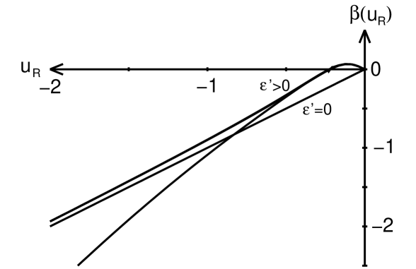
FIG. 3.: Approximations to the $\beta$ function of a directed polymer with periodic boundary conditions for a small $\epsilon^{\prime}$. The straight line is the limiting $\beta$ function $\beta(u_{R})=u_{R}$ for $\epsilon^{\prime}=0$. The other three are calculated with the same $\epsilon^{\prime}=0.005$ but truncated at different orders. Two of them already coincide.

4 Comparison between the perturbative and the transfer matrix approach

For harmonic boundary conditions, the zero of the $\beta$ function calculated by the regularized perturbative approaches is exactly equal to the finite size coefficient calculated in the transfer matrix picture.

Since the von-Neumann and Dirichlet boundary conditions in the transfer matrix approach and in the perturbation series are not absolutely equivalent (in the transfer matrix approach the boundary has a spherical shape), those results are not quantitatively comparable. Nevertheless qualitatively also those results are the same as far as the limit $\epsilon^{\prime}\to 0$ is concerned:

In the case of hard wall (Dirichlet) boundary conditions, the perturbation series predicts a $\beta$ function with a zero at a finite negative value. This is also the result of the transfer matrix calculation due to the finite value of the ground state energy of the free system.

With periodic (von-Neumann) boundary conditions, the perturbation theory and the transfer matrix approach both predict that ${\cal C}^{*}$ approaches zero as $\epsilon^{\prime}\to 0$ and they both result in the square root dependence (10) of $\epsilon^{\prime}$.

We can therefore conclude that the chosen method of regularization of the perturbation series reproduces the exact results of the transfer matrix approach and therefore is a valid regularization scheme.

III Arbitrary number of directed polymers

Now we will develop a diagrammatic expansion of the theory of an arbitrary number of directed polymers $N$ interacting by short range interactions. We will see that the structure shows strong analogies to the case of only two directed polymers, which suggests that the perturbation series can be regularized in the same way as the perturbation series for $N=2$.

A Diagrammatic expansion

1 Perturbation series of the partition function

In order to keep the calculations as simple as possible, we choose periodic boundary conditions as the infrared regularization. That means that we identify the points $r$ and $r+kL_{\perp}$ for every $k\in{\bf Z}^{d}$. Writing down the corresponding propagators, it is clear that the problem of $N$ directed polymers with periodic boundary conditions is equivalent to the problem of $N$ free directed polymers with periodic interactions.

So the perturbation series for the partition function remains the same as (26) with the definitions

$$\Phi(t)=\left(\sum_{i<j}^{N}\sum_{k_{ij}\in{\bf Z}^{d}}\delta(r_{i}(t)-r_{j}(t)-k_{ij}L_{\perp})\right)$$ (68)

and the free expectation values

$$\langle\cdot\rangle_{0}\equiv L_{\perp}^{-Nd}\!\!\!\!\!\int\limits_{[0,L_{\perp}]^{d}}\!\!\!\!\!{\rm d}^{d}r_{1}^{\prime}\ldots\!\!\!\!\!\int\limits_{[0,L_{\perp}]^{d}}\!\!\!\!\!{\rm d}^{d}r_{N}^{\prime}\int\limits_{{\bf R}^{d}}\!\!{\rm d}^{d}r_{1}^{\prime\prime}\ldots\!\!\int\limits_{{\bf R}^{d}}\!\!{\rm d}^{d}r_{N}^{\prime\prime}\!\!\!\!\int\limits_{(r_{1}^{\prime}\ldots,r_{N}^{\prime},0)}^{(r_{1}^{\prime\prime},\ldots,r_{N}^{\prime\prime},L_{||})}\!\!\!\!\!\!{\cal D}r_{1}\ldots{\cal D}r_{N}\cdot e^{-\frac{1}{2}\int_{0}^{L_{||}}\sum\limits_{i=1}^{N}\dot{r}_{i}^{2}(t){\rm d}t}$$ (69)

As in the above discussion, we first have to calculate the multi-point functions in the perturbation series of the partition function and combine them afterwards to the connected multi-point functions which are the integrands of the perturbation series of the free energy.

Since the argument of a multi-point function is the sum over different $\delta$ interactions, all sums can be extracted from the expectation value. In the $n$-th order the sums over $i<j$ correspond to the different ways, the $n$ interactions can be arranged among the $N$ directed polymers. Obviously a lot of arrangements are equivalent since for example interchanging the polymers that interact should not influence the expectation value of the sequence of interactions. So every possible arrangement of interactions will be accompanied by a combinatorial prefactor, which counts the number of equivalent arrangements. The sum over all $i<j$ can then be written as a sum over all possible arrangements with each arrangement multiplied by a convenient combinatorial prefactor.

Since there are obviously $N(N-1)\over 2$ possibilities to place the first interaction, all these prefactors will be multiples of $N(N-1)\over 2$. This is the reason, why we divide the free energy by this factor in order to get the renormalized coupling constant.

To improve the bookkeeping, we will represent every arrangement of interactions graphically by drawing parallel lines representing the directed polymers and a connection between two of them for every $\delta$ function between two polymers. The first connection belongs to the “time” $t_{1}$, the last one to the time $t_{n}$. To write down some simplified expressions later on, we also introduce a dotted line, which can represent a “time” in the diagram, where no interaction is present, and which is used to keep the relation between the time variables and the interactions, if an interaction is dropped due to a simplification rule.

Between two “interaction times” we have to insert the free propagator for $N$ directed polymers which of course factorizes in a product of free 1-polymer-propagators

$$G_{\Delta t}(r^{\prime},r^{\prime\prime}) = \int_{(r^{\prime},0)}^{(r^{\prime\prime},\Delta t)}{\cal D}re^{-\frac{1}{2}\int_{0}^{\Delta t}\dot{r}^{2}(t){\rm d}t}$$

$$= {1\over(2\pi\Delta t)^{\frac{d}{2}}}e^{-{(r^{\prime}-r^{\prime\prime})^{2}\over 2\Delta t}}$$

Since this is a Gaussian, all integrations over the $r_{i}$ can be performed. Moreover it is clear from the translational invariance of the propagator that only a dependence on “time” differences will arise. Therefore we change our integration variables. Instead of integrating over all ordered “times” $0<t_{1}<\ldots<t_{n}<L_{||}$, we integrate over all existing “time” differences $t_{i}-t_{i-1}$. In the limit of infinitely long directed polymers ($L_{||}\to\infty$) the domain of integration is from zero to infinity for each of these variables, whereas the integration over $t_{1}$ just gives a factor of $L_{||}$ which is canceled because we want to calculate the free energy per length and per pair of directed polymers. The new integration variables will be made dimension-less by a factor of $L$ and we call them $s_{1},\ldots,s_{n-1}$.

To calculate the integrands, some simplification techniques can be used and especially two general simplification rules, which we will call lemma A and B can be derived. The integrands of the first three orders of the perturbation series for the partition function can be explicitly calculated by using these techniques. The detailed simplification rules and the calculation for the first three orders can be found in appendix G and lead to

$${2\over N(N-1)}\langle\Phi(t)\rangle_{0}=L_{\perp}^{-d},$$ (70)

$${2\over N(N-1)}\langle\Phi(0)\Phi(Ls_{1})\rangle_{0}=L_{\perp}^{-d}R^{p}(s_{1})+{(N-1)(N-2)\over 2}L_{\perp}^{-2d},$$ (71)

and

$${2\over N(N-1)}\langle\Phi(0)\Phi(Ls_{1})\Phi(L(s_{1}+s_{2}))\rangle_{0} = L_{\perp}^{-d}R^{p}(s_{1})R^{p}(s_{2})+{(N+1)(N-2)\over 2}L_{\perp}^{-2d}R^{p}(s_{1})$$ (75)

$$+{(N+1)(N-2)\over 2}L_{\perp}^{-2d}R^{p}(s_{2})$$

$$+{(N+5)(N-2)\over 2}L_{\perp}^{-2d}R^{p}(s_{1}+s_{2})$$

$$+{(N-2)(N-3)(N^{2}+3N+4)\over 4}L_{\perp}^{-3d}$$

with the two-polymer return probability

$$R^{p}(s)=\left(\frac{1}{\sqrt{L}}\sum_{k\in{\bf Z}}e^{-4\pi k^{2}s}\right)^{d}.$$ (76)

We want to stress at this point that up to the third order the only quantity arising is the two-polymer return probability $R^{p}(s)$ and the only effect of more than two directed polymers are the combinatorial prefactors. Unfortunately we cannot just stop our discussion here, because in the forth order, generically new diagrams arise. Since the number of diagrams heavily increases, it is convenient to use some computer algebra in order to generate all diagrams. In the sixth order for example there are 29388 possible arrangements of the interactions, which can be reduced to 5300 by automatically applying lemma A.

The new diagrams in the forth order are the following ones

They can of course also be integrated out, which gives $L_{\perp}^{-3d}R^{p}(s_{1}+2s_{2}+s_{3})$ for the first one. The other two contain two sums over ${\bf Z}^{d}$ that cannot be decoupled. The second one for example reads

$$\left\{{1\over 4\pi L^{2}}\left[{\rm det}\left(\begin{array}[]{cc}s_{1}+s_{2}+s_{3}&\frac{1}{2}s_{2}\\ \frac{1}{2}s_{2}&s_{2}\end{array}\right)\right]^{-\frac{1}{2}}\sum_{k,k^{\prime}\in{\bf Z}}e^{-{(k\,k^{\prime})\left(\begin{array}[]{cc}t_{1}+t_{2}+t_{3}&\frac{1}{2}t_{2}\\ \frac{1}{2}t_{2}&t_{2}\end{array}\right){k\choose{k^{\prime}}}\over{\textstyle 4\rm det}\left(\begin{array}[]{cc}\scriptstyle s_{1}+s_{2}+s_{3}&\scriptstyle\frac{1}{2}s_{2}\\ \scriptstyle\frac{1}{2}s_{2}&\scriptstyle s_{2}\end{array}\right)}}\right\}^{d}$$ (77)

Here it is already written in a form that makes it obvious that it is connected to a two-dimensional theta function and that it can be simplified by applying the corresponding transformation formula [27] to

$\displaystyle\left\{{1\over L^{2}}\sum_{k,k^{\prime}\in{\bf Z}}e^{-4\pi^{2}{{\textstyle(k\,k^{\prime})}\left(\begin{array}[]{cc}s_{1}+s_{2}+s_{3}&\frac{1}{2}s_{2}\\ \frac{1}{2}s_{2}&s_{2}\end{array}\right)\left(\begin{array}[]{c}k\\ k^{\prime}\end{array}\right)}}\right\}^{d}$Calculating the diagrams to higher orders shows us that there is a simple recipe, that allows to perform all spatial integrations formally, if the form of the diagram is given. The rules are as follows:

1. Mark all loops in the diagram that are necessary to pass each interaction at least with one loop. Assign an orientation to every loop.

2. If there are $m$ loops necessary, use an $m\times m$ matrix T and identify each row and column with one of the loops

3. pass for all “time” intervals $i$ over all lines of the diagram and

   • add $\frac{1}{2}s_{i}$ to every diagonal element of a loop, that passes the line

   • add $\pm\frac{1}{2}s_{i}$ to both of the off diagonal elements of two loops, that pass together through the line. If they pass in the same orientation the plus sign has to be used, otherwise the minus sign.

4. The value of the diagram is then

   $$\left[L^{-{{\rm order}\over 2}}\sum_{k\in{\bf Z}^{m}}e^{-4\pi^{2}k^{T}Tk}\right]^{d}.$$ (78)

This prescription also implies the validity of the lemmas A and B used above.

Since there are several possibilities to choose the loops in a diagram, the correspondence from a diagram to a T-matrix is not unique. For example in the forth order diagram, the loops could be chosen as:

which leads to the T-matrices

$\displaystyle\left(\begin{array}[]{cc}t_{1}+t_{2}&\frac{1}{2}t_{2}\\ \frac{1}{2}t_{2}&t_{2}+t_{3}\end{array}\right)\quad\hbox{and}\quad\left(\begin{array}[]{cc}t_{1}+t_{2}+t_{3}&\frac{1}{2}t_{2}+t_{3}\\ \frac{1}{2}t_{2}+t_{3}&t_{2}+t_{3}\end{array}\right).$Although the T-matrices are not identical, the sums, which determine the value of the T-matrix are the same, because the second of those matrices is reproduced, if in the sum with the first matrix, the summation variable $k_{2}$ is shifted by $k_{1}$. During all those equivalence transformations, the determinant of the T-matrix does not change, so that two T-matrices from different diagrams can only be equivalent, if their determinants are identical. Unfortunately there exist also T-matrices which are not equivalent but have the same determinant.

Since the whole procedure described above is purely mechanical, it can be implemented by computer algebra. The only thing left to do is manually checking the equivalence of T-matrices which have the same determinant. This reduces the number of different diagrams in the fifth order from 348 to 88.

2 Perturbation series of the free energy

Since we now know how to compute the multi-point functions, we can calculate the free energy using the formula from appendix B. Analogous to the connected two point functions we used for the 2 polymer problem, we have to express everything in terms of correlation functions, that decay properly for increasing time differences. In analogy to the definition of $g_{1}$, which in our terminology reads $g_{1}(s)=L_{\perp}^{d}R^{p}(s)-1$, we will use functions of T-matrices, where all sub-matrices of lower dimensions are subtracted with alternating signs, as for example

$$g_{2}(a,b,c) \equiv \left\{\sum_{k\in{\bf Z}^{2}}e^{-4\pi^{2}k^{T}\left(\begin{array}[]{cc}a&b\\ b&c\end{array}\right)k}\right\}^{d}$$

$$-\left\{\sum_{k\in{\bf Z}}e^{-4\pi^{2}ak^{2}}\right\}^{d}-\left\{\sum_{k\in{\bf Z}}e^{-4\pi^{2}ck^{2}}\right\}^{d}+1,$$

and analogously for a higher number of loops.

Of course the subtracted terms depend on the T-matrix itself and are different, if one chooses different T-matrices which represent the same diagram (which give the same value for the first term of the above sum). If one chooses the wrong representation, one will discover that there are terms, the time integrals of which will not converge. But it is always possible to choose a representation, that leads to terms which are each integrable (of course the sum of all terms is integrable in every case, it is just possible that one chooses an inconvenient partition of the integrand.)

Once the coefficients of the free energy are represented as a sum over time integrals, further simplifications can be performed, by multiplying the integration variables by constant factors and applying all kinds of relations as the ones discussed in appendix C.

We will continue to represent every of those integrals by one of the diagrams, which is responsible for the main term of the integrand. Since the integrands themselves depend on the way, the loops are chosen, we must specify our choice. Those parts of diagrams, which can be expressed only by $g_{1}$ (i.e. which are pure 2-polymer-diagrams) will be represented by the same diagrams as they have been used in the 2 polymer case.

The resulting diagrammatic expansion for the free energy is shown in Fig. 4 up to the fifth order.

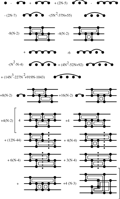
FIG. 4.: Diagrammatic series expansion of the free energy per length up to the fifth order for an arbitrary number $N$ of interacting polymers.

It should be stressed that the number of diagrams involved in this final expansion is very small compared to the number of diagrams in the original perturbation series of the partition function. Since the applicability of most of the simplifying formulas as those from appendix C relies on very specific relations between the coefficients of the diagrams involved, it is very unlikely that this structure evolves just by chance. This is a strong hint that there exists a similar equation as (41) for an arbitrary number of directed polymers, that produces this relatively simple structure of the perturbation series. Unfortunately no such formula could be found up to now.

B Comparison with the $N=2$ case

We can now compare the perturbation series to the perturbation series of two directed polymers.

First there are a lot of diagrams which appear already in the series of two directed polymers, that now have prefactors with a polynomial $N$ dependence. We will call them “linear” diagrams, because they have no nested loops. The value of one arc itself is of course the same as for two directed polymers. Especially only the arc, that spans two intervals has a pole at $\epsilon^{\prime}\to 0$. This pole is of the first order.

Since we have explicit expressions for all of the diagrams, it is also possible to extract at least the order of the pole of each of the nested diagrams as $\epsilon^{\prime}\to 0$. This can be done by extracting the UV dependence of the integrands and partial integration. It comes out that all nested diagrams are less divergent than the product of two-interval arcs in the same order of the perturbation theory.

Therefore, as in the case of two directed polymers, the powers of the two-interval arc are the most divergent diagrams and the order of the pole grows by one only in every second order of the perturbation series.

Although we gave here the diagrammatic expansion of the series $u_{R}(u_{0})$, the same statements are true for the inverted series $u_{0}(u_{R})$, since it consist of exactly the same diagrams with other prefactors.

Analogous to the case of two directed polymers, we write the partial sum over all those most divergent diagrams as

$${u_{0}(u_{R})\over\epsilon^{\prime}}={1\over u_{R}}f_{reg}\left(u_{R}\over\sqrt{\epsilon^{\prime}}\right)+\mbox{less divergent terms}$$ (80)

where $f_{reg}$ is an even function, with Taylor coefficients, that stay regular as $\epsilon^{\prime}\to 0$. If we now assume that the fact that the series for $f_{reg}(x)$ can be analytically continued to $x\to\infty$ and that $\lim_{x\to\infty}f_{reg}(x)$ exists is not a particularity of 2 directed polymers, we get a leading behavior of

$${u_{0}(u_{R})\over\epsilon^{\prime}}\approx{a\over u_{R}}\hbox{ with }a=\lim\limits_{x\to\infty}f_{reg}(x)$$ (81)

Differentiation then leads to the limiting $\beta$ function

$$\beta(u_{R})=u_{R}+\hbox{higher order terms.}$$ (82)

The slope of $1$ of this $\beta$ function shows that $u_{R}=0$ is not just the Gaussian fixed point, which would have a slope of $\epsilon=-1$. Thus we expect that for $\epsilon^{\prime}\to 0$ the non-Gaussian fixed point goes to zero for each $N$. Since the $\beta$ function is a regular function of $u_{R}/\sqrt{\epsilon^{\prime}}$ also the behavior proportional to $\sqrt{\epsilon^{\prime}}$ is independent of $N$.

C Consequences for the limit $N\to 0$

The independence of the behavior of the fixed point near $d=4$ renders the limit $N\to 0$, which describes the directed polymer in a random medium, trivial. Thus we easily conclude that the finite size amplitude of the free energy per unit “time” also vanishes as given in equation (10) for the directed polymer in a random medium.

This shows that the singularities in the perturbation series, which arise at $d=4$ are not only a formal problem of the approach, but they lead to a non-analytic behavior of a physical quantity.

Although we are surely not able to access the strong coupling fixed point of the KPZ equation with these perturbative methods, the shown vanishing of the weak coupling fixed point, which is under the Hopf–Cole transformation equivalent to the studied interaction fixed point in the directed polymer picture, is a strong hint that $4$ is really the upper critical dimension for the KPZ problem.

Although the duality relations between dimensions $d$ and $4-d$ in section II C 2 only have been observed in the case $N=2$, one could speculate that such a relationship still exists for arbitrary $N$ and the KPZ problem. This is especially interesting since Frey and Täuber find in [29, 10] that their coupling constant approaches zero in the limit $d\to 0$. Surely it is not absolutely clear how the two coupling constants are related and this point deserves further investigations.

IV Conclusion and outlook

We have studied the problem of directed polymers with short range interactions. The main interest was the behavior of the directed polymer system in the limit $d\to 4$, where the normal renormalization treatment, which expands around $d=2$ breaks down. Since for two directed polymers exact transfer matrix results are available, we developed a regularization procedure for the perturbation series in the limit $d\to 4$ in the special case of two directed polymers. We could prove that there is an agreement between the transfer matrix results and the predictions of the regularized perturbation series for two directed polymers. Moreover an exact implicit equation which generates the whole perturbation series and its connections to the diagrammatic expansion has been studied.

For an arbitrary number of directed polymers, a diagrammatic expansion of the free energy up to the fifth order has been established. Although it stems from a large number of terms this expansion is relatively simple. This suggests that it can also be generated by a simple equation, which has, however, eluded us so far. Since the pole structure of the perturbation series is very similar to the pole structure in the case $N=2$, the leading behavior of the $\beta$ function in the limit $d\to 4$ has been derived. It shows that the interaction fixed point approaches zero as $d\to 4$ proportional to $\sqrt{\epsilon^{\prime}}$ independent of $N$. Therefore the weak coupling fixed point of the KPZ equation (which is mapped to the problem of a directed polymer in a random medium) is also expected to approach 0 proportional to $\sqrt{\epsilon^{\prime}}$ in the limit $d\to 4$.

For $d>4$ the transfer matrix calculations show for two directed polymers, that the finite size amplitude of the free energy per unit “time” at the unbinding transition develops anomalous scaling behavior analogous to that of the free energy in the bound state of the infinite system [19, 20]. The finite size amplitude therefore depends explicitly on the short-distance cutoff. Thus it is no longer possible to define a universal quantity from the free energy. If this behavior persists for arbitrary $N$, the critical behavior of the KPZ equation at the roughening transition above $d=4$ is less universal than below 4 dimensions.

We conclude by noting that the unbinding transition of semi-flexible polymers (i.e. directed lines which are governed by the curvature instead of a line tension) with a short-ranged attraction of parallel polymer segments in one transversal dimension formally can be mapped on the problem of two strings in four transversal dimensions. Therefore the method studied here can also be applied to examine this unbinding transition [30].

A Solutions of the radial Schroedinger equation with constant potential

We have to calculate the asymptotic behavior of the ground state energy, which belongs to the rescaled version

$\displaystyle\left\{-{\partial^{2}\over\partial y^{2}}+{(d-3)(d-1)\over 4}{1\over y^{2}}+\bar{V}(y)\right\}\phi(y)=E_{0}\phi(y)$of the radial equation (14). The rescaled potential is

$$\bar{V}(r)=\left\{\begin{array}[]{rl}-V_{0}&0\leq r<1\\ 0&1\leq r\end{array}\right.,$$ (A1)

where $\phi(r)=\Phi(ra)$, $E_{0}=a^{2}\tilde{E}_{0}$, $\bar{V}(r)=a^{2}V(ra)$ and $V_{0}=a^{2}\tilde{V}_{0}$.

Obviously the wave function must consist of general solutions of the Schroedinger equation with constant potential.

$$\left(-{\partial^{2}\over\partial y^{2}}+{(d-3)(d-1)\over 4}{1\over y^{2}}-E\right)\phi(y)=0$$ (A2)

The general solution of this differential equation is [24]

$\displaystyle\phi(y)=\left\{\begin{array}[]{cc}A\sqrt{y}J_{|\epsilon|}(y\sqrt{E})+B\sqrt{y}N_{|\epsilon|}(y\sqrt{E})&E>0\\ Ay^{d-1\over 2}+By^{3-d\over 2}&E=0\\ A\sqrt{y}I_{|\epsilon|}(y\sqrt{-E})+B\sqrt{y}K_{|\epsilon|}(y\sqrt{-E})&E<0\end{array}\right..$

Because the wave function should be regular at the origin at least for $d>2$ only the first solution is possible for the interaction region. This means that for $y\leq 1$

$$\phi(y)=\left\{\begin{array}[]{cc}A\sqrt{y}J_{|\epsilon|}(y\sqrt{E_{0}+V_{0}})&E_{0}+V_{0}>0\\ A\sqrt{y}y^{|\epsilon|}&E_{0}+V_{0}=0\\ A\sqrt{y}I_{|\epsilon|}(y\sqrt{-E_{0}-V_{0}})&E_{0}+V_{0}<0\end{array}\right..$$ (A3)

In the outer region the boundary conditions at $y=L/a$ lead to the wave functions

$\displaystyle\phi(y)=B[\sqrt{y}J_{|\epsilon|}(y\sqrt{E_{0}})-g_{|\epsilon|}(\sqrt{E_{0}}\frac{L}{a})\sqrt{y}N_{|\epsilon|}(y\sqrt{E_{0}})]$for $E_{0}>0$,

$\displaystyle\phi(y)=\left\{\begin{array}[]{ll}B[y^{d-1\over 2}-\left(L\over a\right)^{d-2}y^{3-d\over 2}]&\mbox{ Dirichlet}\\ By^{d-1\over 2}&\mbox{ von-Neumann}\end{array}\right.$for $E_{0}=0$, and

$\displaystyle\phi(y)\!=\!B[\sqrt{y}I_{|\epsilon|}(y\sqrt{-E_{0}})-f_{|\epsilon|}(\sqrt{-E_{0}})\sqrt{y}K_{|\epsilon|}(y\sqrt{-E_{0}})]$for $E_{0}<0$ respectively with

$$f_{|\epsilon|}(x)=\left\{\begin{array}[]{ll}I_{|\epsilon|}(x)\over K_{|\epsilon|}(x)&\hbox{Dirichlet}\\ -{I_{|\epsilon|+1}(x)\over K_{|\epsilon|+1}(x)}&\hbox{von-Neumann}\end{array}\right.$$ (A4)

and

$$g_{|\epsilon|}(x)=\left\{\begin{array}[]{ll}J_{|\epsilon|}(x)\over N_{|\epsilon|}(x)&\hbox{Dirichlet}\\ {J_{|\epsilon|+1}(x)\over N_{|\epsilon|+1}(x)}&\hbox{von-Neumann}\end{array}\right..$$ (A5)

The total solution consists of these two solutions if they obey the condition of continuous differentiability, which is most conveniently written as

$\displaystyle\phi(1-)=\phi(1+)$and

$\displaystyle\phi^{\prime}(1-)-(|\epsilon|+\frac{1}{2})\phi(1-)=\phi^{\prime}(1+)-(|\epsilon|+\frac{1}{2})\phi(1+).$Since this are two conditions for the two free coefficients $A$ and $B$, we only get a solution for energies, where the determinant of the linear system of equation vanishes. This gives us the equation connecting $E_{0}$ with $V_{0}$ and $L_{\perp}\over a$.

This equation will always have the form

$$r(\sqrt{\pm E_{0}}\frac{L_{\perp}}{a})=s(\sqrt{\pm E_{0}})$$ (A6)

with some functions $r$ and $s$. Since the ground state energy is expected to vanish for $L_{\perp}\to\infty$ at least proportional to $(a/L_{\perp})^{2}$, we have to distinguish two cases which are determined by the value of $s_{0}\equiv\lim_{x\to 0}s(x)$. If $s_{0}$ is a finite value, $E_{0}$ will asymptotically decay as $\pm c^{2}(a/L_{\perp})^{2}$, where $c$ is the smallest positive solution of $r(x)=s_{0}$. So $c^{2}$ is exactly the coefficient, we are interested in. If $s_{0}=0$, the constant $c$ is a root of $r(x)$. Since $r(0)=0$, $c$ can be zero, but only if the signs of $r$ and $s$ for small positive arguments are equal. If not, $c$ is the smallest positive root of $r$. If $c$ is zero, one can expand $r$ for small arguments and furthermore extract the leading behavior in $a/L_{\perp}$ of $E_{0}$, which then decays faster than quadratic.

Since we are especially interested in the asymptotic behavior of the ground state energy at the phase transition point $V_{*}$, we have to identify it. It is defined by the condition that the ground state energy in an infinite system approaches zero from below. Since we know the solutions of the Schroedinger equation in the interaction region and outside (for $L_{\perp}\to\infty$ only the regular solution proportional to $K_{|\epsilon|}$ is possible), we can exploit the matching conditions for $E_{0}+V_{*}>0$ and $E_{0}<0$ and take the limit $E_{0}\to 0$, which gives

$${J_{|\epsilon|+1}(\sqrt{V_{*}})\sqrt{V_{*}}\over J_{|\epsilon|}(\sqrt{V_{*}})}=2|\epsilon|.$$ (A7)

We now can systematically apply the above scheme to all possible combinations $V_{0}=0$, $0<V_{0}<V_{*}$ and $V_{0}=V_{*}$, $E_{0}<-V_{0}$, $E_{0}=V_{0}$, $-V_{0}<E_{0}<0$, $E_{0}=0$ and $E_{0}>0$ and both boundary conditions and extract all possible values of the coefficient $c$. The smallest one is the ground state energy.

The only point, which has to be handled with care during this calculation is the series expansion of the different Bessel functions involved. Since especially for $V_{0}=V_{*}$ the leading terms of the expansions cancel, the sub-leading terms have to be used. But the sub-leading terms are of totally different origin if $|\epsilon|>1$ or $|\epsilon|<1$. This produces the difference of the ground state energies in $d>4$ and $d<4$ as we expect them.

B Expansion of the free energy

Since we need it during the calculations, we give here the expansion of the free energy per length written by $n$ point functions up to the forth order. It is:

$$\lim\limits_{L_{||}\to\infty}\!\!{F(g)-F(0)\over L_{||}} = g\langle\Phi(0)\rangle_{0}-g^{2}\int_{0}^{\infty}\langle\Phi(0)\Phi(t)\rangle_{0}-\langle\Phi(0)\rangle_{0}^{2}{\rm d}t+$$

$$+ g^{3}\int\int\limits_{\hbox to0.0pt{\hss$\scriptstyle 0\leq t_{1}\leq t_{2}$ }}{\rm d}t_{1}{\rm d}t_{2}\Bigg{[}\langle\Phi(0)\Phi(t_{1})\Phi(t_{2})\rangle_{0}-\langle\Phi(0)\rangle_{0}\langle\Phi(t_{1})\Phi(t_{2})\rangle_{0}$$

$$\qquad-\langle\Phi(t_{1})\rangle_{0}\langle\Phi(0)\Phi(t_{2})\rangle 0-\langle\Phi(t_{2})\rangle_{0}\langle\Phi(0)\Phi(t_{1})\rangle_{0}+2\langle\Phi(0)\rangle_{0}^{3}\Bigg{]}$$

$$- g^{4}\!\!\int\int\int\limits_{\hbox to0.0pt{\hss$\scriptstyle 0\leq t_{1}\leq t_{2}\leq t_{3}$}}{\rm d}t_{1}{\rm d}t_{2}{\rm d}t_{3}\Bigg{[}\langle\Phi(0)\Phi(t_{1})\Phi(t_{2})\Phi(t_{3})\rangle_{0}-\!\langle\Phi(0)\Phi(t_{1})\rangle_{0}\langle\Phi(t_{2})\Phi(t_{3})\rangle_{0}$$

$$\qquad\qquad-\langle\Phi(0)\Phi(t_{2})\rangle_{0}\langle\Phi(t_{1})\Phi(t_{3})\rangle_{0}-\langle\Phi(0)\Phi(t_{3})\rangle_{0}\langle\Phi(t_{1})\Phi(t_{2})\rangle_{0}$$

$$\qquad\qquad-\langle\Phi(0)\rangle_{0}\langle\Phi(t_{1})\Phi(t_{2})\Phi(t_{3})\rangle_{0}-\langle\Phi(0)\rangle_{0}\langle\Phi(0)\Phi(t_{2})\Phi(t_{3})\rangle_{0}$$

$$\qquad\qquad-\langle\Phi(0)\rangle_{0}\langle\Phi(0)\Phi(t_{1})\Phi(t_{3})\rangle_{0}-\langle\Phi(0)\rangle_{0}\langle\Phi(0)\Phi(t_{1})\Phi(t_{2})\rangle_{0}$$

$$\qquad\qquad+2\langle\Phi(0)\Phi(t_{1})\rangle_{0}\langle\Phi(0)\rangle_{0}^{2}+2\langle\Phi(0)\Phi(t_{2})\rangle_{0}\langle\Phi(0)\rangle_{0}^{2}$$

$$\qquad\qquad+2\langle\Phi(0)\Phi(t_{3})\rangle_{0}\langle\Phi(0)\rangle_{0}^{2}+2\langle\Phi(t_{1})\Phi(t_{2})\rangle_{0}\langle\Phi(0)\rangle_{0}^{2}$$

$$\qquad\qquad+2\langle\Phi(t_{1})\Phi(t_{3})\rangle_{0}\langle\Phi(0)\rangle_{0}^{2}+2\langle\Phi(t_{2})\Phi(t_{3})\rangle_{0}\langle\Phi(0)\rangle_{0}^{2}-6\langle\Phi(0)\rangle_{0}^{4}\Bigg{]}$$

$$+ O(g^{5}).$$

In the case of only two directed polymers, this whole series can be reexpressed only by connected two point functions and then represented diagrammatically as explained in section II B. It reads then:

C Proving relations among diagrams

Every diagram is related to a multiple “time” integral over a product of connected two point functions, the arguments of which are sums of the different integration variables. If we assume that the two point function can be Laplace transformed, general rules among the diagrams can be proved. We will show with one example how this proceeds. We introduce the Laplace transform $\hat{g}_{1}$ of $g_{1}$. Then:

$\displaystyle\int_{0}^{\infty}ds_{1}\int_{0}^{\infty}ds_{2}\int_{0}^{\infty}ds_{3}g_{1}(s_{1}+s_{2}+s_{3})g_{1}(s_{2})+\int_{0}^{\infty}ds_{1}\int_{0}^{\infty}ds_{2}\int_{0}^{\infty}ds_{3}g_{1}(s_{1}+s_{2})g_{1}(s_{2}+s_{3})=$

$${1\over(2\pi i)^{2}}\int_{c}dz_{1}\int_{c}dz_{2}\hat{g}_{1}(z_{1})\hat{g}_{1}(z_{2})\int_{0}^{\infty}ds_{1}\!\int_{0}^{\infty}ds_{2}\!\int_{0}^{\infty}ds_{3}\Big{[}\frac{1}{2}e^{z_{1}(s_{1}+s_{2}+s_{3})+z_{2}s_{2}} + \frac{1}{2}e^{z_{1}s_{2}+z_{2}(s_{1}+s_{2}+s_{3})}$$

$$+ e^{z_{1}(s_{1}+s_{2})+z_{2}(s_{2}+s_{3})}\Big{]}$$

From its definition $c$ is a path parallel to the imaginary axis with positive real part. In order to be able to interchange the integrations, we have used that the inner integrals exist, which is of course only true, if the real parts of the $z_{i}$ are negative. But since the connected correlation functions decay exponentially for large arguments, the Laplace transform $\hat{g}_{1}$ is still analytic in some region to the left of the imaginary axis and the integration contour can be shifted there without changing the value of the integral.

After doing so, we can evaluate the integrals over the exponentials and get

$$\ldots\!\! = {1\over(2\pi i)^{2}}\int_{c}dz_{1}\int_{c}dz_{2}\hat{g}_{1}(z_{1})\hat{g}_{1}(z2)\left[-{1\over 2z_{1}^{2}(z_{1}+z_{2})}-{1\over 2z_{2}^{2}(z_{1}+z_{2})}-{1\over z_{1}z_{2}(z_{1}+z_{2})}\right]$$

$$= {1\over(2\pi i)^{2}}\int_{c}dz_{1}\int_{c}dz_{2}\hat{g}_{1}(z_{1})\hat{g}_{1}(z_{2})\left(-{z_{1}+z_{2}\over 2z_{1}^{2}z_{2}^{2}}\right)={1\over(2\pi i)^{2}}\int_{c}dz_{1}\int_{c}dz_{2}\hat{g}_{1}(z_{1})\hat{g}_{1}(z_{2})\left(-{1\over z_{1}^{2}z_{2}}\right)$$

$$= {1\over(2\pi i)^{2}}\int_{c}dz_{1}\int_{c}dz_{2}\hat{g}_{1}(z_{1})\hat{g}_{1}(z_{2})\int_{0}^{\infty}ds_{1}\int_{0}^{\infty}ds_{2}\int_{0}^{\infty}ds_{3}e^{z_{1}(s_{2}+s_{3})+z_{2}s_{1}}$$

$$= \int_{0}^{\infty}ds_{1}\int_{0}^{\infty}ds_{2}\int_{0}^{\infty}ds_{3}g_{1}(s_{1})g_{1}(s_{2}+s_{3}).$$

The diagrammatic expression for this equation is the one in section II B.

D Derivation of the exact implicit equation for the free energy

Using the abbreviations from section II C the $n$-th order term of the partition function series is expressed by

$${1\over{\cal N}}\int_{0}^{L_{||}}{\rm d}t_{n}\int_{0}^{t_{n}}{\rm d}t_{n-1}\ldots\int_{0}^{t_{2}}{\rm d}t_{1}$$

$$g(t_{1})f(t_{2}-t_{1})\ldots f(t_{n}-t_{n-1})h(L_{||}-t_{n})$$

Laplace transforming this with respect to $L_{||}$ yields $\hat{g}(z)\hat{f}(z)^{n-1}\hat{h}(z)$ for the Laplace transforms.

Obviously the Laplace transformed perturbation series is just a geometric series and can therefore be resummed. After back-transformation we end up with

$${Z\over Z_{0}}-1=-{g\over 2\pi i{\cal N}}\int_{c}{\hat{g}(z)\hat{h}(z)\over 1+g\hat{f}(z)}e^{L_{||}z}{\rm d}z,$$ (D1)

where $c$ is a path in the complex plane parallel to the imaginary axis. Since we can obviously close this path by a circle at $z\to-\infty$, the integral is given as the sum of the residues of the integrand in the half plane of negative real parts. From the form of the integrand it is clear that all residues will be some prefactor times an exponential with the position of the pole times $L_{||}$ as its argument. In the limit of $L_{||}\to\infty$ only the pole with the smallest decay rate (i.e. the one with the smallest absolute value of its real part) survives.

By construction, it is clear that ${\cal N}$ has a leading dependence on $L_{||}$ of $e^{-L_{||}\ln Z_{0}}$, whereas the poles of $\hat{g}$ and $\hat{h}$ are exactly the negative eigenvalues of the Schroedinger operator corresponding to the free directed polymer problem (described by ${\cal H}_{0}$). The smallest eigenvalue is the leading term of $\ln Z_{0}$ itself, the contribution of which to the integral must cancel against the $1$ on the left hand side.

From that we conclude that the leading term of $Z$ for large $L_{||}$ is some prefactor times $\exp(z_{0}L_{||})$, where $z_{0}$ is the solution of the equation

$$1+g\hat{f}(z)=0$$ (D2)

with the largest (absolutely smallest) real part. This decay rate is therefore the leading contribution to the free energy per length in the limit $L_{||}\to\infty$.

E Hard wall return probability

To calculate the return probability of a $1+d$-dimensional directed polymer in a round box, we can use the “quantum mechanical” expression of the propagator by the eigenfunctions of the “particle in a box” problem. The eigenfunctions of the particle in a box are Bessel functions of the first kind and for $d>2$ we get with the correct normalization conditions

$$G_{t}({\bf r},{\bf r}^{\prime})={2\over L_{\perp}^{2}}\sum_{l=0}^{\infty}\sum_{J_{{d-2\over 2}+l}(\alpha L_{\perp})=0}\!\!\!\!\!\!\!\!\!\!e^{-{\alpha^{2}\over 2}t}\sum_{m}\omega^{*}_{l,m}(\Omega_{\bf r})\omega_{l,m}(\Omega_{\bf r^{\prime}}){r^{2-d\over 2}J_{{d-2\over 2}+l}(\alpha r){r^{\prime}}^{2-d\over 2}J_{{d-2\over 2}+l}(\alpha r^{\prime})\over\left[J_{{d-2\over 2}+l+1}(\alpha L_{\perp})\right]^{2}},$$ (E1)

which for $d=3$ is the heat equation kernel in [28].

In the limit $r\to 0$, which we need for the return probability, only the $l=0$ terms stay finite. The sum over the for $l=0$ radially symmetric eigenfunctions of the angular momentum operator is just one over the surface of the $d$-dimensional unit sphere. Thus the return probability is

$${\Gamma(\frac{d}{2})\over\pi^{d/2}L_{\perp}^{2}}\sum_{J_{d-2\over 2}(\alpha L_{\perp})=0}{e^{-{\alpha^{2}\over 2}t}\left(\alpha\over 2\right)^{d-2}\over\left[J_{\frac{d}{2}}(\alpha L_{\perp})\right]^{2}}.$$ (E2)

Its Laplace transform can formally be calculated term by term, but since we know that it is ultraviolet divergent for $d>2$ we introduce a lower cutoff $a$ of the integration, which give

$${\Gamma(\frac{d}{2})\over\pi^{d/2}(2L_{\perp})^{d-2}}e^{-az}\sum_{J_{d-2\over 2}(\alpha)=0}{\alpha^{d-2}\over\left[J_{\frac{d}{2}}(\alpha)\right]^{2}}{e^{-{a\over L_{\perp}^{2}}{\alpha^{2}\over 2}}\over zL_{\perp}^{2}+{\alpha^{2}\over 2}}.$$ (E3)

In the prefactor the limit $a\to 0$ is possible without any difficulties.

If we now specialize to the case $d=3$, where the roots of the Bessel function are just the integer multiples of $\pi$, we can insert the especially simple expressions for the Bessel functions and end up with

$$\pi\sum_{n=1}^{\infty}{e^{-a{\pi^{2}n^{2}\over 2}}\over 1+{2zL_{\perp}^{2}\over\pi^{2}n^{2}}} = \pi\sum_{n=1}^{\infty}e^{-a{\pi^{2}n^{2}\over 2}}\sum_{k=0}^{\infty}\left(-{2zL_{\perp}^{2}\over\pi^{2}n^{2}}\right)^{k}$$

$$= \pi\sum_{k=0}^{\infty}\left(-{2\over\pi^{2}}\right)^{k}(zL_{\perp}^{2})^{k}\sum_{n=1}^{\infty}{e^{-a{\pi^{2}n^{2}\over 2}}\over n^{2k}},$$

where we have absorbed a factor of $1/L_{\perp}^{2}$ into $a$ and omitted the geometrical prefactor. For $k\geq 1$ the limit $a\to 0$ is possible and we get

$$\pi\sum_{n=1}^{\infty}e^{-a{\pi^{2}n^{2}\over 2}}+\pi\sum_{k=1}^{\infty}\left(-{2\over\pi^{2}}\right)^{k}\zeta(2k)(zL_{\perp}^{2})^{k}$$

$$= \pi\sum_{n=1}^{\infty}e^{-a{\pi^{2}n^{2}\over 2}}-{\pi\over 2}\left[L_{\perp}\sqrt{-2z}\cot(L_{\perp}\sqrt{-2z})-1\right].$$

The last equation can be verified by representing the values of the $\zeta$ function by Bernoulli numbers which gives exactly the series expansion of the cotangent function. The $k=0$ sum obviously diverges for $a\to 0$. If we add $\frac{\pi}{2}$, it is half of the value of theta function at zero, which diverges like $a^{-\frac{1}{2}}$ with no sub-leading algebraic terms. So, if we ignore the divergence, the first sum contributes $-\frac{\pi}{2}$ to the return probability. Thus the regularized Laplace transform of the return probability is

$$-{1\over 8}\sqrt{-2z}\cot(L_{\perp}\sqrt{-2z}),$$ (E4)

if we add all the geometrical prefactors again. This leads to the equation for the free energy per length of the system with a short range interaction cited in the main text.

F Explicit regularization of the perturbation series

If we insert the Laurent expansions of the coefficients $a_{i}$ into the perturbation expansion of $u_{0}(u_{R})\over\epsilon\prime$, we get a regular part of this series to the leading orders in $u_{R}$ of

$\displaystyle a_{1,1}u_{R}^{2}+(a_{2,1}+2a_{1,-1}a_{1,2}+2a_{1,0}a_{1,1})u_{R}^{3}+O(u_{R}^{4})$As discussed in the main text, the singular parts has a quite simple structure. All terms of the same divergence order can be combined to geometric series with polynomial prefactors. The most singular terms (the first three divergence orders) are

$$\left(a_{1,-1}u_{R}\over\epsilon^{\prime}\right)^{n}\! \!\Big{\{}\! {1\over a_{1,-1}}+\left[n{a_{1,0}\over a_{1,-1}}+(n-1){a_{2,-1}\over(a_{1,-1})^{2}}\right]u_{R}+$$

$$+ \Big{[}(n+1)a_{1,1}+n{a_{2,0}\over a_{1,-1}}+n{a_{2,0}\over a_{1,-1}}+{n(n+1)\over 2}{(a_{1,0})^{2}\over a_{1,-1}}$$

$$\quad+(n^{2}-n){a_{1,0}a_{2,-1}\over(a_{1,-1})^{2}}+{n^{2}-3n+2\over 2}{(a_{2,-1})^{2}\over(a_{1,-1})^{3}}\Big{]}u_{R}^{2}+O(u_{R}^{3})\Big{\}}$$

To complete our program, we just have to find the analytic continuations of series of the form

$$\sum_{n=1}^{\infty}n^{k}x^{n}$$ (F1)

and their limit for $x\to\infty$. This is easy because they all are derivatives of geometric series. It turns out that the limit for $x\to\infty$ is $-1$ for $k=0$ and $0$ for all $k>0$. So we get the contributions of the singular terms in the limit $\epsilon^{\prime}\to 0$ by just inserting $n=0$ in above expression and taking the negative value of it. If we do that, we arrive at

$$\lim_{\epsilon^{\prime}\to 0}{u_{0}(u_{R})\over\epsilon^{\prime}} = -{1\over a_{1,-1}}+{a_{2,-1}\over(a_{1,-1})^{2}}u_{R}$$ (F3)

$$-{(a_{2,-1})^{2}\over(a_{1,-1})^{3}}u_{R}^{2}+{(a_{2,-1})^{3}\over(a_{1,-1})^{4}}u_{R}^{3}+O(u_{R}^{4})$$

(for the third order coefficient we need one term more in the above formula for the singular parts, which has been omitted, because it is easily computed but quite lengthy.)

This is obviously the beginning of a pure geometric series.

If $a_{1,-1}=0$, the regular part of the series $u_{0}(u_{R})/\epsilon^{\prime}$ is just

$$a_{1,1}u_{R}^{2}+O(u_{R}^{3}).$$ (F4)

The singular part consist again of geometric series with polynomial coefficients and explicitly reads

$${1\over a_{2,-1}u_{R}}\sum_{n=1}^{\infty}\left(a_{2,-1}u_{R}^{2}\over\epsilon^{\prime}\right)^{n}(1+na_{1,0}u_{R})$$

$$+ {u_{R}\over a_{2,-1}}\sum_{n=1}^{\infty}\left(a_{2,-1}u_{R}^{2}\over\epsilon^{\prime}\right)^{n}\Bigg{[}\left({n(n+1)\over 2}(a_{1,0})^{2}+n\,a_{2,0}\right)$$

$$\qquad+\left(n(n+1)a_{1,0}a_{2,0}+(n+1)a_{1,1}a_{2,-1}+na_{3,0}+{n^{3}+3n^{2}+2n\over 6}(a_{1,0})^{3}\right)u_{R}\Bigg{]}$$

$$+ O(u_{R}^{3})$$

The limit $\epsilon^{\prime}\to 0$ is again performed by inserting $n=0$ and taking the negative value which reproduces the expected result (65).

G First three orders of the partition function for an arbitrary number of directed polymers

During the calculation of the integrands in the series expansion of the partition function, most of the terms can be strongly simplified by

• using the symmetry of the one particle propagator

• moving parts of the arguments of the one particle propagator from one argument to the other using the fact that the propagator depends only on the difference of the arguments

• translating ${\bf R}^{d}$-integrations by $kL_{\perp}$ terms

• translating ${\bf Z}^{d}$ summations by $k^{\prime}$ from other sums

• combining of sums over ${\bf Z}^{d}$ and integrals over $[0,L_{\perp}]^{d}$ to integrals over ${\bf R}^{d}$.

With this technique, it can be generally shown that a directed polymer which is not involved in any of the interactions does not contribute to the value of a diagram and that a directed polymer that is involved only in one interaction contributes just factor of $L_{\perp}^{-d}$. We will call this lemma A and represent it graphically as

Moreover it is possible to prove lemma B:

With this preparation, it is easily possible to compute the 1-, 2- and 3-point-function. The 1-point-function has just one diagram with the prefactor $N(N-1)/2$,

which has the value $L_{\perp}^{-d}$ according to lemma A. Therefore

$$\langle\Phi(t)\rangle_{0}={N(N-1)\over 2}L_{\perp}^{-d}.$$ (G1)

In the second order there are three types of diagrams with combinatorial prefactors of 1, 2(N-2) and $(N-2)(N-3)/2$ respectively (omitting the general prefactor of $N(N-1)/2$).

The last two are reduced by lemma A to $L_{\perp}^{-2d}$, whereas the first one has the value

$\displaystyle L_{\perp}^{-d}\int\limits_{{\bf R}^{d}}{\rm d}^{d}r\sum\limits_{k\in{\bf Z}^{d}}G_{Ls_{1}}(0,r+kL_{\perp})G_{Ls_{1}}(0,r)\equiv R^{p}(s_{1})$Integrating over $r$ results in

$\displaystyle R^{p}(s)=\left({1\over\sqrt{4\pi Ls}}\sum_{k\in{\bf Z}}e^{-{k^{2}\over 4s}}\right)^{d}=\left(\frac{1}{\sqrt{L}}\sum_{k\in{\bf Z}}e^{-4\pi k^{2}s}\right)^{d},$where the second equation comes from the fact that the sum is the value of a theta function at zero [27].

Combining everything, we get in the second order equation (71). The third order consists of 16 different diagrams. All of them but one can be evaluated by applying lemmas A and B and in the end we get equation (75).

REFERENCES

- [1] J. Krug and H. Spohn, in Solids Far From Equilibrium: Growth, Morphology and Defects, edited by C. Godrèche (Cambridge University Press, Cambridge, 1992).
- [2] M. Kardar, G. Parisi, and Y.-C. Zhang, Phys. Rev. Lett. 56, 889 (1986).
- [3] E. Medina, T. Hwa, M. Kardar, and Y.-C. Zhang, Phys. Rev. A 39, 3053 (1989).
- [4] D. Forster, D.R. Nelson, and M. Stephen, Phys. Rev. A 16, 732 (1977).
- [5] B. Derrida and H. Spohn, J. Stat. Phys. 51, 817 (1988).
- [6] J. Cook and B. Derrida, Europhys. Lett. 10 195 (1989); J. Stat. Phys. 57 89 (1989).
- [7] M. Feigelman et al., Phys. Rev. Lett. 63 2303 (1989).
- [8] T. Halpin-Healy, Phys. Rev. A 42 711 (1990).
- [9] M.A. Moore et al., Phys. Rev. Lett. 74, 4257 (1995).
- [10] U.C.Täuber and E. Frey, Phys. Rev. E 51 6319 (1995).
- [11] M. Lässig, Nucl. Phys. B 448 559 (1995).
- [12] M. Lässig and R. Lipowsky, in Fundamental Problems in Statistical Mechanics VIII (Elsevier, North Holland, 1994), p. 169.
- [13] J.J. Rajasekran and S.M. Bhattacharjee, J. Phys. A 24, L371 (1991) .
- [14] E. Hopf, Comm. Pure Appl. Math. 3, 201 (1950).
- [15] J.D. Cole, Quart. Appl. Math. 9, 225 (1951).
- [16] M. Kardar and Y.-C. Zhang, Phys. Rev. Lett. 58 2087 (1987).
- [17] (a) H.W.J. Blöte, J.L. Cardy, and M.P. Nightingale, Phys. Rev. Lett. 56 742 (1986); (b) I. Affleck, Phys. Rev. Lett. 56, 746 (1986).
- [18] M. Kardar, Phys. Rev. Lett. 55, 2235 (1985); Nucl. Phys. B290, 582 (1987).
- [19] R. Lipowsky, Europhys. Lett. 15, 703 (1991).
- [20] R. Lipowsky, Physica A 177, 182 (1991).
- [21] M. Lässig, Phys. Rev. Lett. 73, 561 (1994).
- [22] B. Duplantier, Phys. Rev. Lett. 62, 2337 (1989).
- [23] H. Kleinert, Path Integrals in Quantum Mechanics, Statistics and Polymer Physics (World Scientific, Singapore, 1995).
- [24] I.S. Gradsteyn and I.M. Ryshik, Tables of Series, Products and Integrals (Harri Deutsch, Thun, 1981).
- [25] C. Hiergeist, diploma thesis, Univ. of Cologne, 1993.
- [26] C. Hiergeist, M. Lässig, and R. Lipowsky, Europhys. Lett. 28, 103 (1994).
- [27] R. Bellman, A Brief Introduction to Theta Functions (Holt Rinehart and Winston Inc., New York, 1961).
- [28] H.S. Carslaw and J.C. Jaeger, Conduction of Heat in Solids (Clarendon Press, Oxford, 1959).
- [29] E. Frey and U.C.Täuber, Phys. Rev. E 50 1024 (1994).
- [30] R. Bundschuh, M. Lässig, and R. Lipowsky, (to be published).