[

Isotropic Spin Wave Theory of Short-Range Magnetic Order

Abstract

We present an isotropic spin wave (ISW) theory of short-range order in Heisenberg magnets, and apply it to square lattice $S\!=\!1/2$ and $S\!=\!1$ antiferromagnets. Our theory has three identical (isotropic) spin wave modes, whereas the conventional spin wave theory has two transverse and one longitudinal mode. We calculate temperature dependences of various thermodynamic observables analytically and find good (several per cent) agreement with independently obtained numerical results in a broad temperature range.

.

]

Introduction. We study short range magnetic order in Heisenberg antiferromagnets described by the following Hamiltonian:

$${\rm\hat{H}}=J\sum_{\langle{\bf rr^{\prime}}\rangle}{\bf S_{r}}{\bf S}_{\bf r^{\prime}},$$ (1)

where $\langle{\bf rr^{\prime}}\rangle$ denotes nearest neighbor pairs. The critical behavior of square lattice Heisenberg antiferromagnets is known: they have staggered magnetic order at $T=0$, and exponentially divergent correlation length in the limit $T\to 0$. The purpose of our paper is not to add anything to understanding their asymptotic properties for $T\to 0$, but rather to develop an accurate analytical theory for calculating observables at nonzero temperature, where the correlation length is finite and the system has short range, but not long range, order. Recent advances in numerical methods for quantum magnets provided us with detailed numerical data to test our analytical predictions.

Our theory is applicable in one and two dimensions. In this paper, we focus on $S\!=\!1/2$ and $S\!=\!1$ square lattice antiferromagnets, such as $\rm La_{2}CuO_{4}$ and $\rm Sr_{2}CuO_{2}Cl_{2}$ (S=1/2) and $\rm La_{2}NiO_{4}$ (S=1).

We obtained numerical results for using high temperature series expansions for the following quantities: (i) static susceptibility $\chi({\bf q})={\bf M}({\bf q})/{\bf H}({\bf q})$ for arbitrary ${\bf q}$, (ii) equal time spin correlator $S({\bf q})=\langle{\bf S_{q}S_{-q}}\rangle$ for arbitrary ${\bf q}$, (iii) correlation length $\xi(T)$, (iv) uniform susceptibility $\chi_{0}(T)$, and (v) internal energy $U(T)$. The latter three quantities are derived from the former two, and agree with the earlier Monte Carlo [2, 3, 4] and series expansions [5] data, and with the experiment [6, 7, 8]. Since it is unlikely for different experimental and numerical methods to have identical systematic errors, we believe that the numerical results are accurate and provide a reliable test of the analytical theory.

Isotropic versus Conventional Spin-Wave Theory. Magnetic excitations of the Heisenberg model are interacting spin waves. Their interaction (mode coupling) is essential not only for dissipation, but also for dynamically generating one longitudinal and two transverse modes in the low-temperature limit, as required by the symmetry of the ordered phase. Mode coupling is accurately captured by the quantum nonlinear sigma (QNL$\sigma$) model, but only at the expense of limiting its applicability to the temperature range where $\xi\gg 1$ ($\xi$ is the correlation length). Here and in what follows we assume the units where lattice spacing $a=1$ and exchange constant $J=1$.

Recent detailed calculations [9] show that for $T>\rho_{s}$ ($\rho_{s}\sim JS^{2}$ is spin stiffness), where most of the experimental and numerical data exists, the effect of mode coupling is rather weak. This observation led us to explore approximations which ignore mode coupling, in which case the theory no longer requires that $\xi\gg 1$.

Spin Wave Spectrum. We linearize the equations of motion written in terms of variables defined on nearest neighbor bonds:

$${\bf m}_{\bf rr^{\prime}} = {\bf S_{r}}+{\bf S_{r^{\prime}}},$$ (2)

$${\bf n}_{\bf rr^{\prime}} = {\bf S_{r}}-{\bf S_{r^{\prime}}},$$ (3)

$${\bf l}_{\bf rr^{\prime}} = {\bf S_{r}}\times{\bf S_{r^{\prime}}},$$ (4)

which form an orthogonal triad for each bond, and seek canonical variables as linear combinations of $({\bf n_{rr^{\prime}}},{\bf l_{rr^{\prime}}})$.

According to the exact solution of the classical Heisenberg chain by Fisher [10], the thermodynamic properties of a chain are identical to those of an isolated pair of classical spins. Because $({\bf n_{rr^{\prime}}},{\bf l_{rr^{\prime}}})$ are exact canonical variables for an isolated classical spin pair, a linear theory in terms of these variables must be able to reproduce exactly the thermodynamics of a classical chain at arbitrary temperature. Furthermore, for a system which is sufficiently close to ferro- or antiferromagnetic long range order (i.e. $\xi\gg 1$), the variable set (3) is suitable for the derivation of the corresponding ferro- or antiferromagnetic quantum nonlinear sigma model, which makes the correspondence between the sigma model theory and our isotropic spin wave theory more transparent.

The equations of motion written for ${\bf n_{rr^{\prime}}}$ and ${\bf l_{rr^{\prime}}}$ on nearest neighbor bonds

$$\frac{\partial\bf n_{rr^{\prime}}}{\partial t} = -\sum_{\delta}\left({\bf l_{r,r+\delta}}-{\bf l_{r^{\prime},r^{\prime}+\delta}}\right)$$ (5)

$$\frac{\partial\bf l_{rr^{\prime}}}{\partial t} = \sum_{\delta}\left(C_{\bf r+\delta,r^{\prime}}{\bf S_{r}}-C_{\bf rr^{\prime}}{\bf S_{r+\delta}}-\right.$$ (7)

$$\left.{\bf S_{r^{\prime}}}C_{\bf r^{\prime}+\delta,r}+{\bf S_{r^{\prime}+\delta}}C_{\bf r^{\prime}r}\right),$$

where $C_{\bf rr^{\prime}}={\bf S_{r}S_{r^{\prime}}}$, are linearized by replacing

$$\sum_{\delta}C_{\bf r+\delta,r^{\prime}}\to ZC_{1},\ \ \ C_{\bf rr^{\prime}}\to C_{2},$$ (8)

in order to have $({\bf n_{rr^{\prime}}},{\bf l_{rr^{\prime}}})$ as canonical variables of the resulting linear theory. Here $Z$ is the coordination number, and sums are taken over all nearest neighbors. $C_{1}$ and $C_{2}$ do not depend on the bond ${\bf rr^{\prime}}$ because they must obey the translational symmetry of the paramagnetic phase, and are determined self-consistently, in a manner similar to calculating the mass term in $1/N$ expansion of the quantum nonlinear sigma model; they are not necessarily equal to the equal time averages of the spin operators in Eqs.(8). The remaining fluctuation component becomes the mode coupling term written as $|{\bf n}|^{2}=1$ in the quantum nonlinear sigma model. In our linear spin wave theory, the fluctuations of $C_{\bf rr^{\prime}}$ around self-consistent averages $C_{1}$ and $C_{2}$ are ignored, which leads to the following spectrum of noninteracting spin waves:

$$\epsilon_{q}=Z_{\epsilon}\sqrt{(1-\gamma_{q})(1+\theta\gamma_{q})},$$ (9)

where $Z_{\epsilon}^{2}=Z^{2}C_{1}$, $\theta=-C_{2}/C_{1}$, and

$$\gamma_{q}=\frac{1}{Z}\sum_{\delta}\exp(i{\bf q}\delta).$$ (10)

For the square lattice, $\gamma_{q}=\frac{1}{2}(\cos(q_{x})+\cos(q_{y}))$.

Our method of deriving the spin wave spectrum is similar in spirit to the work of Villain [11] and Haldane [12], but uses an expressly isotropic set of variables. Starykh recently pointed out an elegant alternative method of derivation, based on frequency moments of the dynamical susceptibility, which will be described elsewhere [13]. Villain [11], Young and Shastry [14], and others earlier obtained the same $\epsilon_{q}$ as a function of wavevector, but their $Z_{\epsilon}(T)$ and $\theta(T)$ are different from ours.

A similar form of $\epsilon_{q}$ arises in the equations of motion closure methods (also called decoupling methods [15]) that replace $A_{\bf rr^{\prime}},B_{\bf rr^{\prime}}$ in Eq.(7) by their equal time averages. These methods are not equivalent to our theory, e.g. they do not reproduce temperature dependences predicted by the exact solution for $S=\infty$.

The dynamical spin susceptibility is derived using the standard quantization procedure:

$$\chi({\bf q},i\omega_{n})=-\frac{4}{3}\,U\times\frac{1-\gamma_{q}}{\omega_{n}^{2}+\epsilon_{q}^{2}},$$ (11)

where

$$U(T)=\frac{1}{2}\,\sum_{\delta}\langle{\bf S}_{0}{\bf S}_{\delta}\rangle$$ (12)

is the internal energy per spin. $\chi({\bf q},i\omega_{n})$ is subject to the following two constraints:

$$T\sum_{n}\int\,\frac{d{\bf q}}{(2\pi)^{d}}\ \chi({\bf q},i\omega_{n})=\frac{1}{3}\,S(S+1),$$ (13)

$$T\sum_{n}\int\,\frac{d{\bf q}}{(2\pi)^{d}}\ Z\gamma_{q}\chi({\bf q},i\omega_{n})=\frac{2}{3}U,$$ (14)

where $\omega_{n}=2\pi nT$ is the set of Matsubara frequencies, and Eq.(14) follows from Eq.(12).

In the classical ($S=\infty$) limit, Eqs.(9-14) reproduce the exact solution of the classical Heisenberg chain by Fisher [10]; they remain exact for Bethe lattices with arbitrary coordination number.

In two dimensions, Eqs.(9-14) depend on ${\bf q}$ only through $\gamma_{q}$, a prediction which is not exact for lattices which contain loops, such as the square lattice. We have verified that numerically calculated observables for the Heisenberg models, for example $\chi({\bf q})$ and $S({\bf q})$, depend on ${\bf q}$ only through $\gamma_{q}$ to several per cent accuracy, which is consistent with the small probability, $1/32\approx 3\%$, for a four-step path on the square lattice to form a loop.

Analytical Calculation of the Internal Energy. The closure of Eqs.(9-14) requires one additional constraint on the three variables $Z_{\epsilon}(T)$, $\theta(T)$, and $U(T)$. In his exact solution, Fisher uses a special property of the $S=\infty$ model, namely that the internal energy $U(T)$ for a chain is the same as for an isolated spin pair. Because this method does not apply for finite spin, we use a different method based on the same assumption of linearity (no mode coupling) as we used to derive $\epsilon_{q}$.

If a linear spin wave theory is a good approximation, the internal energy at temperatures where occupation numbers are sufficiently small must be given by (Anderson [16]):

$$U(T)=U_{0}+N\int\,\frac{d{\bf q}}{(2\pi)^{d}}\frac{\epsilon^{0}_{q}}{\exp(\epsilon^{0}_{q}/T)-1},$$ (15)

where the ground state energy $U_{0}$ is [16, 17, 18]:

$$U_{0}=-\frac{1}{2}ZS^{2}\left(1+\frac{1-I_{D}}{S}+\frac{(1-I_{D})^{2}}{4S^{2}}+O\left(\frac{1}{S^{3}}\right)\right),$$ (16)

the $T=0$ spin wave spectrum:

$$\epsilon^{0}_{q}=ZS\left(1+\frac{1-I_{D}}{2S}+O\left(\frac{1}{S^{2}}\right)\right)\sqrt{1-\gamma_{q}^{2}},$$ (17)

and

$$I_{D}=\int\,\frac{d{\bf q}}{(2\pi)^{d}}\sqrt{1-\gamma_{q}^{2}}\approx 1-\frac{1}{2Z}.$$ (18)

The asymptotic $T\to 0$ spin wave theory [16, 17], and hence the quantum nonlinear sigma model theory for the renormalized classical regime [19], predict two gapless transverse spin wave modes per one magnetic unit cell, or per two spins, i.e. $N=1$ in Eq.(15).

Our theory has no mode coupling, and therefore does not distinguish between longitudinal and transverse modes (such an approximation is valid for quantum spin models, but not for classical models where $N=1$ should be used); therefore, it must have three equivalent harmonic oscillator modes per two spins, or $N=3/2$ per spin in Eq.(15). This can be seen, e.g., from the following argument: if each of the spins is assigned to a dimer which it shares with one of its neighbors, one set of canonical variables $({\bf n_{rr^{\prime}}},{\bf l_{rr^{\prime}}})$ per each dimer correctly counts the degrees of freedom, three per dimer, or $N=3/2$ per unit cell.

The crossover between $N=1$ and $N=3/2$ regimes is expected to occur when the temperature is of order longitudinal mode gap. Figure 1 shows that our prediction of $N=3/2$ is consistent with the data down to the lowest temperatures where numerical results are available, $T=0.25J$ for $S=1/2$ and $T=J$ for $S=1$.

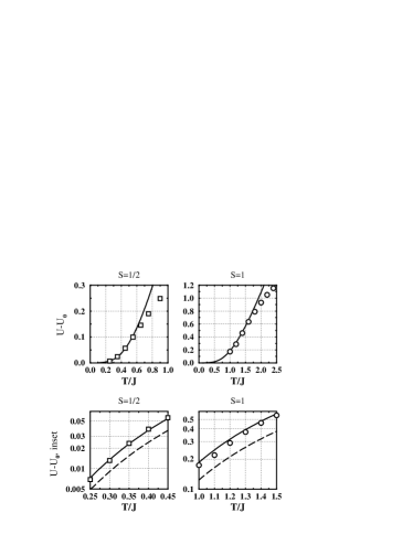
FIG. 1.: Numerical results for the internal energy measured with respect to the ground state $U(T)-U_{0}$ (squares, Ref.[3]; circles, this work) are compared to Eqs.(15-18) without adjustable parameters. Solid line corresponds to $N=3/2$ and dashed line to $N=1$ expected in the renormalized classical regime.

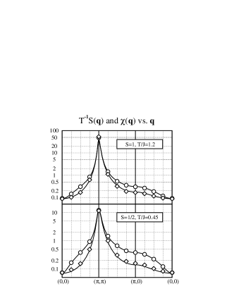
FIG. 2.: Numerical series expansions results for the equal time correlator $T^{-1}S({\bf q})$ (circles) and the static susceptibility $\chi({\bf q})$ (diamonds) across the Brillouin zone are compared to our analytical theory Eqs.(19,20) without adjustable parameters.

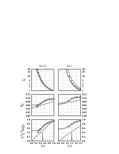
FIG. 3.: Numerical data for the correlation length $\xi$, bulk susceptibility $\chi_{0}$, and normalized Lorentzian amplitude $S_{Q}/(T\xi^{2})$ for $S\!=\!1/2$ and $S\!=\!1$ models, from Ref.[2] (diamonds), Ref.[3] (squares), and this work (circles). Solid lines is the theory presented here; dashed lines is renormalized classical theory [19] with numerical constants calculated in [20, 9]. There are no adjustable parameters; note however that our theoretical curves are completely analytical below the temperature shown by arrow, and use numerically calculated $U(T)$ as input above that temperature.

Comparison With the Numerical Data. The static susceptibility

$$\chi({\bf q},0)=-\frac{4U}{3Z_{\epsilon}^{2}}\times\frac{1}{1+\theta\gamma_{q}}$$ (19)

has exactly the same q-dependence as in the exact solution of the classical Heisenberg chain, and is Lorentzian near the ordering wavevector ${\bf Q}$. Accordingly, the critical dimension of spin in this theory is equal to its mean-field value $\eta=0$. These predictions compare well with the actual nearly Lorentzian shape of $\chi({\bf q},\omega\!=\!0)$ and a very small value of $\eta=0.023$ [21] known from numerical calculations. In contrast with the static susceptibility, the prediction for the equal-time correlator

$$S({\bf q})=-\frac{2}{3}\,U\times\frac{1-\gamma_{q}}{\epsilon_{q}\tanh(\epsilon_{q}/2T)}$$ (20)

does not have Lorentzian shape near ${\bf Q}$. These analytically calculated $\chi({\bf q})$ and $S({\bf q})$ are plotted in Fig.2 as a function of wavevector for the lowest temperature where numerical results for q-dependence are available for comparison. We find good agreement of analytical and numerical curves, achieved without adjustable parameters.

Analytical and numerical results for temperature dependences of the correlation length $\xi(T)=\frac{1}{2}\sqrt{\theta/(1-\theta)}$ (defined from the long-distance decay of correlations $\sim\exp(-R/\xi)$), bulk susceptibility $\chi_{0}(T)$, and normalized Lorentzian amplitude $S_{Q}/(T\xi^{2})$ are plotted in Fig.3. Good agreement between numerical and analytical results is observed in most of the temperature range, except for the lowest temperatures for $S=1/2$ (roughly $\xi>10$) where all three quantities begin to deviate from the theoretical predictions. The deviations are most likely caused by a crossover to the renormalized classical [19] behavior. Evidently, the crossover is completed at still lower temperatures, where no numerical data is currently available; analysis of the experiment remains the only currently available alternative for studying this crossover further.

Summary. We have developed an isotropic spin wave theory of short range magnetic order and compared it with the independently obtained numerical data for $S\!=\!1/2$ and $S\!=\!1$ square lattice antiferromagnets. Unlike the quantum nonlinear sigma or any other continuous model, our theory does not require the correlation length to be much longer than the lattice spacing. Furthermore, because our theory is valid for all wavevectors throughout the Brillouin zone, it is suitable for calculating those quantities that are not dominated by correlations near the ordering wavevector. Its primary drawback, compared to the quantum nonlinear sigma model, is linearity and the resulting lack of mode coupling or dissipation (the continuous limit of our theory is the $O(\infty)$ quantum nonlinear sigma model, and not the physical $O(3)$ model).

We found that the analytical theory agrees with the numerical data without adjustable parameters. In most cases, the agreement is within few per cent in the range of applicability, which for these two models approximately corresponds to the correlation length of less than ten lattice spacings. We expect this theory to be applicable for a variety of other magnets, and are planning to pursue further studies in this direction.

Acknowledgements. We thank R.J. Birgeneau, A.V. Chubukov, M. Greven, T. Jolicoeur, S. Sachdev, S. Sondhi, and O. Starykh for valuable discussions, and A. Sandvik for providing numerical data for comparisons. A.S. is an A.P. Sloan Research Fellow. This work is supported by NSF under Grant No. DMR93-18537, and in part under Grant No. PHY94-07194 through the Institute for Theoretical Physics at UC Santa Barbara. A.S. is grateful to T. Jolicoeur for hospitality during his stay at CEA-Saclay, France, where part of this work was done.

REFERENCES

- [1] Present address (until March 15, 1996): Institute for Theoretical Physics, University of California, Santa Barbara, CA 93106-4030.
- [2] H.-Q. Ding and M.S. Makivic, Phys. Rev. Lett, 64, 1449 (1990); M.S. Makivic and H.-Q. Ding, Phys. Rev. B 43, 3662 (1990).
- [3] A.W. Sandvik and D.J. Scalapino, Phys. Rev. Lett., 72, 277 (1994), and unpublished.
- [4] M. Greven, U.-J. Wiese, and R.J. Birgeneau (unpublished).
- [5] N. Elstner, R. L. Glenister, R. R. P. Singh, and A. Sokol, Phys. Rev. B 51, 8984 (1995).
- [6] B. Keimer et al., Phys. Rev. B 46, (1992) 14034; R.J. Birgeneau et al. (unpublished).
- [7] M. Greven et al., Phys. Rev. Lett. 72, 1096 (1994); Z. Phys. B 96, 465 (1995).
- [8] K. Nakajima et al., Z. Phys. B 96, 479 (1995).
- [9] A.V. Chubukov, S. Sachdev, and J. Ye, Phys. Rev. B 49, 11919 (1994); A.V. Chubukov and S. Sachdev, Phys. Rev. Lett. 71, 169 (1993).
- [10] M.E. Fisher, Am. J. Phys. 32, 343 (1964).
- [11] J. Villain, J. de Physique 35, 27 (1974).
- [12] F.D.M. Haldane, Phys. Lett. 93A, 464 (1983).
- [13] O. Starykh et al., unpublished.
- [14] A. P. Young and B. S. Shastry, J. Phys. C 15, 4547 (1982).
- [15] S.V. Tyablikov, Methods in the Quantum Theory of Magnetism (Plenum Press, New York, NY), 1967.
- [16] P.W. Anderson, Phys. Rev. 86, 694 (1952).
- [17] T. Oguchi, Phys. Rev. 117, 117 (1960).
- [18] J. Igarashi, Phys. Rev. B 46, 10763 (1992).
- [19] S. Chakravarty, B.I. Halperin, and D.R. Nelson, Phys. Rev. B 39, 2344 (1989).
- [20] P. Hasenfratz and F. Niedermayer, Phys. Lett. B 268, 231 (1991); Z. Phys. B 92, 91 (1993).
- [21] C. Holm and W. Janke, preprint; P. Peczak, A.M. Ferrenberg, and D.P. Landau, Phys. Rev. B 43, 6087 (1991).