Incoherent tunnelling through two quantum dots with Coulomb interaction

Abstract

The Ohmic conductance and current through two quantum dots in series is investigated for the case of incoherent tunnelling. A generalised master equation is employed to include the discrete nature of the energy levels. Regions of negative differential conductance can occur in the I-V characteristics. Transport is dominated by matching energy levels, even when they do not occur at the charge degeneracy points.

Due to the improvement of lithographical techniques on a nanometre scale in recent years it has become possible to study systems that were inaccessible to experimentation before. The most easily controlled mesoscopic systems are defined in the 2-dimensional electron gas of a semiconductor. By the application of gate electrodes [2, 3] it is possible to confine the electron gas effectively to produce quantum wires and dots. This allows charge quantisation to be observed in the form of the Coulomb blockade [4, 5]. Moreover, the importance of size quantisation has been shown by Reed et al. who discerned discrete states in small quantum dots [6].

The effect of the charge quantisation has been studied both for a single dot [7] and a double dot [8, 9]. In both cases the level spectrum could be considered continuous. The effect of level quantisation on the Ohmic conductance through a single dot has been studied in the limit of weak coupling to the reservoirs. Coherent [10] and incoherent methods [11] lead to the same result in this limit.

This paper will focus on the transport properties of a double dot with discrete equally spaced energy levels. The limit of completely incoherent tunnelling is studied, where the phase-breaking rate is large and the tunnelling process is sequential. This justifies the use of a semi-classical method like the master equation. It must be noted that the phase-breaking time is still large compared to the time it takes for an electron to traverse the dot. This ensures that the energy levels are quantised, due to the coherence of the wavefunctions inside the dot.

I Generalised master equation

When it is assumed that the tunnelling rates are small compared to the Coulomb energy and the average level spacing, then use of the master equation is justified [12]. In order to take account of the discrete nature of the energy-levels in the dot, the master equation method for dots with a continuous energy level spectrum [7] has to be generalised. The tunnelling rates not only depend on the number of electrons in the dot, but also on their configuration, i.e. how the electrons are distributed over the available energy levels. When there is a high relaxation rate, then the electrons will revert to their local equilibrium distribution between tunnelling events. This is likely to be the case for small tunnelling barriers which cause the electrons to spend a long time in the dot. Since this distribution will depend only on the temperature, the state of the dot may yet again be described simply in terms of the number of electrons present in the dot.

Let $P(p,N)$ be the probability that the system is in a state which is characterised by $N$ electrons in the dot which are distributed over the energy levels according to a configuration $p$. Define $T_{L1}^{pp^{\prime}}(N)$ as the tunnelling rate coefficient corresponding to the transition $\{p,N+1\}\rightarrow\{p^{\prime},N\}$ by an electron tunnelling through the left barrier. $T_{1L}^{p^{\prime}p}(N)$ refers to the rate that corresponds to the reverse process. The tunnelling rates through the right barrier are defined similarly. Finally, there are the relaxation rates $T_{r}^{pp^{\prime}}(N)$ which account for the intra-dot transitions at a fixed electron occupation $N$. The rate of change of the probability of occurrence of the state $\{p,N\}$ is thus given by

$${d\over dt}P(p,N) = \sum_{\Omega=L,R}\sum_{p^{\prime}}\left[T_{\Omega 1}^{p^{\prime}p}(N-1)P(p^{\prime},N-1)+T_{1\Omega}^{p^{\prime}p}(N)P(p^{\prime},N+1)\right]$$ (1)

$$- \sum_{\Omega=L,R}\sum_{p^{\prime}}\left[T_{\Omega 1}^{pp^{\prime}}(N)-T_{1\Omega}^{pp^{\prime}}(N-1)\right]P(p,N)$$ (2)

$$+ \sum_{p^{\prime}}\left[T_{r}^{p^{\prime}p}(N)P(p^{\prime},N)-T_{r}^{pp^{\prime}}(N)P(p,N)\right]$$ (3)

If the system consists of several dots in series, it is necessary to define the tunnelling rates between the dots. Define $T_{i,i\pm 1}^{pp^{\prime},qq^{\prime}}(N_{i},N_{i\pm 1})$ as the tunnelling rate corresponding to the transition $\{p,N_{i}+1\}\rightarrow\{p^{\prime},N_{i}\}$ and $\{q,N_{i\pm 1}\}\rightarrow\{q^{\prime},N_{i\pm 1}+1\}$ where the subscript $i$ labels the site of the dot. The evolution of the multi-particle state occupation probabilities for a dot not neighboured by a reservoir is given by

$${d\over dt}P(p,N_{i}) = \sum_{N_{i\pm 1}}\sum_{p^{\prime},q,q^{\prime}}T_{i,i\pm 1}^{p^{\prime}p,qq^{\prime}}(N_{i},N_{i\pm 1})P_{i}(p^{\prime},N_{i}+1)P_{i\pm 1}(q,N_{i\pm 1})$$ (4)

$$+ \sum_{N_{i\pm 1}}\sum_{p^{\prime},q,q^{\prime}}T_{i\pm 1,i}^{qq^{\prime},p^{\prime}p}(N_{i\pm 1},N_{i}-1)P_{i}(p^{\prime},N_{i}-1)P_{i\pm 1}(q,N_{i\pm 1}+1)$$ (5)

$$- \sum_{N_{i\pm 1}}\sum_{p^{\prime},q,q^{\prime}}T_{i,i\pm 1}^{pp^{\prime},qq^{\prime}}(N_{i}-1,N_{i\pm 1})P_{i}(p,N_{i})P_{i\pm 1}(q,N_{i\pm 1})$$ (6)

$$- \sum_{N_{i\pm 1}}\sum_{p^{\prime},q,q^{\prime}}T_{i\pm 1,i}^{qq^{\prime},pp^{\prime}}(N_{i\pm 1},N_{i})P_{i}(p,N_{i})P_{i\pm 1}(q,N_{i\pm 1}+1)$$ (7)

$$+ \sum_{p^{\prime}}\left[T_{r}^{p^{\prime}p}(N)P_{i}(p^{\prime},N)-T_{r}^{pp^{\prime}}(N)P_{i}(p,N)\right]$$ (8)

For both the single and the multiple dot system the steady state current can be written as

$$J=e\sum_{p,p^{\prime}}\sum_{N}\left[T_{L1}^{pp^{\prime}}(N)P(p,N)-T_{1L}^{p^{\prime}p}P(p^{\prime},N)\right]$$ (9)

When it is assumed that the relaxation rates are large compared to the tunnelling rates, then the number of electrons in the dots is the only significant variable, since knowledge of this quantity allows one to deduce the probabilities of the various electronic configurations. Hence the formalism is greatly simplified. However, the tunnelling rates between states with a different occupation number have to be redefined to include the weighted sum over all possible tunnelling paths. Define $T_{L1}(N)$ and $T_{1L}(N)$ as the tunnelling rates for an electron tunnelling into and out of the dot through the left barrier with $N$ other electrons present in the dot.

$$T_{L1}(N) = \sum_{p,p^{\prime}}T_{L1}^{pp^{\prime}}(N)P(p|N)$$ (10)

$$T_{1L}(N) = \sum_{p.p^{\prime}}T_{1L}^{pp^{\prime}}(N)P(p|N+1)$$ (11)

where $P(p|N)$ is the conditional probability that the system is in configuration $p$ given that there are $N$ electrons in the dot. Since the master equation takes only single electron tunnelling events into consideration, the only contributions that need to be taken into account are those where $p$ and $p^{\prime}$ differ by the occupation of one energy level. Therefore the double sum over $p$ and $p^{\prime}$ can be replaced by a single sum over the single particle energy levels $k$.

$$T_{L1}(N) = \sum_{k}T_{L1}^{k}(N)[1-P(k|N)]$$ (12)

$$T_{1L}(N) = \sum_{k}T_{1L}^{k}(N)P(k|N)$$ (13)

Here $P(k|N)$ is the conditional probability that level $k$ is occupied given that there are $N$ electrons in the dot. For inter-dot tunnelling events the rates are re-expressed in terms of a sum over the tunnelling paths from all levels $k$ in dot $i$ to all levels $l$ in dot $i\pm 1$

$$T_{i,i\pm 1}(N_{i},N_{i\pm 1})=\sum_{k,l}T_{i,i\pm 1}^{k,l}(N_{i},N_{i\pm 1})P_{i}(k|N_{i}+1)[1-P_{i\pm 1}(l|N_{i\pm 1})]$$ (14)

For the case of negligible energy level broadening the probability $P_{i}(k|N_{i})$ of finding an electron on level $k$ of dot $i$ given $N_{i}$ electrons can be determined from the Boltzmann distribution.

$$P_{i}(k|N_{i}) = e^{-\beta\epsilon_{k}(N_{i}-1)}{Z_{i}^{k}(N_{i}-1)\over Z_{i}(N_{i})}$$ (15)

$$1-P_{i}(k|N_{i}) = {Z_{i}^{k}(N_{i})\over Z_{i}(N_{i})}$$ (16)

where $\beta=1/k_{B}T$ and $\epsilon_{k}(N_{i}-1)$ is the energy required to add an electron at an energy level $k$ when $N_{i}-1$ electrons are already present in the dot. $Z_{i}(N_{i})$ is the partition function for $N_{i}$ electrons in dot $i$, $Z_{i}^{k}(N_{i})$ is the conditional partition function for $N_{i}$ electrons given that level $k$ is unoccupied. When the conditional probabilities are substituted in equation 14, one obtains

$$T_{i,i\pm 1}(N_{i},N_{i\pm 1})=\sum_{k,l}{e^{-\beta\epsilon_{k}(N_{i})}Z_{i}^{k}(N_{i})Z_{i\pm 1}^{l}(N_{i\pm 1})\over Z_{i}(N_{i})Z_{i\pm 1}(N_{i\pm 1})}T_{i,i\pm 1}^{k,l}(N_{i},N_{i\pm 1})$$ (17)

Tunnelling events between dots will in general not preserve energy, since it is unlikely that energy levels will line up. The high relaxation rate suggests that all tunnelling events can be considered inelastic. Hence

$$T_{i\pm 1,i}^{l,k}(N_{i\pm 1},N_{i})=e^{-\beta[\epsilon_{l}(N_{i\pm 1})-\epsilon_{k}(N_{i})]}T_{i,i\pm 1}^{k,l}(N_{i},N_{i\pm 1})$$ (18)

It follows from the two preceding equations that the tunnelling rates are inelastic in the total free energy of the system. This is also true for tunnelling between dot and reservoir. This implies that the following condition holds true at zero bias for $\cal N$ dots for all possible occupation numbers $N_{i}$.

$$T_{L1}\left(\prod_{i=1}^{{\cal N}-1}T_{i,i+1}\right)T_{{\cal N}R}=T_{R{\cal N}}\left(\prod_{i=1}^{{\cal N}-1}T_{i+1,i}\right)T_{1L}$$ (19)

II The canonical distribution

One of the quantities that is needed to calculate the tunnelling rate between dots of specified occupation number is the probability $P(k|N)$ that an energy level $k$ is occupied given a total occupation of $N$ electrons. When no relaxation of the electrons in the dot is allowed the occupation of the levels will be determined by the coupling to the reservoirs. However, in the presence of thermalisation the levels will be filled according to some equilibrium distribution independent of the energies at which the electrons initially entered the dot. In metals the energy-levels are filled according to the Fermi-Dirac distribution function. Naively one might expect this also to hold for discrete energy levels and this has been assumed in various papers. Unfortunately, this is not generally the case. In metallic systems the levels are very closely spaced so that the addition of an additional electron will have no effect on the distribution, whereas this is not true for a discrete level spectrum. In this section the correct distribution will be calculated for a dot with an infinite number of equally spaced energy levels, containing $N$ electrons. The calculation is done for energy levels with negligible broadening ($\Gamma\ll k_{B}T$).

Consider the partition function $Z(N)$ for a dot containing $N$ electrons, with energy levels $\epsilon_{k}=\epsilon_{0}+k\Delta_{\epsilon}$.

$$Z(N)=\sum_{p\{N\}}e^{-\beta(n_{1}\epsilon_{1}+n_{2}\epsilon_{2}+...)}$$ (20)

where the sum is taken over all realisations $p\{N\}$ with $N=\sum_{k}n_{k}$. Explicitly expand out the contribution of the lowest energy level (either $n_{1}=1$ or $n_{1}=0$).

$$Z(N)=e^{-\beta\epsilon_{1}}\sum_{p\{N-1\}}e^{-\beta(n_{2}\epsilon_{2}+n_{3}\epsilon_{3}+...)}+\sum_{p\{N\}}e^{-\beta(n_{2}\epsilon_{2}+n_{3}\epsilon_{3}+...)}$$ (21)

When it is assumed that there is an infinite number of energy levels, then the sum over the occupation numbers $n_{k}$ ($k>1$) can be transformed to the partition function over all levels (including $k=1$). Rewriting $\epsilon_{k}=\epsilon_{k-1}+\Delta_{\epsilon}$ and relabelling $n_{k}\rightarrow n_{k-1}$, the following recursion relation is obtained.

$$(1-e^{-\beta N\Delta_{\epsilon}})Z(N)=e^{-\beta\epsilon_{0}}e^{-\beta N\Delta_{\epsilon}}Z(N-1)$$ (22)

With the boundary condition given by $Z(0)=1$, this is solved to give

$$Z(N)=e^{-\beta N\epsilon_{0}}\prod_{n=1}^{N}\left({1\over e^{\beta n\Delta_{\epsilon}}-1}\right)$$ (23)

This expression for the partition function does not explicitly include the many-body interaction. This is irrelevant in this context, since the number of electrons is kept constant. However, when one wants to calculate the probability that the dot contains a certain number of electrons, the Coulomb interaction obviously needs to be included. For a simple model of the interaction where all pairs of electrons have an associated Coulomb repulsion $U$, the full interactive partition function is obtained by multiplication with a factor $\exp[-\beta N(N-1)U/2]$.

Now it is possible to do a similar calculation to obtain an expression for $Z^{k}(N)$, the conditional partition function for $N$ electrons given that level $k$ is unoccupied. However, in contrast to the full partition function, this requires one to solve a recursion relation in both parameters $k$ and $N$. This can be avoided by using equations 15 and 16 to yield a recursion relation of the conditional probability $P(k|N)$ directly.

$$P(k|N)=e^{-\beta\epsilon_{0}}e^{-\beta\Delta_{\epsilon}k}{Z(N-1)\over Z(N)}\left[1-P(k|N-1)\right]$$ (24)

Since the full partition functions are known, this is easily solved to give

$$P(k|N)=\sum_{q=1}^{N}(-1)^{q-1}\prod_{p=1}^{q}e^{-\beta\Delta_{\epsilon}k}\left(e^{\beta\Delta_{\epsilon}(N+1-p)}-1\right)$$ (25)

In order to compare this with the Fermi-Dirac distribution function, one needs to consider a very large number of electrons in the dot. The occupation probability will depend only on the difference $x=k-N-1/2$.

$$P_{\infty}(x)=\sum_{q=1}^{\infty}(-1)^{q-1}e^{-\beta\Delta_{\epsilon}q(x+q/2)}$$ (26)

For computational reasons the above equation is rewritten as

$$P_{\infty}(x)=2e^{{\beta\Delta_{\epsilon}\over 2}(x^{2}-1/4)}\left\{\begin{array}[]{ll}\sum_{q=0}^{\infty}e^{-2\beta\Delta_{\epsilon}(q-x/2+1/4)^{2}}\sinh\left[\beta\Delta_{\epsilon}(q-x/2+1/4)\right]&x<0\\ \sum_{q=0}^{\infty}e^{-2\beta\Delta_{\epsilon}(q+x/2+3/4)^{2}}\sinh\left[\beta\Delta_{\epsilon}(q+x/2+3/4)\right]&x>0\end{array}\right.$$ (27)

The distribution function has been plotted in figure 1 for various values of $\beta\Delta_{\epsilon}$. In the metallic limit, when the level spacing is small compared to the temperature, the distribution tends towards the Fermi-Dirac distribution function, as expected. When the temperature is comparable or smaller than the level spacing, the distribution deviates significantly. Its limiting behaviour is well described by another Fermi-Dirac distribution function with an effective temperature which is half the real temperature. A slightly more accurate result for the occupation probability in the limit $\beta\Delta_{\epsilon}\gg 1$ is given by (note that $x\neq 0$ by definition)

$$P_{\infty}(x)=\left\{\begin{array}[]{ll}{1\over e^{\beta\Delta_{\epsilon}(x-1/2)}+1}&x<0\\ {1\over e^{\beta\Delta_{\epsilon}(x+1/2)}+1}&x>0\end{array}\right.$$ (28)

III Tunnelling through a single dot

When the energy level broadening is negligible compared to the temperature, i.e. in the limit of weak coupling to the reservoirs, the density of states in the dot can be adequately described by a set of delta functions. The leads are assumed to be in thermal equilibrium, described by the Fermi-Dirac distributions $f_{L}$ and $f_{R}$. To a first approximation, the electron-electron interaction can satisfactorily be described using the charging model, where each pair of electrons has an associated Coulomb repulsion of $U$. Fermi’s golden rule gives the tunnelling rates between the dot and the reservoirs for all energy levels $k$.

$$T_{L1}^{k}(N) = {\Gamma_{L}\over\hbar}f_{L}(\epsilon_{k}+NU)$$ (29)

$$T_{1L}^{k}(N) = {\Gamma_{L}\over\hbar}[1-f_{L}(\epsilon_{k}+NU)]$$ (30)

where $\Gamma_{L}=2\pi\rho_{L}|V_{L}|^{2}$ is the strength of coupling to the left reservoir. The expressions for the tunnelling rates through the right barrier are similar. It is assumed that the quantum dot can be approximated by a parabolic confining potential so that the single particle energy levels are equally spaced by an energy $\Delta_{\epsilon}$. In figures 2 and 3 the current and its associated differential conductance is plotted as a function of the applied bias for a range of energy level spacings. In numerical calculations it is possible to take into account more realistic energy level spectra, enabling a closer comparison with experiment. When it is taken into account that the total spin of the system can only change by $1/2$ with each tunnelling event, it appears that negative differential conductance may occur in specific regions [13, 14].

In general a dot with closely packed energy levels yields a higher current than a dot with a sparse energy level spectrum, because of the higher number of current paths available. When $\Delta_{\epsilon}\ll U$ then the metallic regime is entered.

When the energy level spacing is not negligible, the I-V characteristics are typified by two energy scales, the Coulomb repulsion energy $U$ and the bare energy level spacing $\Delta_{\epsilon}$. As in the metallic regime, one expects the I-V characteristic to display a current step whenever the maximum occupation of the dot increases by one. This happens with a period $U+\Delta_{\epsilon}$, since an extra electron not only has to overcome the Coulomb barrier but also has to tunnel to the next available energy level. In addition, there is also some fine structure which has an associated period of $\Delta_{\epsilon}$. This is caused by the fact that an extra current path is created when the bias is increased by $\Delta_{\epsilon}$.

When $\Gamma_{L}\gg\Gamma_{R}$ the dot will be mostly maximally occupied and the most marked current increases occur whenever the Coulomb blockade can be overcome. This means that the period $U+\Delta_{\epsilon}$ is accentuated. In the opposite regime $\Gamma_{L}\ll\Gamma_{R}$ the dominant period is the level spacing. Under normal operating conditions $\Gamma_{L}\simeq\Gamma_{R}$ the two periods coexist (see figure 3). It is noted that at higher bias voltages the number of peaks in the differential conductance increases, as new current paths become available at different energies for different occupation numbers. Only when the ratio $U/\Delta_{\epsilon}$ is an integer do peaks corresponding to different occupation numbers coincide.

The Ohmic conductance through a quantum dot (figure 4) differs from that through a metallic dot in two significant ways. Firstly, the periodicity of the conductance peaks has increased by the level spacing $\Delta_{\epsilon}$. Secondly, the temperature dependence of the peaks has changed its nature. An increase in temperature now not only leads to larger thermal broadening, but also to a lowering of the peak amplitude which is inversely proportional to the temperature. This is due to the fact that transport proceeds through a single energy level. The temperature dependence is proportional to the derivative of the Fermi-distribution function in the reservoirs [15]. Therefore, at low temperatures $k_{B}T\ll U$ the Ohmic conductance can be written as

$$G(\mu)={e^{2}\over\hbar}{\Gamma_{L}\Gamma_{R}\over\Gamma_{L}+\Gamma_{R}}\sum_{N}{1\over 4k_{B}T\cosh^{2}({\mu-\mu_{N}\over 2k_{B}T})}$$ (31)

where the successive charge degeneracy points $\mu_{N}$ are spaced by an energy $U+\Delta_{\epsilon}$. For higher temperatures several levels should be taken into consideration, each of which is weighted by a factor determined by the Boltzmann distribution [11].

$$G(\mu)={e^{2}\over\hbar}{\Gamma_{L}\Gamma_{R}\over\Gamma_{L}+\Gamma_{R}}\sum_{N}\sum_{i}{1\over k_{B}T}P_{i}(N)f\left({\epsilon_{i}+NU-\mu\over 2k_{B}T}\right)$$ (32)

where $P_{i}(N)$ is the joint probability that the dot contains $N$ electrons and that the single particle level $\epsilon_{i}$ is empty. Note that the contributions from levels other than at positions $\mu_{N}$ are too small to cause a peak in the conductance.

Apart from the I-V characteristics and the Ohmic conductance, there is a third useful experiment that can be carried out. This involves applying a constant bias across the dot and studying the resultant current as a function of the gate potential. Typically the source-drain bias is chosen to be less than the charging energy which isolates the effects of the energy separation of the zero dimensional states of the dot. In figure 5 the current has been calculated as a function of the gate voltage for a dot with a constant level spacing $\Delta_{\epsilon}=0.1U$. The thermal energy is given by $k_{B}T=0.01U$. In accordance with some recent experiments [16, 17, 18] a number of peaks and troughs can be observed in the current. All peaks and troughs can be characterised by the number of levels available to an incoming electron to tunnel onto, and the number of levels from which an electron can tunnel out of the dot. For a Fermi level separation $\delta\mu$ of $0.15U$ between the reservoirs (see figure 5) these numbers are $1,2\rightarrow 1,1\rightarrow 2,1$. This explains why the total peak is split into two subpeaks. For the second set of graphs with $\delta\mu=0.27U$ the sequence of available tunnelling levels is $1,3\rightarrow 1,2\rightarrow 2,2\rightarrow 2,1\rightarrow 3,1$. It is also clear that asymmetric tunnelling barriers cause the current peaks to be asymmetric.

IV Tunnelling through two dots in series

When studying the current and conductance properties of two quantum dots connected in series between the source and the drain, one obviously has to take into account the tunnelling between the dots. Inter-dot transitions are qualitatively different from transitions between a dot and a reservoir. The reservoir can be assumed to have a continuous density of states, so that electrons can always tunnel elastically into and out of the reservoir. Even though inelastic tunnelling events would in principle be allowed, their contribution would be relatively small compared to the elastic tunnelling rate. Therefore inelastic scattering only has a significant effect on the transport through a single dot if the scattering takes place inside the dot, i.e. relaxation.

As far as tunnelling between dots is concerned, it is clear that the elastic tunnelling rate is significant only when the energy levels in the dots line up. This is obviously not generally the case. Usually an electron would have to interact inelastically in order to tunnel to a different energy level in the neighbouring dot. The energy difference would normally be absorbed or provided by phonons.

As a theoretical model, one can consider the double dot system to be coupled to a phonon reservoir or a heat bath with a coupling strength $|V_{ph}|^{2}$. The energy spectrum of the independent oscillators of the phonon reservoir is characterised by the density of phonon states $\rho_{ph}(E)$. Some work has been done to calculate the current through a double-barrier resonant structure with some interaction between electrons and photons [19, 20, 21]. The coupling to the optical phonons creates transmission subbands which are observable in the I-V characteristics. In this section, where inter-dot transmission is considered, the interaction with acoustic phonons will be the dominant mechanism. The energy spectrum for acoustic phonons is given by the Debye density of states.

$$\rho_{ph}(E)=C_{ph}\left\{\begin{array}[]{ll}E^{2}&E<k_{B}\Theta_{D}\\ 0&E>k_{B}\Theta_{D}\end{array}\right.$$ (33)

In a two-dimensional electron gas the Debye temperature $\Theta_{D}$ is approximately in the range $\Theta_{D}\sim 200-700K$ [22]. This is of the order of a few tens of $meV$, which corresponds to several times the Coulomb interaction energy $U$. This is typically larger than the voltage drop across the device, so that one can simply use the phonon density of states below the cut-off energy $k_{B}\Theta_{D}$.

Phonons are bosons, so that the Pauli principle does not apply and states can be multiply occupied. The average occupation number of states at a given energy is given by the Bose-Einstein distribution $n_{B}(E)$.

$$n_{B}(E)={\Theta(E)-\Theta(-E)\over e^{E/k_{B}T}-1}$$ (34)

where $\Theta(E)$ is the Heaviside step function and $E$($-E$) is the energy provided (absorbed) by the phonon bath. The Bose-Einstein distribution at positive and negative values of $E$ differs by $1$, which is indicative of the fact that a heat bath can always absorb energy.

A plausible model for the inelastic tunnelling rate $T_{12}^{kl}$ between an energy level $\epsilon_{k}$ in the first dot and $\epsilon_{l}$ in the second dot is as follows

$$T_{12}^{kl}={|V_{ph}|^{2}\over\hbar}\int_{-\infty}^{\infty}d\omega\int_{-\infty}^{\infty}d\omega^{\prime}\rho_{1}^{k}(\omega)\rho_{2}^{l}(\omega^{\prime})\left[\sum_{1,2}|\phi^{k}(\omega)\phi^{l}(\omega^{\prime})|^{2}\right]\rho_{ph}(\omega^{\prime}-\omega)n_{B}(\omega^{\prime}-\omega)$$ (35)

where $\rho_{1}^{k}(\omega)$ and $\rho_{2}^{l}(\omega^{\prime})$ are the densities of state for the energy levels. Considering the dots in isolation from the reservoirs, the eigenstates cannot be regarded as localised in each of the dots, but the wavefunctions will leak slightly into the other dot by virtue of the hopping potential $V_{M}$. This results in the overlap integrals $|\phi_{1}^{k}(\omega)\phi_{1}^{l}(\omega^{\prime})|^{2}$ and $|\phi_{2}^{k}(\omega)\phi_{2}^{l}(\omega^{\prime})|^{2}$. Naively this can be interpreted as the probability that the inelastic process can take place between the wavefunction components in the same dot. The wavefunctions are calculated from a simple two-dimensional Hamiltonian with diagonal elements $\omega$ and $\omega^{\prime}$ and off-diagonal elements given by the hopping potential $V_{M}$. By calculating its eigenvectors the overlap matrix can be determined.

$$\sum_{1,2}|\phi^{k}(\omega)\phi^{l}(\omega^{\prime})|^{2}={2V_{M}^{2}\over(\omega^{\prime}-\omega)^{2}+4V_{M}^{2}}$$ (36)

The density of states in the dots is broadened mainly as a result of the inelastic scattering, which is a prerequisite for the incoherent regime. To a first approximation the broadening can be considered as a Lorentzian distribution [23] with a broadening $\Gamma_{\phi}$ proportional to the phase-breaking rate. Now equation 35 can be rewritten as a single integral over the energy difference $E=\omega^{\prime}-\omega$ between the initial and final state.

$$T_{12}^{kl}=A_{ph}\int_{-\infty}^{\infty}dE{\Gamma_{\phi}/\pi\over(E+\epsilon_{k}-\epsilon_{l})^{2}+\Gamma_{\phi}^{2}}{E^{2}\over E^{2}+4V_{M}^{2}}n_{B}(E)$$ (37)

with $A_{ph}=2V_{M}^{2}|V_{ph}|^{2}C_{ph}/\hbar$.

It must be stressed that the broadening of the energy levels should be much less than the temperature. Otherwise it is not valid anymore to use the Boltzmann distribution to calculate the occupation probabilities. This assumption is consistent with the calculation of the reservoir-dot transition rate of section III. Figure 6a shows the energy dependence of the inter-dot tunnelling rate for the case when the energy-levels are considered to be $\delta$-functions. However, it should still be taken into account that the level broadening is large compared to the coupling between the dots, causing the peaks in the transition rate at $E=\pm 2V_{M}$ to be smeared. At energy differences $\Delta=\epsilon_{l}-\epsilon_{k}$ which are small compared to the broadening, the transition rate can now be approximated by a Lorentzian of width $2\Gamma_{\phi}/\hbar$ and height $2A_{ph}{\rm ln}[\Gamma_{\phi}/2V_{M}]/\pi\Gamma_{\phi}$ (see figure 6b). At larger energy differences $|\Delta|>\Gamma$ the function is sufficiently close to the Bose-Einstein distribution.

As the broadening is much smaller than the thermal energy, the inter-dot transition rate for small $\Delta$ can get much larger than the transition rate between dot and reservoir so that the inter-dot transition is no longer the current-limiting process. In this case it is of no relevance whether the transition rate between the dots is infinite or simply very large. This suggests that the inter-dot transition rate may be approximated by the Bose-Einstein distribution $A_{ph}n_{B}(\Delta)$ at all values of $\Delta$. This makes the mathematical analysis much more transparent.

When one calculates the transition rate between dots with a given occupation number, one should sum over all possible tunnelling events according to equation 14. The greatest contribution should come from the energy range where the electron can tunnel from levels which are mostly occupied to levels which are mostly empty. Outside this window the product $P_{1}(k|N_{1}+1)[1-P_{2}(l|N_{2})]$ falls off exponentially. However, since the Bose-Einstein distribution diverges at $\Delta\rightarrow 0$, the total transition rate seems to be dominated by matching levels, even when they are situated at energies far removed from the Fermi level. This is clearly an unphysical situation. This anomaly can be removed by again including the broadening in the calculation of the transition rate. Alternatively, it can be argued that the transition rate for a given pair of levels is the combination of the previously defined rate and the rate at which electrons can get into an excited level. This second rate is the relaxation rate $\hbar/\tau_{\rm rel}$. Remembering that the inverses of the rates of consecutive processes add together, the total inter-dot rate can be obtained for given occupation numbers.

$$T_{12}(N_{1},N_{2})=\sum_{k,l}P_{i}(k|N_{i}+1)[1-P_{i\pm 1}(l|N_{i\pm 1})]{T_{12}^{kl}\hbar/\tau_{\rm rel}\over T_{12}^{kl}+\hbar/\tau_{\rm rel}}$$ (38)

In order to perform some realistic simulations it is helpful to know the dependence on the size of both the charging energy $U$ and the confinement energy $\Delta_{\epsilon}$. In the charging model approximation the Coulomb repulsion is inversely proportional to the capacitance $C$ of the dot. This implies that the repulsion energy $U$ is also inversely proportional to the area of the dot. The single particle energy level spacing is given by [24]

$$\Delta_{\epsilon}={\pi\hbar^{2}\over m^{*}{\rm area}}$$ (39)

where $m^{*}$ is the effective mass of an electron in the two dimensional electron gas in which the quantum dot has been defined. It follows that both the Coulomb energy and the level spacing scale inversely proportionally to the area of the quantum dot.

A Ohmic conductance

Figure 7 shows the Ohmic conductance through two dots with a relatively strong inelastic tunnelling coefficient $A_{ph}$. In order to analyse the structure of the peaks, assume that the total occupancy of each dot can only fluctuate by one electron. Moreover, assume that only a single level per dot (at the charge degeneracy points) contributes substantially to the transport. Then the global master equation is used to obtain an expression for the Ohmic conductance.

$$G = {e^{2}A_{ph}\Gamma_{L}\Gamma_{R}(\Gamma_{L}+\Gamma_{R})\over 4k_{B}T\cosh\left({\mu-\epsilon_{k}\over 2k_{B}T}\right)\cosh\left({\mu-\epsilon_{l}\over 2k_{B}T}\right)}\times\left[A_{ph}\hbar\left({\Gamma_{L}^{2}\cosh\left({\mu-\epsilon_{l}\over 2k_{B}T}\right)\over\cosh\left({\mu-\epsilon_{k}\over 2k_{B}T}\right)}+{\Gamma_{R}^{2}\cosh\left({\mu-\epsilon_{k}\over 2k_{B}T}\right)\over\cosh\left({\mu-\epsilon_{l}\over 2k_{B}T}\right)}\right)\right.$$ (40)

$$+ \left.2A_{ph}\hbar\Gamma_{L}\Gamma_{R}\cosh\left({\epsilon_{k}-\epsilon_{l}\over 2k_{B}T}\right)+2\Gamma_{L}\Gamma_{R}(\Gamma_{L}+\Gamma_{R})\sinh\left({|\epsilon_{k}-\epsilon_{l}|\over 2k_{B}T}\right)\right]^{-1}$$ (41)

When the two reservoirs are equally strongly coupled to the dots, i.e. $\Gamma_{L}=\Gamma_{R}=\Gamma$, then the above expression peaks at $\mu=(\epsilon_{k}+\epsilon_{l})/2$. The peak conductance is given by (using $\Delta=\epsilon_{l}-\epsilon_{k}$)

$$G_{\rm max}={e^{2}A_{ph}\Gamma\over 8k_{B}T\cosh^{3}\left({\Delta\over 4k_{B}T}\right)\left[A_{ph}\hbar\cosh\left({\Delta\over 4k_{B}T}\right)+2\Gamma\sinh\left({|\Delta|\over 4k_{B}T}\right)\right]}$$ (42)

When the peak height is investigated as a function of the temperature, then it appears that it has a maximum at a value of $k_{B}T/|\Delta|$ which is given by the solution of the following transcendental equation.

$$\left(2{A_{ph}\hbar\over\Gamma}{|\Delta|\over k_{B}T}+3{|\Delta|\over k_{B}T}-4\right)\tanh\left({|\Delta|\over 4k_{B}T}\right)=2{A_{ph}\over\Gamma}-{|\Delta|\over k_{B}T}$$ (43)

The solution is plotted in figure 8. When the ratio of the inelastic tunnelling coefficient to the reservoir coupling $A_{ph}\hbar/\Gamma$ is of order unity or larger, then the temperature at which a particular conductance peak reaches its maximum height is given by roughly half the energy difference $|\Delta|$. This maximum height is larger as the energy difference $\Delta$ gets smaller. This calculation is in good quantitative agreement with the temperature dependence of the conductance curves of figure 7. At higher temperatures the calculation becomes more inaccurate as several levels and more occupation numbers will start to contribute to the transport.

In figure 9 the conductance is shown for a double dot system which is identical to that of figure 7 with the exception that the inelastic tunnelling coefficient is two orders of magnitude smaller. From figure 8 one would expect the peaks to be maximised at a temperature $k_{B}T\simeq 2.2|\Delta|$. The above description of the conductance peaks seems to apply to most of the peaks. However, it is clear that the peak which is situated at $\mu\simeq-4.7U$ has an anomalous behaviour. The conductance at this point is much larger than expected. This is due to the fact that one of the lower levels in the first dot very nearly matches up with the dominant level in the second dot, thus strongly enhancing the inter-dot tunnelling rate.

This effect most strongly shows up when the inelastic tunnelling coefficient $A_{ph}\hbar$ is small compared to the coupling $\Gamma$ to the reservoirs. This is simply due to the fact that the inter-dot tunnelling is the main current-limiting process and will therefore tend to dominate the physics. For large inelastic tunnelling coefficients the current will mainly be determined by the matching of the levels between dot and reservoir. This explains why the afore-mentioned effect is almost imperceptible in figure 7.

B Current characteristics

The current-voltage characteristics have been calculated in figure 10 for a double dot system with specifications as indicated in the caption. Figure 11 shows the results for a system where the dot specifications have been swapped. Physically this simply amounts to varying the chemical potential in the right reservoir instead of the left reservoir.

At low temperatures two periods may be observed in the I-V characteristics. The larger period is given by the Coulomb repulsion in the first dot plus a single particle spacing $U_{1}+\Delta_{\epsilon_{1}}$. The smaller period is simply given by the single particle spacing $\Delta_{\epsilon_{1}}$. This behaviour is reminiscent of the current through a single dot with $\Gamma_{L}\gg\Gamma_{R}$ (see section III). In other words, the second dot with its surrounding barriers acts as a single barrier with a reduced transparency. The electrons which have entered the first dot will tunnel into a lower energy level in the second dot at a rate of approximately $A_{ph}$ since the levels in the dots will not normally line up. At larger temperatures the current curves will lose some features due to thermal smearing. This is clearly the case in figure 11.

However, the current curve of figure 10 has a more complicated form at high temperatures. It has a region of negative differential conductance which occurs in the bias range where the average occupancy of the first dot increases from one to two electrons with respect to the average occupation number at zero bias. This can be explained by considering the (unlikely) case where a pair of energy levels matches up for a given set of occupation numbers. This will result in a highly increased tunnelling rate between the dots. When the bias across the device is raised the average occupancy of the dot will increase. This means that the dots are less likely to contain the number of electrons for which the levels lined up. Consequently the tunnelling rate between the dots and hence the overall current will decrease, in spite of the fact that the total number of tunnelling paths is likely to have increased.

The temperature at which negative differential conductance can occur (if at all) is set by the energy difference of the matching pair of levels in the dots. Their energy separation has to be significantly less than $k_{B}T$ for the tunnelling rate to increase dramatically. A higher temperature can cause some levels to match up which could not really be considered energetically close at lower temperatures. However, a higher temperature also means that there is a smaller probability that the total inter-dot tunnelling is dominated by just a single pair of levels. This will reduce the effect. The conclusion is that negative differential conductance is more likely to occur at higher temperatures, but when it occurs at a lower temperature the effect will be more pronounced.

Similar to the one dot case, one can extract information about the level spacing when one considers the current through the system at fixed bias $\delta\mu$ while varying the gate voltage of one of the dots, a measurement first performed by van der Vaart et al. [25]. This is depicted in figure 12. The Coulomb repulsion energies and the level spacings are the same as before. The inelastic tunnelling coefficient is small compared to the dot-reservoir coupling. The empty levels are the levels that an excess electron can occupy. Note that no more than a single extra electron can be contained in the dot, since this is prevented by the Coulomb blockade. Since electrons carry a negative charge, a rise in the gate potential causes a downward shift of the energy levels.

The results are shown in figure 13 for a range of values of $\delta\mu$. A few generic features can be noted which are also true for tunnelling through a single dot. Firstly, the current is periodic in the gate voltage with a period $U_{1}+\Delta_{\epsilon_{1}}$. Only a single period is shown in the figure. Secondly, a significant current is only allowed to flow when the Coulomb blockade is overcome in both dots. This requires the lowest available level in each dot to lie within the energy window $\delta\mu$. This is clearly shown in figure 13 where a larger bias voltage allows the current to flow at more values of the gate potential.

The most striking feature of figure 13 is the occurrence of sharp current peaks. These happen at values of the gate voltage where one of the occupied states of the first dot (containing the excess electron) lines up with an empty level in the second dot. It is clear that this will happen with a periodicity $\Delta_{\epsilon_{1}}$ (in the figure $\Delta_{\epsilon_{1}}=0.13U$). When the bias voltage is such that several levels in the second dot are contained within the energy window $\delta\mu$, then peaks will also occur at intervals $\Delta_{\epsilon_{2}}$. This is the case in the third graph of figure 13, where $\Delta_{\epsilon_{2}}=0.32U$.

Finally, note that the current in the valleys between the peaks increases more or less linearly with the number of peaks. This reflects the fact that at a higher gate potential there are more electrons in the first dot which are able to tunnel downwards in energy into the second dot. Each tunnelling path has an associated off-resonance tunnelling rate of $A_{ph}$ which will contribute an amount $A_{ph}\hbar I_{0}/\Gamma$ towards the total current (assuming $A_{ph}\hbar\ll\Gamma$). Therefore the current minima should increase by this amount every time the gate potential is increased by an amount $\Delta_{\epsilon_{1}}$.

This seems to be a much more powerful method for determining the single particle level spacing than the analogous experiment with a single dot. In the model used in this chapter, the line shape will be a multiple of the Bose-Einstein distribution. However, at very small energy separations $\Delta$ the intrinsic width of the levels becomes significant and the lineshape will be approximately a Lorentzian of width $2\Gamma_{\phi}$ near resonance but will be asymmetric off-resonance. This seems to corresponds at least qualitatively to recent experiment [25]. In the case of large $A_{\rm ph}\hbar/\Gamma$, the middle barrier is no longer the current limiting barrier and the current will not peak anymore but simply increase with $\Delta$ until a saturation value of ${2\over 3}e^{2}/\hbar$ is reached. Further experiments will have to show whether it is justified to assume that the inelastic tunnelling rate can be approximated by the Bose-Einstein distribution. If this turns out to be a false assumption, then the master equation can still be used to model the effect of a more realistic inelastic tunnelling rate.

V Conclusions

For a dot with discrete levels, the distribution function at equilibrium differs from the Fermi-Dirac distribution, especially at low temperatures. The peaks in the Ohmic conductance are spaced by an amount $U+\Delta_{e}$. In the I-V characteristics the effect of both the charge quantisation and the size quantisation can be observed.

The transport through a double dot has been investigated assuming that inelastic transport through the inter-dot barrier can take place by means of interaction with acoustic phonons. The main peaks in the Ohmic conductance reach a maximum at a temperature $k_{B}T$ which is at least roughly half the energy difference $\Delta$ between the dominant levels in the two dots. Other levels in the two dots that are well aligned can also have a significant effect on the conductance, especially when the inter-dot coupling is weak. The I-V characteristics may contain regions of negative differential conductance. This is less likely to occur at low temperatures, although its effect will be stronger than at higher temperatures.

The inter-dot spacing can be analysed spectroscopically by investigating the current through the double dot at fixed bias as a function of one of the gate voltages. This produces very narrow peaks with a width that is closely related to the intrinsic level width. This method eliminates thermal smearing of the peaks.

FIG. 1.: Distribution function for a dot with equally spaced energy levels

FIG. 2.: I-V characteristics for various level spacings ($\Gamma_{L}=\Gamma_{R}$)

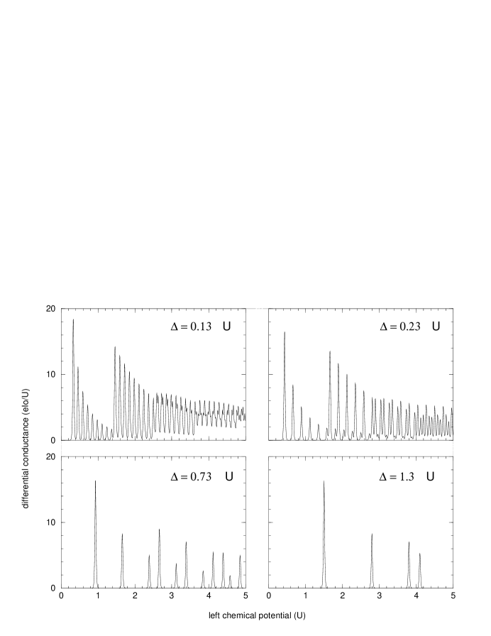
FIG. 3.: Differential conductance for various level spacings ($\Gamma_{L}=\Gamma_{R}$)

FIG. 4.: Ohmic conductance through a dot with discrete levels ($\Delta_{\epsilon}=0.1U$)

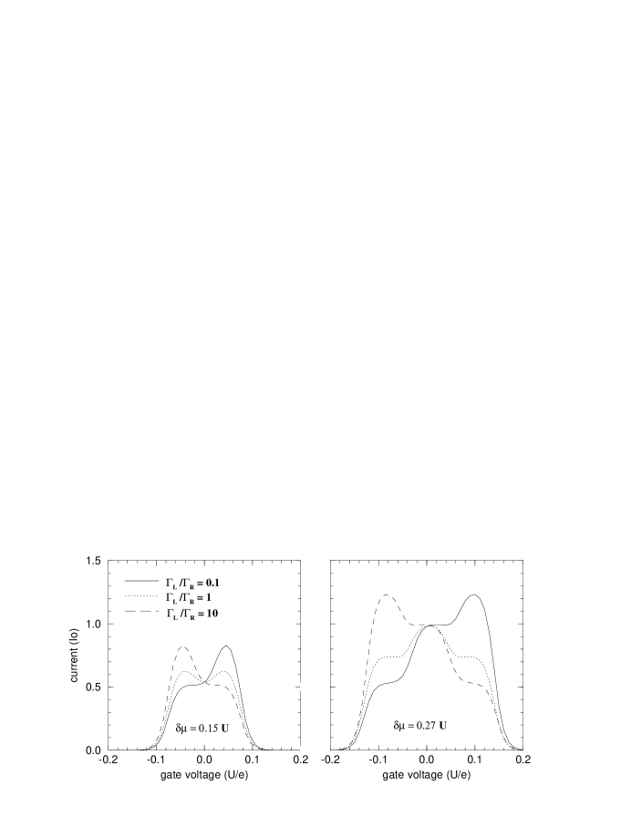
FIG. 5.: Current vs gate voltage at fixed bias ($\Delta_{\epsilon}=0.1U$)

FIG. 6.: Energy dependence of the inter-dot transition rate: (a) ignoring level broadening, (b) including broadening $\Gamma_{\phi}=5V_{M}$.

FIG. 7.: Ohmic conductance through a double dot with $A_{ph}\hbar/\Gamma=1$ ($U_{1}=0.41U$, $U_{2}=U$, $\Delta_{\epsilon_{1}}=0.13U$, $\Delta_{\epsilon_{2}}=0.32U$). The empty and filled circles indicate the positions at which the average occupation increases by one for dot $1$ and $2$ respectively.

FIG. 8.: Temperature at which a conductance peak reaches its maximum

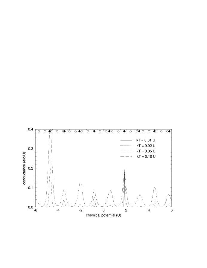
FIG. 9.: Ohmic conductance through a double dot with $A_{ph}\hbar/\Gamma=0.01$ ($U_{1}=0.41U$, $U_{2}=U$, $\Delta_{\epsilon_{1}}=0.13U$, $\Delta_{\epsilon_{2}}=0.32U$). The empty and filled circles indicate the positions at which the average occupation increases by one for dot $1$ and $2$ respectively.

FIG. 10.: I-V characteristics for a double dot at various temperatures ($U_{1}=0.41U$, $U_{2}=U$, $\Delta_{\epsilon_{1}}=0.13U$, $\Delta_{\epsilon_{2}}=0.32U$, $A_{ph}\hbar/\Gamma=0.01$)

FIG. 11.: I-V characteristics for a double dot at various temperatures (the dots are interchanged with respect to the previous figure)

FIG. 12.: Energy diagram for tunnelling through two dots at fixed bias

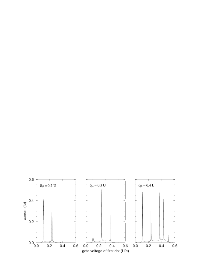
FIG. 13.: Current vs gate voltage of first dot at fixed bias ($U_{1}=0.41U$, $U_{2}=U$, $\Delta_{\epsilon_{1}}=0.13U$, $\Delta_{\epsilon_{2}}=0.32U$, $k_{B}T=0.02U$, $\Gamma_{L}=\Gamma_{R}=\Gamma$, $A_{\rm ph}\hbar/\Gamma=0.01$)

REFERENCES

- [1]
- [2] B.J. van Wees, H. van Houten, C.W.J. Beenakker, J.G. Williamson, L.P. Kouwenhoven, D. van der Marel, C.T. Foxon, Phys. Rev. Lett.60, 848 (1988).
- [3] D.A. Wharam, T.J. Thornton, R. Newbury, M. Pepper, H. Ahmed, J.E.F. Frost, D.G. Hasko, D.C. Peacock, D.A. Ritchie, G.A.C Jones, J. Phys. C 21, L209 (1988).
- [4] J.H.F. Scott-Thomas, S.B. Field, M.A. Kastner, H.I. Smith, D.A. Antoniadis, Phys. Rev. Lett.62, 583 (1989).
- [5] H. van Houten, C.W.J. Beenakker, Phys. Rev. Lett.63, 1893 (1989).
- [6] M.A. Reed, J.N. Randall, R.J. Aggarwal, R.J. Matyi, T.M. Moore, A.E. Wetsel, Phys. Rev. Lett.60, 535 (1988).
- [7] M. Amman, R. Wilkins, E. Ben-Jacob, P.D. Maker, R.C Jaklevic, Phys. Rev. B43, 1146 (1991).
- [8] I.M. Ruzin, V. Chandrasekhar, E.I. Levin, L.I. Glazman, Phys. Rev. B45, 13469 (1992).
- [9] M. Kemerink, L.W. Molenkamp, Appl. Phys. Lett. 65, 1012 (1994).
- [10] Y. Meir, N.S. Wingreen, P.A. Lee, Phys. Rev. Lett.66, 3048 (1991).
- [11] C.W.J. Beenakker, Phys. Rev. B44, 1646 (1991).
- [12] D.V. Averin, A.N. Korotkov, K.K. Likharev, Phys. Rev. B44, 6199 (1991).
- [13] D. Weinmann, W. Häusler, W. Pfaff, B. Kramer, U. Weiss, Europhysics Lett. 26, 467 (1994).
- [14] D. Weinmann, W. Häusler, B. Kramer, Phys. Rev. Lett.74, 984 (1995).
- [15] U. Meirav, M.A. Kastner, S.J. Wind, Phys. Rev. Lett.65, 771 (1991).
- [16] A.T. Johnson, L.P. Kouwenhoven, W. de Jong, N.C. van der Vaart, C.J.P.M. Harmans, C.T. Foxon, Phys. Rev. Lett.69, 1592 (1992).
- [17] E.B. Foxman, P.L. McEuen, U. Meirav, N.S. Wingreen, Y. Meir, P.A. Belk, N.R. Belk, M.A. Kastner, S.J. Wind, Phys. Rev. B47, 10020 (1993).
- [18] N.C. van der Vaart, A.T. Johnson, L.P. Kouwenhoven, D.J. Maas, W. de Jong, M.P. de Ruyter van Steveninck, A. van der Enden, C.J.P.M. Harmans, Physica B 189, 99 (1993).
- [19] N.S. Wingreen, K.W. Jacobsen, J.W. Wilkins, Phys. Rev. Lett.61,1396 (1988).
- [20] W. Cai, T.F. Zheng, P. Hu, B. Yudanin, M. Lax, Phys. Rev. Lett.63, 418 (1989).
- [21] L.P. Kouwenhoven, S. Jauhar, K. McCormick, D. Dixon, P.L. McEuen, Y.V. Nazarov, N.C. van der Vaart, C.T. Foxon, Phys. Rev. B50, 2019 (1994).
- [22] K. Hess, C.T. Sah, Phys. Rev. B10, 3375 (1974).
- [23] A.D. Stone, P.A. Lee, Phys. Rev. Lett.54, 1196 (1985).
- [24] A.A.M. Staring, H. van Houten, C.W.J. Beenakker, Phys. Rev. B45, 9222 (1992).
- [25] N.C. van der Vaart, S.F. Godijn, Y.V. Nazarov, C.J.P.M. Harmans, J.E. Mooij, Phys. Rev. Lett.74, 4702 (1995).