BOUND STATES AND THRESHOLD RESONANCES IN QUANTUM WIRES WITH CIRCULAR BENDS

Abstract

We study the solutions to the wave equation in a two-dimensional tube of unit width comprised of two straight regions connected by a region of constant curvature. We introduce a numerical method which permits high accuracy at high curvature. We determine the bound state energies as well as the transmission and reflection matrices, ${\cal T}$ and ${\cal R}$ and focus on the nature of the resonances which occur in the vicinity of channel thresholds. We explore the dependence of these solutions on the curvature of the tube and angle of the bend and discuss several limiting cases where our numerical results confirm analytic predictions.

I Introduction

The problem of a quantum particle confined to a two-dimensional tube consisting of two straight regions connected by a region of arbitrary curvature but constant width, $d$, has aroused interest in recent years because of its applications in both the physics of small devices and electromagnetic waveguides.[1, 2, 4] Related geometries such as crossed wires[5] and elbows[3] have also been studied extensively. The primary focus has been on the existence of unanticipated bound states and on the “adiabatic” limit where the radius of curvature is always much greater than the width of the tube.[6] Goldstone and Jaffe proved that such a tube always has a bound state, with energy below the continuum threshold at $E={\hbar^{2}\over 2m}{\pi^{2}\over d^{2}}$.[7]

In this paper, we study the specific case where the curved region is an arc of a circle. This case can be solved numerically with relative ease, providing a laboratory in which to explore phenomena we believe to be quite general but difficult to demonstrate in arbitrary geometries. We take the tube to have unit width. We use the arc length, $s$, along the outer boundary of the tube as one coordinate, and the distance $y$, along the normal from the outer boundary toward the center of the circle as the other coordinate. We mark the boundaries of the curved region as $\pm s_{0}$. The angle subtended by the arc of the curved region is defined to be $\theta$, and it satisfies the relation $\theta=2\kappa s_{0}$, where $\kappa$ is the curvature (here a constant). Figure 1 shows two examples of such a tube. Notice that we allow ourselves to consider tubes with $\theta>\pi$ although such configurations require excursions from strictly planar geometry. Also, we choose units such that $\hbar^{2}/2m=1$ making $E=k^{2}$ dimensionless.

                                                                                              

FIG. 1.: An infinite two-dimensional tube of unit width comprised of two straight regions connected by a region of constant curvature $\kappa$. (a) $\theta<\pi$. (b) $\theta>2\pi$.

Scattering in a bent tube is a relatively simple example of a multichannel problem. Incoming and outgoing waves are labelled by an integer, $n$, the number of non-trivial nodes in the transverse wavefunction, $\sin n\pi y$. The scattering is described by transmission and reflection matrices ${\cal T}_{mn}$ and ${\cal R}_{mn}$ whose dimension grows as each successive channel threshold (at $E_{n}=n^{2}\pi^{2}$) is passed. In Ref. [7] it was pointed out that the same argument which demonstrates the existence of a bound state, also proves that there is a “quasibound” state just below each channel threshold. The quasibound state below the $N^{th}$ channel threshold would be stable and normalizable if all lower channels ($n<N$) were artifically closed. Such quasibound states should appear as resonances in the open channel scattering amplitudes.

Our aim in considering this solvable special case is to explore the systematics of the bound states as they depend on $\kappa$ and $\theta$, and to elucidate the character of the channel threshold resonances. Other workers have studied quantum wires with circular bends. Lent studied scattering in tubes with $\theta=\pi/2$ and showed that even for the largest curvature tractible there is very little reflection except at values of the energy just above the threshold.[8] Sols and Macucci have confirmed this result and discovered the presence of resonances associated with quasi-bound states just below propagation thresholds.[9] Moreover, they found that at large angles, more than one bound state may develop, and that the binding energy of these bound states increases as the curvature or angle is increased.

In §II, we establish a formalism for solving for both bound and scattering states in tubes with circular bends. We begin traditionally – by representing the solution in the curved region in terms of Bessel functions and imposing the standard continuity conditions at $s=\pm s_{0}$. Normally one would match the open channels to incoming and outgoing waves and the closed channels to falling exponentials. The matching conditions generate a linear algebra problem, which leads eventually to an eigenvalue problem (for the bound states) and a solution for ${\cal T}_{mn}$ and ${\cal R}_{mn}$ (for the scattering problem). However, we find that this approach leads to serious convergence problems at high curvature. At this point we abandon the traditional approach and formuate a novel method (as far as we are aware) where we match the interior wavefunction to both rising and falling exponentials in closed channels. We then seek solutions by minimizing the coefficients of the rising exponentials. We argue that this approach should converge more rapidly and reliably. We believe this method has wider application than the problem at hand. Also in this section we derive a small $\kappa$ approximation to the transmission amplitude in regions far from thresholds and resonances.

In §III we study the convergence of our method of calculating both scattering and bound states. We show that it is more convergent and more efficient than the traditional method (of allowing only falling exponentials in closed channels).

In §IV, we present results for the bound state eigenenergies and the scattering coefficients as functions of curvature and angle. We show that at fixed curvature, further bound states appear with increasing $\theta$. As $\theta\rightarrow\infty$, so does the number of bound states. The binding energy of the ground state approaches a limit determined by the root of a simple Bessel equation as $\theta\rightarrow\infty$. For $\kappa=1$ the limit is the square of the first zero of $J_{0}$ ($\approx(2.405)^{2}$). The higher bound state energies approach the same limit as the ground state, but more slowly. We also find the angle at which the first excited state appears, as a function of $\kappa$, and give a theoretical explanation why this angle approaches $2\pi$ as $\kappa$ approaches zero. We also plot the scattering coefficients ${\cal T}$ and ${\cal R}$ as functions of the energy and verify the presence of resonances associated with quasi-bound states just below the propagation threshold for each channel. Finally, we explore the behavior of ${\cal R}$ and ${\cal T}$ in the complex plane. We explain why the elastic transmission amplitude ${\cal T}_{11}$ drops to zero at the energy of the quasibound state just below the second threshold, $E=4\pi^{2}$, an effect which is echoed in other components of ${\cal T}$ at higher thresholds. At the same time we verify the predictions of the small $\kappa$ approximation for low curvature.

II Theory

In this section we summarize the basic formalism common to both the bound and scattering state problems. We then specialize to the bound state case and finally, to the scattering case.

A General Formalism

We are interested in the solutions to the wave equation, $-\vec{\nabla}^{2}\psi=k^{2}\psi$ within a “tube” coordinatized by $s$ and $y$. $\psi$ vanishes on the boundaries, $y=0$ and $1$, and we require that $\psi$ and and its normal derivative be continuous at $s=\pm s_{0}$ where the curvature of the tube jumps abruptly from zero to $\kappa$. We treat the curved and straight regions at the same time, taking $\kappa=0$ for the straight region. The coordinate differential is given by $d\vec{x}=\hat{s}ds(1-\kappa y)+\hat{y}dy$, and the differential area element is $d^{2}x=dsdy(1-\kappa y)$. Thus, the wave equation becomes

$$\kappa\frac{\partial}{\partial y}\psi-(1-\kappa y)\frac{\partial^{2}}{\partial y^{2}}\psi-\frac{1}{1-\kappa y}\frac{\partial^{2}}{\partial s^{2}}\psi=(1-\kappa y)k^{2}\psi.$$ (1)

We now make the standard change of variable, $\psi=\frac{1}{\sqrt{1-\kappa y}}\phi$ so that eq. (1) becomes

$$-\frac{\partial^{2}\phi}{\partial y^{2}}-\left[\frac{1}{(1-\kappa y)^{2}}\frac{\partial^{2}}{\partial s^{2}}+\frac{\kappa^{2}}{4(1-\kappa y)^{2}}\right]\phi=k^{2}\phi,$$ (2)

If we define $r\equiv 1-\kappa y$, and separate variables we recognize the radial equation as Bessel’s equation, with solutions of the form,

$$\psi_{l}(s,r)=\frac{1}{\sqrt{r}}S_{l}(s){\cal Y}_{l}(r),$$ (3)

where

$${\cal Y}_{l}(r)=\sqrt{r}\left[Y_{\nu_{l}}\left(\frac{kr}{\kappa}\right)J_{\nu_{l}}\left(\frac{k}{\kappa}(1-\kappa)\right)-J_{\nu_{l}}\left(\frac{kr}{\kappa}\right)Y_{\nu_{l}}\left(\frac{k}{\kappa}(1-\kappa)\right)\right]$$ (4)

and

$$S_{l}(s)=\left\{\begin{array}[]{l}\cos\kappa\nu_{l}s\\ \sin\kappa\nu_{l}s\end{array}\right..$$ (5)

Here $J_{\nu}$ and $Y_{\nu}$ are Bessel and Neumann functions respectively. The linear combination of Bessel functions in eq. (4) satisfies ${\cal Y}=0$ at $y=1\,(r=1-\kappa)$. The order, $\nu_{l}$, must be chosen to satisfy ${\cal Y}=0$ at $y=0\,(r=1)$. $\nu_{l}$ may be either real or imaginary, as we discuss below. The label $l=1,2,\ldots$ denotes the number of non-trivial nodes ($l-1$) in ${\cal Y}(r)$.

To study the character of $\nu_{l}$, we substitute eqs. (4) and (5) back into the wave equation. We find that the momentum satisfies the relation,

$$k^{2}=\kappa^{2}\nu_{l}^{2}+\xi_{l},$$ (6)

where $\xi_{l}$ is a positive term that grows with $l$. Thus, for fixed $k^{2}$ only a finite number of eigenvalues, $\nu_{l}^{2}$, can be positive. For any $k^{2}$ greater than $\pi^{2}$ there is at least one positive $\nu^{2}$ – a fact which is closely related to the existence of a bound state. As $k$ increases, more positive $\nu^{2}$ values appear – associated with the channel threshold resonances discussed below. Let $l\leq\ell$ correspond to real $\nu$ and $l>\ell$ give imaginary $\nu$, where we define $\beta\equiv i\nu$. Then,

$$\psi_{<}(s,r)=\frac{1}{\sqrt{r}}\sum_{l=1}^{\ell}a_{l}{\cal Y}_{l}(r)\left\{\begin{array}[]{l}\cos\kappa\nu_{l}s\\ \sin\kappa\nu_{l}s\end{array}\right\}+\frac{1}{\sqrt{r}}\sum_{l=\ell+1}^{\infty}a_{l}{\cal Y}_{l}(r)\left\{\begin{array}[]{l}\cosh\kappa\beta_{l}s\\ \sinh\kappa\beta_{l}s\end{array}\right\}.$$ (7)

We have added the subscript “$<$” to $\psi$ to denote the solution inside the circular region.

Depending on $k^{2}$, the exterior solutions, $|s|>s_{0}$, either oscillate or vary exponentially with $s$. The general exterior solution is of the form,

$$\psi_{>}=\sum_{m=1}^{\infty}(b_{m}e^{-\gamma_{m}(s-s_{0})}+c_{m}e^{\gamma_{m}(s-s_{0})})\sin m\pi y.$$ (8)

where

$$\gamma_{m}=\sqrt{m^{2}\pi^{2}-k^{2}}.$$ (9)

When $k^{2}>m^{2}\pi^{2},\,\gamma_{m}$ becomes imaginary and the solutions become oscillatory. In that case we define $\gamma_{m}\equiv ik_{m}$ with $k_{m}>0$.

We now apply continuity conditions at $s=s_{0}$, recalling that in the interior region the normal derivative of $\psi_{<}$ is

$$\hat{s}\cdot\vec{\nabla}\psi_{<}=\frac{1}{r}\frac{\partial}{\partial s}\psi_{<},$$ (10)

and we find

$$b_{m}+c_{m} = 2\sum_{l=1}a_{l}S_{l}(s_{0})M_{ml}$$ (11)

$$-b_{m}+c_{m} = \frac{2}{\gamma_{m}}\sum_{l=1}a_{l}\frac{dS_{l}}{ds}\left.\right|_{s=s_{0}}N_{ml}$$ (12)

where $M_{ml}=\int_{0}^{1}dy\sin m\pi y\frac{{\cal Y}_{l}}{\sqrt{r}}$ and $N_{ml}=\int_{0}^{1}dy\sin m\pi y\frac{{\cal Y}_{l}}{r^{3/2}}$. Eqs. (12) give an infinite dimensional matrix linear algebra problem to solve for the energies of bound states or the ${{\cal S}}$–matrix for scattering states. In practice we must truncate the sum over internal and external channels. We superpose $L$ internal solutions and attempt to match to $M$ external channels.

When $k^{2}<N^{2}\pi^{2}$ the $\{c_{m}\}$ with $m>N$ are coefficients of exponentially rising solutions. Because these solutions are not normalizable, standard practice is to dismiss them as unphysical and set $\{c_{m}\}$ for $m>N$ to zero from the beginning. This leads to an eigenvalue condition for $k$ which has unique solutions only when $L=M$, i.e. one is forced to use channel spaces of the same dimension both inside and outside the region of curvature. As the dimension of this channel space $(L=M)$ is increased, the accuracy of the solution should improve. After all, it corresponds to taking more terms in the approximation to the wavefunction. However, we have found that this straightforward approach fails at high curvature ($\kappa>0.6$). As the channel space dimension is increased, the solution does not seem to converge. We believe that this is due to poor matching at the boundary $s=s_{0}$: We expect that an interior function with $n$ nodes should match to a superposition of exterior functions dominated by terms with $n$, $n\pm 1$, and $n\pm 2$, etc. nodes. However, the $L=M$ restriction forbids the introduction of any exterior functions with higher frequencies than the interior functions, so that the $n+1$, $n+2$ node terms are not present. Clearly it would be advantageous to allow $M>L$. However, a simple count of the number of degrees of freedom shows that the there is no solution under these circumstances.

To solve this problem, we have implemented a novel approach: we retain the rising exponentials and seek first the set of $\{a_{l}\}$ and next the value of $k$ for which $\sum_{m=1}^{M}c_{m}^{2}$ is minimized. As we shall see, this approach removes the $L=M$ restriction, allowing us to take as many terms in either sum as we like. Of course, in the limit $L,M\rightarrow\infty$, $\{c_{m}\}\rightarrow 0$ in the closed channels for all physically interesting solutions, whether bound or scattering.

B Bound state formalism

Bound states correspond to solutions of Eqs. (12) with $k^{2}<\pi^{2}$. Our strategy will be to allow the $\{c_{m}\}$ to be non-zero and seek solutions which minimize $\sum_{m=1}^{M}c_{m}^{2}$. We anticipate that the parity of the ground state will be even, so we choose internal solutions which are superpositions of $\cos\kappa\nu s$ or $\cosh\kappa\beta s$. If there are several bound states, this symmetric ansatz will find the even ones. A corresponding ansatz odd under $s\leftrightarrow-s$ finds the odd states. Even and odd bound states alternate as a function of the energy.

We use the method of Lagrange multipliers to minimize $\sum c_{m}^{2}$ subject to the constraint that $\sum_{l=1}^{L}a_{l}^{2}=1$. There is some arbitrariness in this prescription. The $\{a_{l}\}$ must be constrained in some way, otherwise the trivial solution $\{a_{l}\}=0$ will follow. The sensitivity of our method to the form of the constraint is discussed in the following section. We define

$$\Delta(\{a_{l}\},k)\equiv\sum_{m=1}^{M}c_{m}^{2}(\{a_{l}\})-\lambda(\sum_{l=1}^{L}a_{l}^{2}-1)$$ (13)

and seek to minimize $\Delta$ first with respect to the $\{a_{l}\}$ and then with respect to k. The conditions $\frac{\partial\Delta}{\partial a_{l}}=0$, lead to an algebraic problem, with a solution $\{a_{l}^{0}(k)\}$. Substituting back into eq. (13), $\Delta$ reduces to a function of $k$, whose minima we locate numerically.

First we combine eqs. (12) to obtain $c_{m}$ as a function of the $\{a_{l}\}$,

$$c_{m} = \sum_{l=1}^{L}{\cal G}_{ml}a_{l},\quad{\rm where}$$ (14)

$${\cal G}_{ml} = M_{ml}S_{l}(s_{0})+\frac{1}{\gamma_{m}}N_{ml}S^{\prime}_{l}(s_{0}).$$ (15)

Next we substitute for $c_{m}$ in eq. (13), and differentiate with respect to $a_{l}$ to obtain,

$$\sum_{j=1}^{L}\Xi_{lj}a_{j} = \lambda a_{l},\quad{\rm where}$$ (16)

$$\Xi_{lj} = \sum_{m=1}^{M}{\cal G}_{ml}{\cal G}_{mj}$$ (17)

This is an $L$ dimensional, matrix eigenvalue problem. The external channel space dimension, $M$, appears in the definition of $\Xi$, but does not complicate eq. (17). Since $\Xi$ is a positive definite matrix, it has real, positive eigenvalues, $\lambda^{1}(k)$, $\lambda^{2}(k)$ etc., ordered from smallest to largest, and associated eigenvectors, $a_{l}^{1}$, $a_{l}^{2}$, etc. Each eigenvector gives a stationary point of the functional $\Delta$. Normalizing $\sum_{l=1}^{L}(a^{i}_{l})^{2}=1$ as required by the constraint it is easy to see that

$$\Delta(\{a_{l}^{i}(k)\},k)=\sum_{m=1}^{M}c_{m}^{2}(\{a_{l}^{i}\})=\lambda^{i}(k),$$ (18)

so the smallest eigenvalue gives the minimum $\Delta(k)$ at fixed $k$. To find the best approximation to the bound states for fixed $L$ and $M$, we search for a value of $k<\pi$ that minimizes the lowest eigenvalue, $\lambda^{1}(k)$. The magnitude of $\lambda^{1}(k)$ measures the squared sum of coefficients of rising exponentials, and is a measure of the accuracy of our solution. There is always at least one minimum of $\lambda^{1}(k)$ for $k<\pi$ — a consequence of the general theorem of Ref. [7]. For small values of $s_{0}$, there is only one minimum at $k\equiv\bar{k}_{1}$, corresponding to a ground state energy of $\bar{k}_{1}^{2}$. As $s_{0}$ is increased (at fixed $\kappa$), there will be multiple minima of $\lambda^{1}(k)$ which we denote by $\bar{k_{1}}$, $\bar{k_{3}}$, $\bar{k_{5}}$, etc., with $\bar{k_{p}}<\pi$. ($\bar{k_{1}}$ corresponds to the ground state, $\bar{k_{3}}$ to the second excited state, and so on.) The odd-numbered excited states ($p$ even) are antisymmetric in $s$ and are obtained from an antisymmetric ansatz.

We must set the number of terms in the sums in eqs. (17) to values such that the computations are tractable while still retaining reasonable accuracy. Studies of convergence and accuracy are presented in §III. We emphasize, though, that the convergence is not a trivial issue for this problem: the default assumption, $L=M$, fails to converge as $L\rightarrow\infty$ for interesting values of $\kappa$, forcing us to take a different approach. Anticipating the results of §III, we note that the results presented in §IV were obtained with $L=4$ and $M=10$, which generated accuracy to about five decimal places.

C Formalism for scattering states

We now extend our formalism to handle scattering solutions. At an energy $E=k^{2}$, the “longitudinal” momentum in the $n^{th}$ channel is $k_{n}=\sqrt{k^{2}-n^{2}\pi^{2}}$. If $N^{2}\pi^{2}<k^{2}<(N+1)^{2}\pi^{2}$, then $N$ channels are “open”: for $n\leq N$, $k_{n}$ is real and wavefunctions in the external regions are oscillatory. For $n>N$, $k_{n}$ is imaginary. These channels are “closed”: we define $ik_{n}=\gamma_{n}$; the solutions are exponential as in the bound state problem. Since internal and external channel sums cover different ranges we will use different indices as follows: $i$, $j$, $k$, and $l$ label internal (curved region) solutions; and $m$, $n$, $p$, $q$, and $r$ label external (straight region) channels. $N$ will always denote the number of open channels.

An incident wave in the $q^{th}$ channel will couple to all channels. However, the solutions in the closed channels die exponentially, so that at a distance (s $\rightarrow\pm\infty$), we see reflection and transmission in only the open channels. We wish to solve for these ${\cal R}$ and ${\cal T}$ coefficients and explore their behavior as functions of the channel and energy of the incoming wave as well as the parameters of the tube. Unlike the bound state problem, this is not an eigenvalue problem. There are many solutions (in fact $2N$) for each value of the energy. Our aim is to find the solutions and parametrize them in terms of the matrices ${\cal R}$ and ${\cal T}$.

Since our internal solutions are naturally constructed as either symmetric or antisymmetric (in $s$), it is convenient to do likewise with the external solutions. We consider the symmetric case explicitly — from which we will obtain ${\cal T}+{\cal R}$. The antisymmetric case proceeds along identical lines and yields ${\cal T}-{\cal R}$. The solutions are labelled by the indices $q$, the channel of the incoming wave, and $p$, the channel under consideration. The symmetric solution is the sum of the left- and right-incoming solutions:

$$s\rightarrow\pm\infty:\sigma^{q}_{p}(s)=\frac{1}{\sqrt{ik_{p}}}(\delta_{pq}e^{-ik_{p}|s|}+({\cal T}+{\cal R})_{pq}e^{+ik_{p}|s|})$$ (19)

Unitarity requires $({\cal T}+{\cal R})^{\dagger}({\cal T}+{\cal R})=1$, and from the antisymmetric solution, $({\cal T}-{\cal R})^{\dagger}({\cal T}-{\cal R})=1$, or

$${\cal T}^{\dagger}{\cal T}={\cal R}^{\dagger}{\cal R} =1,$$ (20)

$${\cal T}^{\dagger}{\cal R}+{\cal R}^{\dagger}{\cal T} =0.$$ (21)

These constraints can be summarized by the requirement that the matrix

$${\cal S}=\left(\begin{array}[]{cc}{\cal R}&{\cal T}\\ {\cal T}&{\cal R}\end{array}\right)$$ (23)

be unitary, ${\cal S}^{\dagger}{\cal S}=1.$ This is a special case (for Hamiltonians symmetric under $s\rightarrow-s$) of the general definition of the ${\cal S}$–matrix,

$${\cal S}=\left(\begin{array}[]{cc}{\cal R}&{\cal T}^{\prime}\\ {\cal T}&{\cal R}^{\prime}\end{array}\right)$$ (24)

where ${\cal R}$ and ${\cal T}$ are reflection and transmission coefficients for waves incident from the left and ${\cal R}^{\prime}$ and ${\cal T}^{\prime}$ are the analogous coefficients for right incident waves. Time reversal invariance requires ${\cal S}^{T}={\cal S}$, which requires ${\cal T}^{T}={\cal T}$ and ${\cal R}^{T}={\cal R}$ for symmetric Hamiltonians.[10]

To solve for the matrices ${\cal T}$ and ${\cal R}$, we return to the basis wavefunctions for the bound state problem, modified to accommodate the open channels and the factor of $\sqrt{ik}$. Note that this factor is present only in the open channels where $n\leq N$. Because our solution is symmetric, we take $S_{l}(s)$ to be $\cos{\kappa\nu_{l}s}$,

$$\psi^{q}_{<}(s,y) = \frac{1}{\sqrt{r}}\sum_{l}a_{l}^{q}Y_{l}(r)S_{l}(s)$$ (25)

$$\psi^{q}_{>}(s,y) = \sum_{n=1}^{N}\frac{1}{\sqrt{ik_{n}}}(b^{q}_{n}e^{-ik_{n}(s-s_{0})}+c^{q}_{n}e^{ik_{n}(s-s_{0})})\sin{n\pi y}$$ (26)

$$+ \sum_{n=N+1}^{M}(b^{q}_{n}e^{-\gamma_{n}(s-s_{0})}+c^{q}_{n}e^{\gamma_{n}(s-s_{0})})\sin{n\pi y}.$$ (27)

By comparing Eqs. (19) and (27) we can identify ${\cal T}+{\cal R}$ in terms of $b$ and $c$ for open channels,

$$b_{p}^{q} = \delta_{pq}e^{-ik_{p}s_{0}}$$ (28)

$$c_{p}^{q} = ({\cal T}+{\cal R})_{pq}e^{ik_{p}s_{0}}$$ (29)

for $p,q\leq N$. By analysis similar to the bound state problem, continuity at $s=s_{0}$ shows that

$$c^{q}_{n}=\sum_{l=1}^{L}{\cal G}_{nl}a_{l}^{q}$$ (30)

and

$$b^{q}_{n}=\sum_{l=1}^{L}{\cal H}_{nl}a_{l}^{q}$$ (31)

where

$${\cal G}_{nl}=\left\{\begin{array}[]{ll}\sqrt{ik_{n}}S_{l}(s_{0})M_{nl}+\frac{1}{\sqrt{ik_{n}}}S_{l}^{\prime}(s_{0})N_{nl}&n\leq N\\ S_{l}(s_{0})M_{nl}+\frac{1}{\gamma_{n}}S_{l}^{\prime}(s_{0})N_{nl}&n>N\end{array}\right.$$ (32)

and

$${\cal H}_{nl}=\left\{\begin{array}[]{ll}\sqrt{ik_{n}}S_{l}(s_{0})M_{nl}-\frac{1}{\sqrt{ik_{n}}}S_{l}^{\prime}(s_{0})N_{nl}&n\leq N\\ S_{l}(s_{0})M_{nl}-\frac{1}{\gamma_{n}}S_{l}^{\prime}(s_{0})N_{nl}&n>N\end{array}\right.$$ (33)

As in the bound state case, tradition would dictate setting the coefficients of growing exponentials in closed channels to zero ab initio. We seek to improve convergence and accuracy by instead keeping the growing exponentials and minimizing their contributions. We have found that the best convergence for high $\kappa$ is obtained by minimizing the ratio of the growing contributions relative to the falling contributions, i.e. minimizing $\sum_{n>N}|c_{n}|^{2}$ subject to the constraint that $\sum_{n>N}|b_{n}|^{2}=1$.

Because scattering boundary conditions are complex (viz. eq. (29)), we must be more careful about the reality properties of the variables we consider. Certainly $c_{n}$ and $b_{n}$ are complex in open channels. Likewise, the matrices ${\cal H}$ and ${\cal G}$ are complex, although they are clearly real for $n>N$. Our manipulations will be simplified considerably by using matrix notation. Even though ${\cal G}$ and ${\cal H}$ are not square matrices, there should be no ambiguity in the definition of quantities such as ${\cal G}^{\dagger}{\cal H}$, etc.. We define a matrix projection onto the closed channels: ${\cal P}_{mn}=0$, except ${\cal P}_{mm}=1$ when $M\geq m>N$. Note that ${\cal P}$ is an $M$ dimensional matrix in the external channel space.

For an incoming wave in the $q^{th}$ channel (suppressing the $q$ superscript), we can once again define the projection onto rising exponentials, and implement the constraint $\sum_{n>N}|b_{n}|^{2}=1$ by a lagrange multiplier,

$$\Delta({\vec{a}},k)\equiv\vec{a}^{\dagger}\Xi\vec{a}-\lambda(\vec{a}^{\dagger}\Omega\vec{a}-1)$$ (34)

where $\Xi\equiv{\cal G}^{\dagger}{\cal P}{\cal G}$ and $\Omega\equiv{\cal H}^{\dagger}{\cal P}{\cal H}$. Note that $\Xi$ and $\Omega$ are both real, symmetric matrices in the internal ($L$–dimensional) space. In practical calculations, $L$ is small (compared to the external channel space dimension, $M$), so these matrices are relatively easy to manipulate.

It is convenient to work in the basis of eigenvectors of $\Omega$. Let $\{\vec{v}^{k},k=1,L\}$ be the orthonormal eigenvectors of $\Omega$ corresponding to (real, positive) eigenvalues $\{\omega_{k}\}$,

$$\Omega\vec{v}^{k} = \omega_{k}\vec{v}^{k}$$ (35)

$$\vec{v}^{k\dagger}\cdot\vec{v}^{l} = \delta_{kl}.$$ (36)

We rewrite $\vec{a}$ in the basis of the $\{\vec{v}^{k}\}$, using $\sqrt{\omega_{k}}$ as a metric,

$$\vec{a}=\sum_{k=1}^{L}\frac{1}{\sqrt{\omega_{k}}}\eta_{k}\vec{v}^{k}.$$ (37)

Inserting this definition back into eq. (34), we obtain

$$\Delta(\{\vec{\eta}\},k)=\vec{\eta}^{\,\dagger}\,\widetilde{\Xi}\,\vec{\eta}-\lambda(\vec{\eta}^{\,\dagger}\,\vec{\eta}-1).$$ (38)

where

$$\widetilde{\Xi}^{kl}={1\over\sqrt{\omega_{k}\omega_{l}}}\vec{v}^{k\dagger}\,\Xi\,\vec{v}^{l}$$ (39)

Now, the condition $\frac{\partial\Delta}{\partial\vec{a}^{\dagger}}=0$ becomes

$$\frac{\partial\Delta}{\partial\vec{\eta}^{\,\dagger}}=0\Longrightarrow\widetilde{\Xi}\,\vec{\eta}=\lambda\,\vec{\eta},$$ (40)

an $L$ dimensional eigenvalue problem with solutions $\{\vec{\eta}^{q}\,{\rm and}\,\lambda^{q},\,{\rm for}\,q=1,L\}$. As in the bound state case, the eigenvalue $\lambda^{q}$ is the value of $\Delta$ at the stationary point. Small $\lambda^{q}$ therefore correspond to solutions to the wave equation with negligible projection on exponentially growing solutions in the closed channels and are therefore physically interesting.

The number of physically significant solutions to this eigenvalue problem depends on the energy, $k^{2}$. Below the lowest threshold, $k^{2}<\pi^{2}$, we do not expect (and did not find) any solutions with small $\Delta$ except at the energies of bound states. When one channel is open ($\pi^{2}\leq k^{2}<4\pi^{2}$), there should be a single symmetric solution to the wave equation for each energy. So we expect to find one eigenvalue, $\lambda^{1}$, much smaller than the rest. When a second channel opens, there are now two symmetric solutions, so we expect to find two small eigenvalues, $\lambda^{1}$ and $\lambda^{2}$. We conclude that we must expand the vector $\vec{a}$ as a linear combination of the $N$ eigenvectors associated with the lowest $N$ eigenvalues when $N$ channels are open. We now expand the vector $\vec{a}$ in terms of the lowest $N$ eigenvectors $\vec{\eta}^{r}$ of $\widetilde{\Xi}$:

$$\vec{a}=\sum_{r=1}^{N}d_{r}\sum_{k=1}^{L}\frac{1}{\sqrt{\omega_{k}}}\eta_{k}^{r}\vec{v}^{k},$$ (41)

where $d_{r}$ is the expansion coefficient and the sum over $k$ corresponds to the expansion in terms of $\eta^{k}$ as defined in eq. (37). Finally, we define the $L\times N$ matrix

$${\cal M}_{jr}=\sum_{k=1}^{L}\frac{1}{\sqrt{\omega_{k}}}\eta_{k}^{r}v^{k}_{j}$$ (42)

so that we may write compactly

$$\vec{a}={\cal M}\vec{d}.$$ (43)

We are now prepared to return to our identifications of $b_{n}^{q}$ and $c_{n}^{q}$ from eq. (29). Inserting our above expression for $a_{i}$ into eq. (31), we find that

$$d_{n}^{q}={\cal Q}_{nq}^{-1}e^{ik_{q}s_{0}}$$ (44)

where ${\cal Q}$ is an $N\times N$ matrix defined by

$${\cal Q}={\cal H}{\cal M}.$$ (45)

Substituting eqs. (43) and (44) back into eq. (30) and recalling our identification with $({\cal T}+{\cal R})$ in eq. (29), we obtain at last

$$({\cal T}+{\cal R})_{pq}=\{G{\cal M}Q^{-1}\}_{pq}e^{i(k_{p}+k_{q})s_{0}}.$$ (46)

Note that in the end the matrix manipulations which are calculationally intensive — finding eigenvalues, eigenvectors and inverses — are only carried out on matrices of dimension $L$. The external channel index, $M$, can therefore be taken very much greater than $L$ without increasing the computation time significantly.

The antisymmetric scattering states can be analyzed in the same fashion, beginning with the parameterization of the scattering states,

$$s\rightarrow\pm\infty:\alpha^{q}_{p}(s)=\frac{1}{\sqrt{ik_{p}}}(\delta_{pq}e^{-ik_{p}|s|}+({\cal T}-{\cal R})_{pq}e^{+ik_{p}|s|})$$ (47)

obtained by subtracting the left- and right-incoming wave solutions. This allows us to solve for the quantity $({\cal T}-{\cal R})_{pq}$, which we then combine with eq. (46) to yield the desired matrices ${\cal T}$ and ${\cal R}$.

D Small curvature approximation for the transmission amplitude

When the curvature, $\kappa$, is small, the solutions to our problem simplify somewhat. There is a quite well developed theory of the adiabatic approximation for a quantum wire with small and slowly varying curvature — $\kappa\ll 1$ and ${d\kappa\over ds}\ll 1$ — but it does not apply to a circular region joining two straight regions because $\kappa$ jumps abruptly to zero at $s_{0}$. Also, most of the results are restricted to $sqrt(k^{2}-\pi^{2})\approx 0$. Nevertheless we can use the fact that $\kappa$ is small to simplify the calculation of the elastic scattering amplitudes ${\cal T}_{mm}$ and ${\cal R}_{mm}$ in regions away from resonances and bound states. The result is

$${\cal T}_{mm} = \left[1+{\cal O}(\kappa^{2})\right]\exp\left(-ik_{m}\theta\over 2+{\cal O}(k_{m}\kappa\theta)\right)$$ (48)

$${\cal R}_{mm} = {i\kappa\over 2}\sin(2k_{m}s_{0}-k_{m}\theta/2)\left[1+{\cal O}(\kappa)\right]\exp\left(-ik_{m}\theta\over 2+{\cal O}(k_{m}\kappa\theta)\right),$$ (49)

where $k_{m}=\sqrt{k^{2}-\pi^{2}}$ and these expressions are only valid when $k_{m}^{2}\gg\kappa^{2}$.

The derivation of these results begins from eq. (2), which we expand in a Fourier series, $\phi(s,y)=\sum_{n}f_{n}(s)\sin n\pi y$,

$$D_{mn}(f_{n}^{\prime\prime}+{\kappa^{2}\over 4}f_{n})+k_{m}^{2}f_{m}=0,$$ (50)

where

$$D_{mn}=2\int_{0}^{1}dy{\sin m\pi y\sin n\pi y\over(1-\kappa y)^{2}}.$$ (51)

Since $D_{mn}$ is of order $\kappa$ when $m\neq n$, it is easy to see that the effect of the $n^{th}$ channel on a wave incident in the $m^{th}$ channel begins at order $\kappa^{2}$. This confirms our decision to work only to order $\kappa$. To this order $D_{mm}=1+\kappa$, which makes this system unusual, since the perturbation appears in lowest order only in the kinetic term. In the end this will lead to the result that an arbitrarily small curvature can result in a large scattering phase provided the product $\kappa s_{0}\propto\theta$ is large.

Working to order $\kappa$ we can ignore the “potential” $\kappa^{2}/4$, with the result that $f_{m}\propto\exp\pm(iq_{m}s)$, where $q_{m}^{2}=k_{m}^{2}(1-\kappa+{\cal O}(\kappa^{2}))$. We now construct symmetric and antisymmetric combinations of these interior solutions, and match them and their normal derivatives to the appropriate external scattering states eqs. (19) and (47). Since channel coupling is of higher order in $\kappa$, ${\cal T}_{mm}\pm{\cal R}_{mm}$ are both unitary, so we parametrize them by phases, ${\cal T}_{mm}\pm{\cal R}_{mm}=\exp(2i\delta^{m}_{\pm})$. The result of the matching calculation is

$$\tan(k_{m}s_{0}+\delta^{m}_{\pm})=(1\pm{\kappa\over 2}+{\cal O}(\kappa^{2}))\tan q_{m}s_{0}.$$ (52)

Note that $q_{m}s_{0}$ and $k_{m}s_{0}$ differ by $-k_{m}\kappa s_{0}/2$ which need not be small even when $\kappa\rightarrow 0$ because $2\kappa s_{0}=\theta$ can be held fixed in this limit. So the leading effect on ${\cal T}_{mm}$ and ${\cal R}_{mm}$ arises from this accumulating phase along the bending section. The prefactor $(1\pm{\kappa\over 2})$ determines the modulus of ${\cal T}_{mm}$ and $R_{mm}$. When we solve for $|{\cal T}_{mm}|$, we find that effects of order $\kappa$ cancel, which they must do since $|{\cal R}_{mm}|\sim\kappa$ and $|{\cal T}_{mm}|^{2}+|{\cal R}_{mm}|^{2}$ must give unity to order $\kappa^{2}$. This completes our derivation. The results, eqs. (49), give a useful approximation to the elastic amplitudes over much of their range when $\kappa\ll 1$.

III Computation and Convergence

The straightforward approach to solving the wave equation by matching interior to exterior solutions failed for physically interesting values of curvature and angle, forcing us to develop a different method of calculation. We are not aware of any studies of this method in the literature, and therefore present some details of our studies of convergence here. Readers not interested in calculational methods should skip directly to the results presented in §IV.

A Convergence of calculations for the bound state energies

The traditional method of matching $L$ independent internal solutions to $L$ independent external solutions does not converge as $L$ increases at large values of $\kappa$. This is illustrated graphically in Figure 2, where we plot the calculated ground state energy $\bar{k_{1}}$ as a function of $L$ for $\kappa=0.8$ and $\theta=\pi$. We have attributed this failure to converge to the absence of small wavelength (in $y$) states on the outside, necessary to accurately expand the internal states. In order to demonstrate that this is indeed the case, we have studied the convergence as a function of $L$ and $M$. Table I shows the effect on the calculated ground state energy $\bar{k_{1}}$ of varying the channel spaces $L$ and $M$ in the case where $\kappa=0.8$ and $\theta=\pi$. The best accuracy for the least amount of computation time is obtained by setting $M>L$. We can see from the lower left corner of the table that setting $M\leq L$ does not produce favorable results, because as higher-frequency interior functions enter the picture, we require even more high-frequency exterior functions for a good match at the boundary $s=s_{0}$.

                                                                    

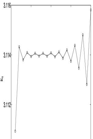
FIG. 2.: The eigenvalue $\bar{k_{1}}$ plotted as a function of the channel space in the case $L=M$, for $\kappa=0.8$,$\theta=\pi$. As the channel space is increased, the solution starts to converge but then begins to oscillate wildly.

$L$	$M$=5	$M$=10	$M$=30	$M$=50
1	2.9837e-03	2.9834e-03	2.9834e-03	2.9834e-03
2	5.5981e-05	5.4785e-05	5.4635e-05	5.4635e-05
3	8.3369e-05	7.2461e-05	7.2181e-05	7.2180e-05
4	6.0521e-06	9.3112e-06	9.1729e-06	9.1717e-06
5	7.4863e-05	1.0638e-05	9.9300e-06	9.9287e-06
6	2.6707e-03	1.6007e-06	2.2744e-06	2.2728e-06
7	7.6036e-03	4.1820e-06	2.3406e-06	2.3390e-06
8	8.3919e-04	3.6752e-06	5.7210e-07	5.7000e-07
9	4.7389e-03	9.8571e-06	5.7590e-07	5.7370e-07
10	9.7321e-04	6.9994e-05	2.9000e-09	0.0000e+00

TABLE I.: Tabulation of $|\bar{k_{1}}(L,M)-\bar{k_{1}}(10,50)|$ for $\kappa=0.8,\theta=\pi.$

We notice a few general trends in the convergence of $\bar{k_{1}}$. As expected, increasing $M$ at fixed $L$ improves the accuracy of the result. Note that the larger the value of $L$, the larger $M$ must be taken to capture this improvement. Note also that once the improvement has occured, there is little to be gained by further increasing $M$. So, for example, $L=5$ improves dramatically as $M$ increases from $5$ to $10$, and improves little thereafter. In contrast $L=9$ improves through $M=30$, and little thereafter. Also, for fixed $M$, the convergence worsens as $L$ is increased past the value of $M$, as we can see clearly in the $M=5$ case. Increasing the number of interior basis functions should improve the accuracy of the representation of the interior wavefunction, but apparently this is useless when the corresponding higher-frequency terms needed to match to the outside wavefunction are omitted, as is the case when $M\leq L$. As can be seen from the table, our parameters of $L=4$ and $M=10$ yield accuracy to about one part in $10^{6}$.

We also note that as the number of interior basis functions $L$ is increased, the value of $\Delta(\bar{k_{1}})=\sum c_{m}^{2}$ decreases, again provided that $M>L$. Table II illustrates this convergence for the same parameters $\kappa=0.8$ and $\theta=\pi.$ This is to be expected; as the bound state approximation is improved, the contributions of the exponentially rising terms should approach zero. Although the value of $\Delta(\bar{k_{1}})$ does not decrease for fixed L and increasing M, we suspect that this is a result of the increased number of terms in the sum $\sum_{m}^{M}c_{m}^{2}$, which offsets the expected decrease in rising exponential contributions.

For the case $L=M$, $\Delta(\bar{k_{1}})$ deviates from the trend in that it is many orders of magnitude smaller than for the other cases. This can be explained by recalling the traditional approach discussed in §II.A, where the coefficients of the rising exponential exterior functions are set to zero from the beginning. The resulting set of equations has solutions only when $L=M$. With our approach, we thus expect to find a solution where the sum of these coefficients $\Delta(\bar{k})$ is zero (limited only by machine precision) when $L=M$.

$L$	$M$=5	$M$=10	$M$=30	$M$=50
1	2.239313e-03	2.248376e-03	2.248825e-03	2.248828e-03
2	1.199955e-04	1.202554e-04	1.203799e-04	1.203814e-04
3	3.572416e-05	4.230296e-05	4.261721e-05	4.261908e-05
4	7.442269e-06	8.907401e-06	8.950761e-06	8.952150e-06
5	2.754173e-19	4.409149e-06	4.686405e-06	4.688083e-06
6	2.209942e-17	1.565973e-06	1.632015e-06	1.633293e-06
7	1.440247e-09	7.985669e-07	1.019960e-06	1.021530e-06
8	1.770510e-05	3.232110e-07	4.602362e-07	4.613563e-07
9	1.573734e-04	1.585803e-07	3.173988e-07	3.188958e-07
10	7.881601e-02	2.996393e-19	1.676304e-07	1.685153e-07

TABLE II.: $\Delta(\bar{k_{1}})$ for $\kappa=0.8,\theta=\pi$ with varying channel space $L$ and $M$.

B Convergence of different methods for scattering states

In our study of scattering we explored further the choice of constraint in the Lagrange multiplier problem. One obvious choice is simply to constrain our solution to match to the asymptotic conditions in a channel of interest, namely that the equations for $b_{n}^{q}$ (eq. (31)) must be satisfied in the open channels. Our equation for $\Delta$ would then require a Lagrange multiplier for each separate channel, leading to

$$\Delta=\sum_{m=N+1}^{M}(G_{ml}^{\ast}a_{l}^{\ast})(G_{mj}a_{j})-\sum_{n=1}^{N}\lambda_{n}(H_{nl}a_{l}-b_{n}).$$ (53)

We note that the incoming channel label, $q$, introduced in §II.C, which should appear on $\Delta,a_{j},$ and $b_{n}$, has been suppressed for clarity.

Extremizing this expression for $\Delta$ yields a set of equations from which we can determine $a_{l}$ and $\lambda_{n}$ in a straightforward manner. However, we have found that this method has poor convergence for large $\kappa$. Next we considered the same condition as used for the bound states, namely eq. (13) with the extension that the coefficients $a_{l}$ may now be complex. While this second method converges for significantly higher values of $\kappa$ than the previous method, we get even slightly better convergence with the procedure outlined in §II.C, in which we use the constraint $\sum|b_{n}^{q}|^{2}=1$.

Table III illustrates the convergence of $|{\cal R}_{11}|$ for different $L$ and $M$ in the case $k=6.28$, $\kappa=0.9$, and $\theta=\pi/2$ for the constraints $H_{nl}a_{l}=b_{n}$ and $\sum|b_{n}|^{2}=1$. This is a region — near the second threshold at $2\pi$ and at large $\kappa$ — where convergence is problematic. By examining $|{\cal R}_{11}(L,M)-{\cal R}_{11}(14,24)|$ for the two choices of constraint, we see that convergence is better for the second method. This is primarily due to the fact that for a given value of $L$, increasing $M$ continues to improve accuracy for a longer range in the second method. For example, in the case $L=10$ ,$M=12$, the two methods are comparable, but when we reach $L=10$, $M=22$, the quantity $|{\cal R}_{11}(L,M)-{\cal R}(14,24)|$ is a full order of magnitude smaller for the second method.

$M$	$L=2$	4	6	8	10	12	14
2	2.4008e-01
4	3.1798e-01	3.7502e-01
6	3.2236e-01	1.4818e-01	1.2767e-01
8	3.2343e-01	1.6741e-01	4.7922e-02	2.4390e-01
10	3.2381e-01	1.7536e-01	4.8338e-02	3.2088e-02	1.3033e-01
12	3.2397e-01	1.7893e-01	5.2158e-02	1.7015e-02	4.8322e-02	3.8592e-01
14	3.2405e-01	1.8067e-01	5.4878e-02	1.5969e-02	1.1385e-02	1.0571e-01	1.8553e-01
16	3.2410e-01	1.8159e-01	5.6600e-02	1.6559e-02	6.2273e-03	1.7310e-02	2.2753e-01
18	3.2412e-01	1.8209e-01	5.7671e-02	1.7235e-02	5.4160e-03	4.4498e-03	4.1930e-02
20	3.2414e-01	1.8240e-01	5.8343e-02	1.7773e-02	5.4195e-03	1.9425e-03	7.7122e-03
22	3.2415e-01	1.8258e-01	5.8771e-02	1.8168e-02	5.5804e-03	1.3692e-03	1.5033e-03
24	3.2415e-01	1.8270e-01	5.9049e-02	1.8451e-02	5.7499e-03	1.2636e-03	0.0000e+00

(a) $|{\cal R}_{11}(L,M)-{\cal R}(14,24)|$ using the constraint $H_{nl}a_{l}^{q}=b_{n}^{q}$ for all $n\leq N$.

$M$	$L=2$	4	6	8	10	12	14
2	2.4129e-01
4	2.3975e-01	1.2888e-01
6	2.3969e-01	4.3621e-02	1.3154e-01
8	2.3968e-01	3.1081e-02	2.3833e-02	1.8675e-01
10	2.3968e-01	2.7993e-02	9.4324e-03	2.7598e-02	2.7725e-01
12	2.3968e-01	2.7046e-02	5.8291e-03	7.0832e-03	4.6534e-02	3.6196e-01
14	2.3968e-01	2.6712e-02	4.6140e-03	2.5538e-03	9.8018e-03	9.1442e-02	4.0612e-01
16	2.3968e-01	2.6580e-02	4.1339e-03	1.1407e-03	2.4954e-03	1.8614e-02	1.7307e-01
18	2.3968e-01	2.6523e-02	3.9258e-03	5.9470e-04	4.5970e-04	4.3728e-03	4.0580e-02
20	2.3968e-01	2.6496e-02	3.8295e-03	3.5300e-04	2.5870e-04	7.7920e-04	9.5638e-03
22	2.3968e-01	2.6482e-02	3.7825e-03	2.3630e-04	5.5810e-04	3.6960e-04	2.1651e-03
24	2.3968e-01	2.6475e-02	3.7584e-03	1.7670e-04	6.9850e-04	8.0860e-04	0.0000e+00

(b) $|{\cal R}_{11}(L,M)-{\cal R}(14,24)|$ using the constraint $\sum|b_{n}^{q}|^{2}=1$, our actual method.

TABLE III.: Tabulation of $|{\cal R}_{11}(L,M)|-|{\cal R}_{11}(14,24)|$ for $k=6.28$, $\kappa=0.9$, and $\theta=\pi/2$ for two different choices of constraint.

As with the bound state problem, we find that we must take $M>L$ to achieve convergence. To illustrate this further, Figure 3 plots $|{\cal R}_{11}|$ for the same parameters, using the method outlined in §II.C, as a function of $L$ for $M=50$ and for $M=L$. From this, we can see clearly that the $M=L$ case is unsatisfactory, as expected. Although the speed of convergence varies with the region of interest—it is significantly slower when the energy is near a resonance—we have taken parameters which give accuracy to at least a part in 100.

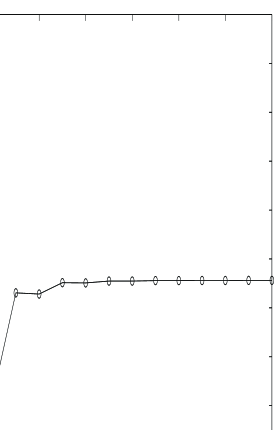
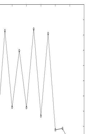
(a)                                                               (b)

FIG. 3.: $|{\cal R}_{11}|$ vs. $L$ for (a) $M=50$ and (b) $M=L$. Note that, as with the bound state problem, setting $M=L$ produces unsatisfactory results.

IV Results and Discussion

A Eigenenergies of the bound states

We first examine the dependence of the bound state energies on the parameter $s_{0}$, the length of the curved region of the tube. Figure 4 plots the momenta $\bar{k_{j}}$ corresponding to bound state eigenenergies against the angle of the circular arc $\theta$ $(=2\kappa s_{0})$ for curvature $\kappa=0.8$. Eigenenergies for both symmetric states and antisymmetric states are shown.

                                                                    

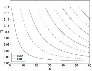
FIG. 4.: Plot of $\bar{k_{j}}$ vs. $\theta$, for $\kappa=0.8$.

The curved region introduces a term that behaves like an attractive finite square well potential with depth $\kappa^{2}/4$. Increasing the length of this curved region both lowers the energy of the ground state and allows for more excited states.

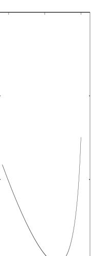
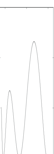
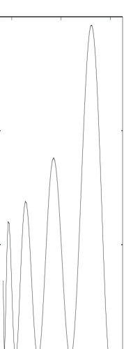
FIG. 5.: Plots of $\Delta(k)$ vs. $k$ for $\kappa=0.8$ and different $\theta$. Only symmetric states are considered. The minima correspond to $\bar{k_{j}}$ for odd values of $j$.

Figure 5 shows plots of the lowest eigenvalue of the matrix $\Xi$ as defined in §II.B against $k$, for curvature $\kappa=0.8$ and different values of the angle $\theta$. The minima on these graphs are candidate (symmetric) bound states provided $\bar{k}<\pi$, and correspond to points in Figure 4 along a line of fixed angle. As the angle increases, the number of eigenstates also increases.

In the limit $\theta\rightarrow\infty$, all the $\bar{k_{j}}$ approach the same value, which we will denote by $\bar{k}_{\infty}$. The value of $\bar{k}_{\infty}$ is that which corresponds to $\nu=0$ for any given curvature. To see this, note that in the limit $\theta\rightarrow\infty$, the external straight region becomes negligible (for bound states), and the internal curved region becomes very long. In this limit it becomes possible to accomodate wavefunctions with any number of nodes (in $s$) without introducing significant energy. The longitudinal wavefunction, $\cos\kappa\nu s$, (the antisymmetric case can be handled analogously) can oscillate any number of times over the range $-s_{0}<s<s_{0}$ contributing only $\kappa^{2}\nu^{2}$ to the energy. By choosing $\nu$ very small this contribution to the energy can be made negligible. A minute tuning of $\nu$ allows one to match the wavefunction to a falling exponential at $s=s_{0}$. Thus as $s_{0}\rightarrow\infty$ there are an infinite number of bound states accumulating at the value of $k$ corresponding to $\nu=0$. At any fixed very large $s_{0}$ there are also many other bound states at energies between $\bar{k}_{\infty}$ and $\pi$. The value of $\bar{k}_{\infty}$ is determined by solving the transcendental equation,

$$\left[Y_{0}\left(\frac{\bar{k}_{\infty}}{\kappa}\right)J_{0}\left(\frac{\bar{k}_{\infty}}{\kappa}(1-\kappa)\right)-J_{0}\left(\frac{\bar{k}_{\infty}}{\kappa}\right)Y_{0}\left(\frac{\bar{k}_{\infty}}{\kappa}(1-\kappa)\right)\right]=0.$$ (54)

This provides us with $\bar{k}_{\infty}(\kappa)$. As $\kappa\rightarrow 1$, $Y_{0}$ becomes singular in eq. (54). A careful analysis of the behavior at small $1-\kappa$ shows that the equation reduces to $J_{0}(\bar{k}_{\infty}(\kappa=1))=0$, which gives $\bar{k}_{\infty}(1)=2.405\dots$.[11]

Figure 6 plots the solution of eq. (54), $\bar{k}_{\infty}(\kappa)$ against $\ln(1-\kappa)$. As $\kappa\rightarrow 0$ $(\ln(1-\kappa)\rightarrow 0)$, the tube is straight and so $\nu=0$ corresponds to $k=\pi$, as expected. And as $\kappa\rightarrow 1$, $\bar{k}_{\infty}\rightarrow 2.405\dots$ as expected. It should be noted that the amount of binding increases dramatically as $\kappa\rightarrow 1$, a fact which necessitated our choice of $\ln(1-\kappa)$ as the independent variable in Fig. 6.

                                                                    

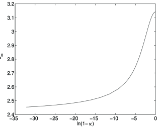
FIG. 6.: The value of $\bar{k}_{\infty}$ as a function of $\ln(1-\kappa)$.

Next we turn our attention to determining the angle at which the first (antisymmetric) bound excited state appears. We label the angles at which new bound states appear as $\bar{\theta_{1}}$, $\bar{\theta_{2}}$, etc. where $\bar{\theta_{1}}$ corresponds to the ground state and $\bar{\theta_{j}}$ $(j>1)$ to the $(j-1)^{th}$ excited state. For any $\kappa$, $\bar{\theta_{1}}$ is zero, since there exists a bound state for any tube with a curved region, no matter how short.

                                                                    

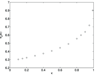
FIG. 7.: The angle $\theta$ at which the first antisymmetric bound state appears as a function of curvature $\kappa$. As $\kappa\rightarrow 0$, $\theta\rightarrow 2\pi$.

Figure 7 shows a plot of $\bar{\theta_{2}}(\kappa)$. As can be seen from the graph, $\bar{\theta_{2}}$ approaches $2\pi$ as $\kappa$ approaches zero. We can see that this must be the case by considering the one-channel approximation to the interior wavefunction, namely

$$\psi=\sin\pi y\sin\nu_{1}\kappa s.$$ (55)

It is sufficient to consider this approximation because in the limit that $\kappa\rightarrow 0$, the tube is very close to straight and thus the contributions from higher channels are negligible. In this limit, the problem reduces to that of a square well potential. The Schrödinger equation then requires

$$\nu_{1}^{2}\kappa^{2}-\frac{\kappa^{2}}{4}=k^{2}-\pi^{2}.$$ (56)

At the angle where the bound state first appears, $k=\pi$ so eq. (56) implies $\nu_{1}=\frac{1}{2}$. For a bound state to exist, the interior wavefunction ($\sin\nu_{1}\kappa s$) must be able to match to a falling exponential at the boundary $s=s_{0}$. The smallest value of $s_{0}$ at which this can occur is that which satisfies the condition $\nu_{1}\kappa s_{0}=\pi/2$. Recalling that $s_{0}=\theta/2\kappa$, we then have

$$\frac{\kappa}{2}\left(\frac{\theta}{2\kappa}\right)=\frac{\pi}{2}\Longrightarrow\theta=2\pi.$$ (57)

We note that as $\kappa$ is increased, the value of $\bar{\theta_{2}}$ also increases. This seems somewhat counter-intuitive, as we expect from the Schrödinger equation that higher curvature implies greater binding, so that the length of the curved region necessary to bind an excited state should decrease with large $\kappa$. This is indeed the case. However, we must recall that $\theta$ depends on $\kappa$ as well as $s_{0}$. For a fixed value of $\theta$, $s_{0}$ is much larger for small $\kappa$ than for large $\kappa$. Thus, the attractive potential acts over a much longer distance for small $\kappa$, and this effect overshadows the difference in binding energy due to differences in $\kappa$ alone.

B Scattering results

Previous workers have noted many features of the scattering problem, and we do not have any qualitatively new phenomena to add to their treatments.[8, 9] The primary features of interest to us are the rapid rise of $|{\cal T}_{11}|$ from threshold, the steady increase of the phase of ${\cal T}_{mm}$ in regions of energy away from thresholds, and finally, the dramatic fluctuations in ${\cal T}$ and ${\cal R}$ at energies just below thresholds. Our interest lies in understanding better the physical origins of these effects. These features are due to the presence of a bound state just below threshold, a steadily growing phase over a wide range of $k$, and weakly coupled quasibound states just below each channel threshold, respectively. The last of these provides an elegant example of a resonance manifesting itself as total destructive interference — a phenomenon familiar to particle physicists in the form of the sudden drop in the $\pi\pi\rightarrow\pi\pi$ $S$-wave cross section just below $\bar{K}K$ threshold, due to the presence of the $a_{0}$ resonance.[12]

We begin by examining $|{\cal T}_{11}|$ and $|{\cal R}_{11}|$ as functions of $k$. Figure 8 plots $|{\cal T}_{11}|^{2}$ and $|{\cal R}_{11}|^{2}$, the measures of transmitted and reflected flux, for $1\leq N\leq 3$ at fixed $\kappa=0.9$ and $\theta=\pi/2$.

                                                                    

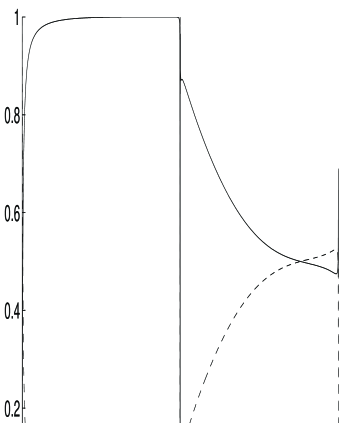
FIG. 8.: $|{\cal T}_{11}|^{2}$ (solid) and $|{\cal R}_{11}|^{2}$ (dashed) vs. $k/\pi$. Here $\kappa=0.9$, $\theta=\pi/2$.

Note that in the region where $N=1$ ($\pi\leq k<2\pi$), $|{\cal T}_{11}|^{2}+|{\cal R}_{11}|^{2}=1$. This is required by unitarity and serves as a check on our numerical calculations. We have checked that our ${\cal S}$-matrix remains unitary in the $N\times N$ case as well. As $k$ crosses the second threshold at $2\pi$ there is significant inelasticity into the newly open channel evidenced by the fact that $|{\cal T}_{11}|^{2}+|{\cal R}_{11}|^{2}<1$.

We also observe that at energies just below $N^{2}\pi^{2}$, the transmission amplitude in the highest open channel (${\cal T}_{N-1\,N-1}$) drops sharply almost to zero. We shall show that this and other rapid variations in ${\cal T}$ and ${\cal R}$ are manifestations of resonances related to the presence of quasibound states just below each new channel threshold. They are the energies at which we would find a bound state if all open channels were artificially closed.

It is difficult to figure out what is happening by considering $|{\cal T}|$ and $|{\cal R}|$ alone. We will learn much more by looking at the Argand diagrams for ${\cal T}$ and ${\cal R}$. The general characteristics will be illustrated by considering plots of ${\cal T}_{11}$ and ${\cal R}_{11}$ in the complex plane for $\pi<k<2\pi$ as shown in figure 9.

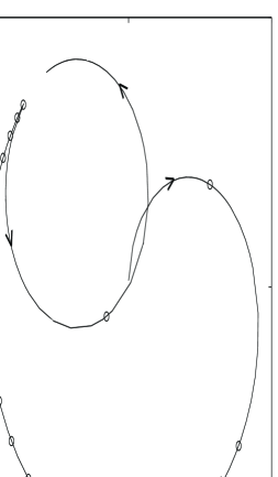
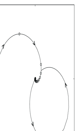
(a)                                                               (b)

FIG. 9.: Argand diagrams for (a) ${\cal T}_{11}$ and (b) ${\cal R}_{11}$ for the parameters $\kappa=0.9$, $\theta=\pi/2$, $\pi<k<2\pi$. Arrows indicate direction of increasing $k$; circles mark equal intervals in $k$.

${\cal R}_{11}$ and ${\cal T}_{11}$ are not independent when only one channel is open. Unitarity (${\cal S}^{\dagger}{\cal S}=1$) requires both $|{\cal T}_{11}|^{2}+|{\cal R}_{11}|^{2}=1$ and ${\rm Re}\,{\cal T}_{11}^{*}{\cal R}_{11}=0$. We can parameterize both by the modulus ($M$) and phase ($\phi$) of ${\cal T}_{11}$,

$${\cal T}_{11} = Me^{i\phi}$$ (58)

$${\cal R}_{11} = i\sqrt{1-M^{2}}e^{i\phi}$$ (59)

So it suffices to discuss the behavior of ${\cal T}_{11}$. According to Fig. (9), ${\cal T}_{11}$ vanishes at $k=\pi$. As $k$ increases, ${\cal T}_{11}$ rapidly executes a clockwise circle of radius $1/2$ in the complex plane until $|{\cal T}_{11}|\approx 1$ at a $k$ only slightly larger than $\pi$. Then ${\cal T}_{11}$ moves clockwise on the unit circle until suddenly, at a $k$ just below $2\pi$, ${\cal T}_{11}$ suddenly executes an almost complete counterclockwise circle of radius $1/2$. ${\cal T}_{11}$ briefly resumes its steady phase growth, until the second channel opens at $k=2\pi$ and ${\cal T}_{11}$ moves off the unit circle.

First consider the behavior near $k=\pi$. We know on general grounds that ${\cal T}_{11}=0$ and ${\cal R}_{11}=-1$ at threshold. Furthermore, we know that there is a symmetric bound state at an energy $k^{2}=\bar{k}_{1}^{2}=\pi^{2}-\varepsilon$. This must appear as a pole in ${\cal T}+{\cal R}$ at this energy. Since ${\cal S}$ must be unitary for any real $k^{2}$, ${\cal T}_{11}+{\cal R}_{11}$ must be of the form,

$${\cal T}_{11}+{\cal R}_{11}={k_{1}+i\varepsilon\over{k_{1}-i\varepsilon}}+f_{\sigma}(k)$$ (60)

where $k_{1}=\sqrt{k^{2}-\pi^{2}}$, and $f_{\sigma}(k)$ is a smoothly varying function of $k$ near $k=\pi$. There is no nearby antisymmetric bound state, so ${\cal T}_{11}-{\cal R}_{11}$ is a smooth function of $k$,

$${\cal T}_{11}-{\cal R}_{11}=f_{\alpha}(k)$$ (61)

near $k=\pi$. Comparing with the threshold behavior, ${\cal T}_{11}=0$ and ${\cal R}_{11}=-1$, we see that $f_{\sigma}(\pi)=0$ and $f_{\alpha}(\pi)=1$. Combining all these results we obtain,

$${\cal T}_{11} = e^{i\phi}\cos\phi$$ (62)

$${\cal R}_{11} = ie^{i\phi}\sin\phi\quad{\rm where}$$ (63)

$$\tan\phi \equiv {\varepsilon\over k_{1}}$$ (64)

At threshold, $\phi=\pi/2$, and as $k$ increases, $\phi$ drops rapidly to zero over an interval scaled by $\varepsilon$. Eqs. (LABEL:thresh) parameterize a semicircle of radius $1/2$ centered at ${\cal T}_{11}=1/2$, which ${\cal T}_{11}$ executes as $k_{1}$ grows from zero to a value greater than $\varepsilon$. The speed at which ${\cal T}_{11}$ moves measures $\varepsilon$, by the formula

$$\varepsilon=ik_{1}\left({1\over{\cal T}_{11}}-1\right)$$ (66)

For $k_{1}\gg\varepsilon$ the conditions of the small $\kappa$ approximation discussed in §II are satisfied, provided $\kappa$ is small. Thus we expect to find ${\cal R}_{11}\approx 0$ and ${\cal T}_{11}={\cal T}_{11}^{0}\times\exp(-ik_{1}\theta/2)$. We verify this by comparing the rate of change of the argument of ${\cal T}_{11}$ with the small $\kappa$ prediction, $d\arg{\cal T}_{11}/dk_{1}=-\theta/2$. So in the range where the approximation is valid, we expect that the graph of the phase angle $\phi$ of ${\cal T}$ will be linear with respect to $k_{1}$, with a slope equal to half the angle subtended by the curved region of the tube. Computing ${\cal T}_{11}$ for $4.0<k_{1}<5.0$ with $\kappa=0.001$ and $\theta=\pi/2$, a range and curvature for which the small $\kappa$ approximation is valid, we have found $d\arg{\cal T}_{11}/dk_{1}\approx-\pi/4=-\theta/2$, which confirms that this relation is indeed satisfied.

Finally we turn to the dramatic behavior of ${\cal T}$ and ${\cal R}$ near channel thresholds. It is clear from Fig. (9) that ${\cal T}_{11}$ resonates (i.e. it rapidly executes a counterclockwise circle in the complex plane[13]) at the energy where $|{\cal T}_{11}|$ drops precipitously to zero. This behavior is indicative of a pole in the complex $k^{2}$ plane just below the real axis. The pole appears in ${\cal T}_{11}+{\cal R}_{11}$ because the quasibound state is symmetric in $s$. ${\cal T}_{11}-{\cal R}_{11}$ is smooth over this region in $k$. If we denote the pole location as $q_{1}-i\gamma_{1}$, where $q_{1}\lessapprox 2\pi$ and $\gamma_{1}$ is small and positive (by causality). Then in the neighborhood of the pole,

$${\cal T}_{11}+{\cal R}_{11}={k_{1}-q_{1}-i\gamma_{1}\over k_{1}-q_{1}+i\gamma_{1}}+\ldots,$$ (67)

where $\ldots$ denotes other, smooth terms in ${\cal T}_{11}+{\cal R}_{11}$. Combining this with a smooth form for ${\cal T}_{11}-{\cal R}_{11}$ we see that ${\cal T}_{11}$ executes a counterclockwise circle of radius $1/2$ in the complex $k$-plane as $k$ passes over the pole. Just before the vicinity of the pole, ${\cal T}_{11}$ lay nearly on the unitarity circle, $|{\cal T}_{11}|\approx 1$. The only way that it could rapidly execute a counterclockwise circular path consistent with unitarity is if the resonant circle is tangent to the unitarity circle. [Otherwise ${\cal T}_{11}$ would have to pass outside the unit circle at some point on its circular path.] Since the radius of the resonance circle is $1/2$, the (tangent) resonant circle must pass through the origin. Thus $|{\cal T}_{11}|$ must vanish in the near vicinity of the quasibound state as observed by Ref. [9], and shown in Fig. (9).

The basic structure of ${\cal T}_{11}$ and ${\cal R}_{11}$ can be seen in the scattering coefficients for higher channels. As we observe in figure 10 for $N=2$, ${\cal T}_{12}$ and ${\cal T}_{22}$ follow the same pattern. For $k_{2}=\sqrt{k^{2}-4\pi^{2}}$ just above zero, ${\cal T}$ executes rapid clockwise motion as a result of the pole located near $k=\pi$. This is followed by smooth phase growth until $k$ reaches the quasi-bound state just under the $N=3$ threshold, at which time it executes the rapid counterclockwise circle in the complex plane characteristic of an elastic resonance.

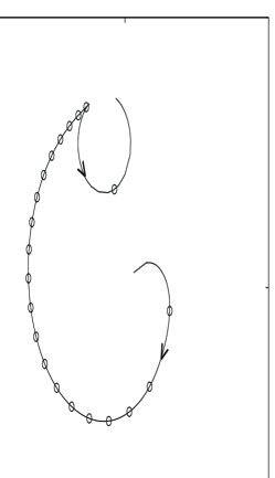
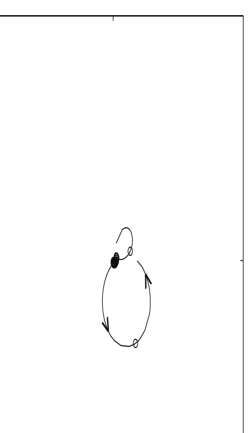
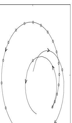
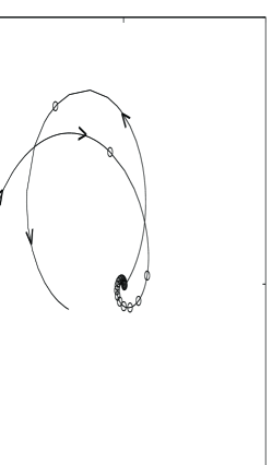
FIG. 10.: Argand diagrams for ${\cal T}_{12}={\cal T}_{21}$, ${\cal T}_{22}$, ${\cal R}_{12}={\cal R}_{21}$, and ${\cal R}_{22}$ for the range $2\pi<k<3\pi$. The same basic structure is observed as for the coefficients in the $N=1$ case.

Our conclusion from this exercise is that the behavior observed in Fig. 9 is characteristic of scattering in bent tubes. The bound states, quasibound states and regions of smooth phase growth are robust properties of these systems. They do not depend specially on our choice of a circular geometry which facilitated our numerical calculations. Perhaps the most interesting observation is the appearance of violent fluctuations in transmission and reflection properties of bent tubes in the vicinity of channel thresholds. The fluctuations occur over very narrow intervals in energy (the resonances are narrow), so low resolution experiments would quite likely fail to detect them. On the other hand, careful experiments using, for example, microwave radiation in waveguides, should see these rapid fluctuations in response associated with the opening of channel thresholds in which quasibound states occur.

REFERENCES

- [1] H. Jensen and H. Koppe, Ann. Phys. (NY) 63 (1971) 586.
- [2] M. Kügler and S. Shtrikman, Phys. Rev. D37 (1988) 934;M. Ikegami, Y. Nagaoka, S. Tagaki, T. Tanzawa, Prog. Theor. Phys. 88 (1992) 229.
- [3] F. Lenz, T. J. Londergan, E. Moniz, R. Rosenfelder, M. Stingl, and K. Yazaki, Ann. Phys. (NY) 170 (1986) 65; J. P. Carini, J. T. Londergan, K. Muller, and D. P. Murdock, Phys. Rev. B48 (1993) 4503.
- [4] For a review of applications to condensed matter physics, see C. W. J. Beenakker and V. van Houten in Solid State Physics editedby H. Ehrenreich and D. Turnbull (Academic, New York, 1991).
- [5] R. L. Schult, D. G. Ravenhall and H. W. Wyld, Phys. Rev. B39 (1989) 5476.
- [6] P. Exner and P. Seba, J. Math. Phys. 30 (1989) 2574 and references therein.
- [7] J. Goldstone and R. L. Jaffe, Phys. Rev. B45 (1992) 14,100.
- [8] C. S. Lent, Appl. Phys. Lett. 56 (1990) 2554.
- [9] F. Sols and M. Macucci, Phys. Rev. B 41 (1990) 11,887.
- [10] F. E. Low, Symmetries and Elementary Particles, (Gordon and Breach, New York, 1967).
- [11] K. Lin, MIT Undergraduate Thesis, unpublished, 1995.
- [12] R. L. Jaffe and F. E. Low, Phys. Rev. D19 (1979) 2105.
- [13] M. L. Goldberger and K. M. Watson, Collision Theory (Wiley, New York, 1964).