Degenerate Bose liquid in a fluctuating gauge field

Abstract

We study the effect of a strongly fluctuating gauge field on a degenerate Bose liquid, relevant to the charge degrees of freedom in doped Mott insulators. We find that the superfluidity is destroyed. The resulting metallic phase is studied using quantum Monte Carlo methods. Gauge fluctuations cause the boson world lines to retrace themselves. We examine how this world-line geometry affects the physical properties of the system. In particular, we find a transport relaxation rate of the order of 2$k_{\rm B}T$, consistent with the normal state of the cuprate superconductors. We also find that the density excitations of this model resemble that of the full $t$-$J$ model.

Much attention has been focused on the normal state of the cuprate superconductors, which exhibit non-Fermi-liquid behavior over a wide range of temperatures. For instance, the resistivity is linear in temperature up to 1000K in optimally doped La_2-xSr_xCuO₄. Optical conductivity measurements show a Drude peak with a scattering rate $1/\tau_{\rm tr}$ of the order of $2k_{\rm B}T$. The Hall resistivity is suppressed relative to the classical value $B/nec$ with a $1/T$ temperature dependence. The magnetoresistance is also anomalous in that it violates Köhler’s rule [1]. Anderson [2] emphasized the role of antiferromagnetic correlations in these doped Mott insulators, and introduced the idea of a resonating-valence-bond (RVB) state, which pointed to spin-charge separation at low energies. In a gauge-theoretic formulation [3, 4], charge and spin are represented by bosonic holes (“holons”) and neutral spin-half fermions (“spinons”) interacting via a fluctuating U(1) gauge field.

In this Letter, we study the bosonic holons as a two-dimensional Bose liquid in the presence of a fluctuating perpendicular magnetic field. Physically, the interaction of a boson with the transverse gauge field, ${\bf a}$, describes the motion of a vacancy in a spin background with fluctuating quantization axes [4]. The flux, $\Phi_{\bf r}$, due to this gauge field represents the chirality of the spins around the plaquette ${\bf r}$. We treat the gauge field in a quasistatic limit (which we justify below) where we consider an annealed average over static flux distributions which scatter the bosons elastically. (In contrast, Wheatley and coworkers [5] emphasized the dissipative part of the scattering.) In the regime of strong gauge fluctuations, the boson world lines attempt to retrace themselves [6, 7], so that this system can be regarded as a bosonic analogue of the Brinkman-Rice problem [8, 9]. We find that superfluidity is destroyed even when there is significant exchange among the bosons. This results in a degenerate Bose metal with interesting charge dynamics such as a Drude peak in the optical conductivity, consistent with the experimental scattering rate of $2k_{\rm B}T$.

We believe that our results for the boson model are relevant to the charge dynamics of the $t$-$J$ model where electrons hop (with matrix element $t_{0}$) under a constraint of no double occupancy and with a nearest-neighbor spin exchange energy $J$. In the gauge theory for the uniform RVB state in this model [3, 4], gauge fluctuations at weak coupling are described by the correlator $D({\bf k},\omega_{n})=\langle|a_{\perp}({\bf k},\omega_{n})|^{2}\rangle=(\chi k^{2}+\gamma|\omega_{n}|/k)^{-1}$, where $\chi$ is the orbital susceptibility of the spinon fluid, $\gamma$ is the Landau damping coefficient, $\omega_{n}=2\pi n/\beta$ and $\beta=1/k_{\rm B}T$. We can see that these fluctuations are overdamped with a relaxation time which diverges as $1/k^{3}$. This justifies the quasistatic limit, i.e. $D({\bf k},\omega_{n})\rightarrow D({\bf k},\omega_{n}=0)\,\delta_{n,0}$, as a first approximation to the long-wavelength physics of this system. The flux distribution is then spatially uncorrelated: $\langle\Phi_{\bf r}\Phi_{\bf r^{\prime}}\rangle=(b^{2}/\beta\chi)\,\delta_{{\bf r},{\bf r^{\prime}}}$ where $b$ is the lattice spacing. Note that, although $\langle\Phi^{2}\rangle$ decreases with temperature, the typical flux through a plaquette is of the order of a flux quantum ($\Phi_{0}=hc/e$) in the temperature range where the cuprates are normal: $T/J>T_{\rm c}/J\simeq 0.1$. A simple estimate, using a Fermi gas to calculate $\chi$, gives us $\langle\Phi^{2}\rangle^{1/2}\sim(3T/\pi J)^{1/2}\Phi_{0}>0.25\Phi_{0}$. A more detailed calculation gives $\langle\Phi^{2}\rangle^{1/2}\simeq 0.5\Phi_{0}$ for $T>0.3J$ [10]. In the presence of such strong fluctuations, the behavior of the holons should be insensitive to the detailed value of $\langle\Phi^{2}\rangle$ and we will work with a large but constant $\langle\Phi^{2}\rangle$.

To be precise, we study in this paper the model described by the imaginary-time action: $S=S_{\rm B}+S_{\rm G}$ where

$$S_{\rm B} = \int_{0}^{\beta}\!\left(\sum_{i}b_{i}^{\dagger}\frac{\partial b_{i}}{\partial\tau}-H_{\rm B}(\tau)\right)d\tau$$ (1)

$$S_{\rm G} = \frac{1}{2\beta L^{2}}\sum_{{\bf k}}D^{-1}({\bf k},0)|a({\bf k},0)|^{2}=\sum_{\bf r}\frac{\Phi_{\bf r}^{2}}{2\langle\Phi^{2}\rangle}$$ (2)

$$H_{\rm B} = -t\sum_{\langle ij\rangle}(e^{ia_{ij}}b_{i}^{\dagger}b_{j}+{\rm h.c.})+\frac{U}{2}\sum_{i}n_{i}(n_{i}-1)$$ (3)

with $U/t\gg 1$ on an $L\times L$ lattice. The partition function $Z$ for $N$ particles is obtained by summing over all periodic configurations of boson world lines $\{{\bf x}_{\alpha}(\tau)\}$ ($0<\tau<\beta,\alpha=1,\dots,N$) and all flux distributions:

$$Z=\int\!\!{\cal D}{\bf a}\prod_{\alpha=1}^{N}\!\int\!\!\frac{{\cal D}{\bf x}_{\alpha}}{N!}e^{-S_{\rm G}[{\bf a}]-i\sum_{\alpha}\int_{0}^{\beta}\!\!{\bf a}\cdot d{\bf x}_{\alpha}\,-\,S_{\rm B}^{0}[\{{\bf x}\}]}$$ (4)

where $S_{\rm B}^{0}$ is the action for the world lines in the absence of a magnetic field. The path integration includes world-line configurations where the final boson positions, ${\bf x}_{\alpha}(\beta)$, are related to the initial ones, ${\bf x}_{\alpha}(0)$, by a permutation of the particle labels, $\alpha$. In other words, exchange may give rise to world-line loops containing more than one boson. Performing the annealed average over the Gaussian flux distribution, we obtain an effective action for the bosons alone: $S_{\rm eff}=S^{0}_{\rm B}+S_{2}$ with

$$S_{2}={\frac{1}{2\beta}}\sum_{\alpha\alpha^{\prime}}\int_{0}^{\beta}\!\!\!\int_{0}^{\beta}\!\!{\tilde{D}}({\bf x}_{\alpha}(\tau)-{\bf x}_{\alpha^{\prime}}(\tau^{\prime}))\,{\bf\dot{x}}_{\alpha}\!\cdot\!{\bf\dot{x}}_{\alpha^{\prime}}\,d\tau\,d\tau^{\prime}$$ (5)

where $\tilde{D}({\bf x})=L^{-2}\sum_{{\bf k}\neq 0}D({\bf k},0)e^{i{\bf k\cdot x}}$ is proportional to the Green’s function of the lattice Laplacian. The k=0 contribution is excluded because it represents a global change of gauge for ${\bf a}$.

The nonlocal current interaction $S_{2}$ can be better understood in terms of the winding of the boson world lines around the plaquettes of the lattice. For instance, on an infinite plane, the phase factor in Eq. (4) is $\exp(-2\pi i\sum_{\bf r}w_{\bf r}\Phi_{\bf r}/\Phi_{0})$ where $w_{\bf r}$ is the total winding number of all the world lines around plaquette ${\bf r}$. Averaging over the flux distribution gives $S_{2}=(2\pi^{2}\langle\Phi^{2}\rangle/\Phi_{0}^{2})\sum_{\bf r}w^{2}_{\bf r}$. To be more careful, we should restrict ourselves to distributions with zero total flux: $\sum_{\bf r}\Phi_{\bf r}=0$, which means that we should replace $\sum_{\bf r}w^{2}_{\bf r}$ by $\sum_{\bf r}w^{2}_{\bf r}-(\sum_{\bf r}w_{\bf r})^{2}/L^{2}$ in the above formula. This winding-number sum has been termed the “Amperean area” of the world-line configuration [7]. We see that, in the presence of strong gauge fluctuations, the partition function is dominated by paths with zero Amperean area. These are “retracing paths” where each traversal of a link on the lattice is retraced in the opposite direction at some point in time [8, 9] (Fig. 1a), and so their contribution to $Z$ is unaffected by the average over the gauge field. On the other hand, averaging causes destructive interference for non-retracing paths.

It is in fact more efficient to enumerate $S_{2}$ in terms of winding numbers. To do so under the periodic boundary conditions of a torus, we have to extend the definition of $w_{\bf r}$. This can be done for world-line configurations which do not have a net wrapping around the torus in either spatial direction. A suitable definition (i.e. one which preserves Stokes’ theorem, $\oint{\bf a}({\bf x})\cdot d{\bf x}=\sum_{\bf r}w_{\bf r}\Phi_{\bf r}$, in the case of zero total flux) is: $w_{\bf r}=\tilde{\Phi}^{-1}\oint[{\bf a}^{0}_{\bf r}({\bf x})-{\bf a}^{0}_{\bf R}({\bf x})]\cdot d{\bf x}$, where ${\bf a}^{0}_{\bf r}({\bf x})$ is the vector potential at ${\bf x}$ due to a test flux $\tilde{\Phi}$ placed at plaquette ${\bf r}$, and ${\bf R}$ is an arbitrary reference plaquette. Geometrically, this picks ${\bf R}$ to be on the “outside” of any loop on the torus.

We now turn to world-line configurations which have a net wrapping around the torus. These configurations are signals of superfluidity. Indeed, the superfluid density $n_{\rm s}$ (per site) is given by[11]: $n_{\rm s}=\langle{\bf W}^{2}\rangle/4\beta t$, where ${\bf W}=(W_{x},W_{y})$ are the total numbers of times the world lines wrap around the torus in the $x$ and $y$ directions respectively. In our problem, these paths pick up the random Aharonov-Bohm phases which thread the torus, and so should be suppressed after averaging over the gauge field. For instance, Eq. (5) gives $S_{2}=(W_{y}^{2}/2\beta)\sum_{k_{x}\neq 0,k_{y}=0}D({\bf k},0)\sim W_{y}^{2}\langle\Phi^{2}\rangle L^{2}/\Phi_{0}^{2}$ for a straight-line path which wraps around the system $W_{y}$ times in the $y$-direction. In general, one can evaluate $S_{2}$ for a world-line configuration with total wrapping numbers ${\bf W}=(W_{x},W_{y})$ by decomposing it into a reference straight-line path with the same ${\bf W}$ and a set of world lines with no net wrapping (Fig. 1b-c). Terms in Eq. (5) involving the non-wrapping part only can then be evaluated as above, while terms involving the wrapping reference path must be evaluated using Eq. (5) directly. Thus, we see that any wrapping configuration would give a positive contribution to $S_{2}$ of order ${\bf W}^{2}L^{2}$, and so should be strongly suppressed in the partition function. We therefore argue that, for fixed $\langle\Phi^{2}\rangle$, superfluidity is destroyed at all temperatures as $L\to\infty$.

FIG. 1.: (a) A retracing world line path projected onto the $xy$ plane. (b) A wrapping path. (c) Decomposition of (b) into a reference path and a non-wrapping path.

To establish the existence of this degenerate Bose metal and to characterize this phase, we have performed a path-integral quantum Monte Carlo simulation [12] of this effective action with $U/t=4$ at 25% boson filling with periodic boundary conditions. $S_{2}$ is evaluated using the prescription described above. Note that $S_{2}$ is real so that there is no sign problem in the path integration. Each Monte Carlo step involves the reconstruction of the world lines, $\{{\bf x}_{\alpha}(\tau)\}$, for all the particles ($\alpha=1,\dots,N$) in an interval of imaginary time. To ensure quantum exchange, we insist that each accepted configuration differs from the previous one by a pair exchange. Since we are interested in the regime of strong flux fluctuations, we use a fine-grained discretization in the time direction ($\Delta\tau\leq 0.1/t$) so that deviations from a retracing path can be sampled correctly. A reasonably large number of imaginary-time points is also desirable for our analytic continuation of the dynamical quantities of interest. These factors limit our simulations to $T>0.1t$.

We have measured the superfluid fraction at $T=t/6$ for a range of flux variances and for system sizes up to 7$\times$7 lattices (Fig. 2). In the absence of gauge fields, the system has a Kosterlitz-Thouless transition at $T_{\rm KT}\simeq t$ so that the superfluid fraction is nearly unity at $T=t/6$. There is a threshold $\langle\Phi^{2}\rangle_{\rm c}$ beyond which the superfluid density is exponentially small. Our arguments suggest that $\langle\Phi^{2}\rangle_{\rm c}$ vanishes as $1/L^{2}$ as $L\rightarrow\infty$ (Fig. 2 inset).

FIG. 2.: Superfluid fraction as a function of flux variance $\langle\Phi^{2}\rangle$ and system size $L$ at $\beta t=6$ ($t\Delta\tau=0.05$). Inset: a scaling plot suggests that superfluidity vanishes at $\langle\Phi^{2}\rangle_{\rm c}L^{2}/\Phi_{0}^{2}\simeq 8$.

Although our system has no superfluid response, it may still have diverging correlation lengths and diamagnetic response as $T\rightarrow 0$, as in the classical analogue of this problem where the gauge field screens the vortex-antivortex binding potential and the Kosterlitz-Thouless phase is destroyed. Such divergences do not happen for strong gauge fluctuations. As already mentioned, boson paths are retracing in this limit and so, the system has no linear response to external magnetic fields. Indeed, the diamagnetic susceptibility is too small to measure in our simulation. This insensitivity to external fields is consistent with the observation that the Hall resistance is suppressed from its classical value, and that the magnetoresistance violates Köhler’s law[1].

Another consequence of the retracing of paths is that the system might form dense aggregates. Feigelman et al.[13] showed that this phase separation might occur in the dilute limit. However, we have not found evidence for inhomogeneity or strong density fluctuations in our regime of moderate density and strong on-site repulsion.

We now turn to the transport properties of this system. We use $\langle\Phi^{2}\rangle=0.5\Phi_{0}^{2}$ to ensure that we work in the regime of strong gauge fluctuations, where the world-line configuration have zero Amperean area. Using the gauge-invariant current ${\bf j}(\tau)=\sum_{\alpha}[{\bf x}_{\alpha}(\tau+\Delta\tau)-{\bf x}_{\alpha}(\tau)]/\Delta\tau$, we have measured the current correlation function to an accuracy of 0.3-0.9%. Through analytic continuation and the Kubo formula, the a.c. conductivity $\sigma(\omega)$ is related to the current correlation function by

$$-\frac{1}{L^{2}}\langle j_{x}(\tau)j_{x}(0)\rangle=\int_{-\infty}^{\infty}\!\!\frac{\omega e^{-\omega\tau}\sigma(\omega)}{1-e^{-\beta\omega}}\frac{d\omega}{\pi}$$ (6)

for $\tau\neq 0$. We have performed this analytic continuation numerically using maximum entropy techniques [14]. Using the kinetic energy $\langle K\rangle$, we can check, to an accuracy of 3%, the sum rule: $\int_{0}^{\infty}\sigma(\omega)d\omega=-\pi\langle K\rangle/4L^{2}$. For the lowest temperatures ($T<0.4t$), we worked at fixed $\Delta\tau$ and $\beta t/L^{z}$ with $z=2$ to minimize finite-size effects [15].

FIG. 3.: Optical conductivity for 6x6 lattice at $\beta t=$ 9,6,4,2,1,0.5. Inset: kinetic energy, proportional to spectral weight. Dashed line (BR) denotes Brinkman-Rice band edge.

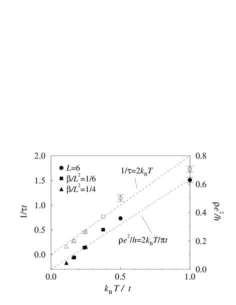
FIG. 4.: Transport. Resistivity (solid symbols) and scattering rate (hollow symbols) as a function of temperature. Scattering rate is deduced using the half-height of $\sigma(\omega)$.

We find that $\sigma(\omega)$ consists of a single Drude-like peak, which sharpens as the temperature is lowered (Fig. 3). The width of the peak gives us the transport scattering rate $1/\tau_{\rm tr}$. We find a temperature dependence consistent with: $1/\tau_{\rm tr}=\zeta k_{\rm B}T$ with $\zeta=1.8-2$. (Fig. 4). The resistivity $\rho$, given by the peak height, is consistent with a linear temperature dependence of $\rho e^{2}/h=(1/2\pi n_{0})k_{\rm B}T/t$ for $T<2t$, (Fig. 4), where $n_{0}$ is the boson number density. We estimate a statistical error of 5% for $\rho$ by examining fluctuations due to deviations in the current correlation function [16]. (There are also systematic errors due to the smoothing of structures.) There appears to be a systematic deviation from the linear-$T$ behavior below $T=0.3t$. This deviation is stronger for $\rho$ than for $1/\tau_{\rm tr}$. The difference can be attributed to the $T$-dependence of the weight under the conductivity peak. Since we only have one peak which exhausts the sum rule, this spectral weight is proportional to $-\langle K\rangle$. As $T$ decreases, $\langle K\rangle/N$ drops below the band edge of $-2\sqrt{3}t$ for the single-particle problem [8] and approaches remarkably close to $-4t$ per particle (Fig. 3 inset).

When we examine the paths, we find that the world-line loops span increasing number of periods in imaginary time as the temperature is lowered, indicating strong particle exchange below $T=0.5t$. As $T$ is reduced further, different loops begin to retrace each other. Thus, the transport properties shown in Fig. (4) are clearly characteristic of a quantum Bose system. This should be contrasted with the Brinkman-Rice result [8] for $k_{\rm B}T\gg t$, where the spectral weight decreases as $\langle K\rangle\sim T^{-1}$, and $1/\tau_{\rm tr}$ begins to saturate to a constant. This gives a linear-$T$ resistivity which clearly has a different physical origin from that shown in Fig. 4.

Our resistivity is in agreement, to within a factor of 2, with Jaklič and Prelovšek [17] who provided an approximate diagonalization of the $t$-$J$ model on 4$\times$4 lattices. They also find a Drude peak of width $\sim 2k_{\rm B}T$. In addition, they found a broad background which may be interpreted with a frequency-dependent scattering rate. This is absent in our boson model. This could be due to the absence of fermion degrees of freedom or our neglect of gauge-field relaxation.

FIG. 5.: Dynamic structure factor. Solid lines: our results for 6$\times$6 lattice at $\beta t=6$ with $t=0.9t_{0}$. Dashed lines: $tJ$ model with 4 holes in an 18-site cluster with $t_{0}/J=2.5$ [18].

Finally, we examine the dynamic structure factor $S({\bf q},\omega)$, related to the density correlation function by:

$$\frac{1}{L^{2}}\langle n_{\bf q}(\tau)n_{-\bf q}(0)\rangle=\!\int_{0}^{\infty}\!\!\!\!(e^{-\tau\omega}\!+\!e^{-(\beta-\tau)\omega})S({\bf q},\omega)d\omega$$ (7)

where $n_{\bf q}(\tau)=\sum_{\alpha}e^{i{\bf q\cdot x_{\alpha}(\tau)}}$. This should be relevant to electron energy loss experiments. The loss of long-ranged phase coherence means that the structure factor does not sharp phonon peaks as in the superfluid phase. For fixed ${\bf q}$, $S({\bf q},\omega)$ has a broad peak as function of $\omega$. For ${\bf q}$ in the ($\pi,\pi$) direction, these peaks coincide remarkably with features found in the exact-diagonalization study of Eder et al. [18] at a similar hole density (Fig. 5), after a moderate rescaling to $t$ by a factor of 0.9. On the other hand, our results differ from those of Eder et al. in the ($\pi,0$) direction. These authors found two peaks in the structure factor whereas we find only one.

In summary, we have studied a degenerate Bose system which is metallic due to elastic scattering with random gauge fields. We have demonstrated that many features of this model, such as the longitudinal transport time, indeed mimic the behavior of the full $t$-$J$ model and the normal state of the cuprate superconductors.

We are indebted to Wolfgang von der Linden for sending us his maximum-entropy program. We would also like to thank X.G. Wen and S.M. Girvin for useful discussions. This work was supported by the NSF MRSEC program (DMR 94-0034), EPSRC/NATO (DKKL), and NEC (DHK).

REFERENCES

- [1] For a review, see N.P. Ong, Y.F. Yan and J.M. Harris, CCAST Symposium on High- Superconductivity and the C60 Family, Beijing 1994 (Gordon and Breach, 1995)
- [2] P.W. Anderson, Science 235, 1196 (1987).
- [3] L.B. Ioffe and A.I. Larkin, Phys. Rev. B 39, 8988 (1989).
- [4] N. Nagaosa and P.A. Lee, Phys. Rev. Lett. 64, 2450 (1990); Phys. Rev. B 45, 966 (1992).
- [5] J.M. Wheatley, Phys. Rev. Lett. 67, 1181 (1991).
- [6] N. Nagaosa and P.A. Lee, Phys. Rev. B 43, 1233 (1991).
- [7] G. Gavazzi, J.M. Wheatley and A.J. Schofield, Phys. Rev. B 47, 15170 (1993).
- [8] W.F. Brinkman and T.M. Rice, Phys. Rev. B 2, 1324 (1970).
- [9] R. Oppermann and F. Wegner, Z. Phys. B 34, 327 (1979).
- [10] R. Hlubina, W.O. Putikka, T.M. Rice and D.V. Khveshchenko, Phys. Rev. B, 46, 11224 (1992).
- [11] E.L. Pollock and D.M. Ceperley, Phys. Rev. B 36, 8343 (1987); D.M. Ceperley and E.L. Pollock, ibid. 39, 2084 (1989).
- [12] N. Trivedi, “Computer Simulations in Condensed Matter Physics V”, eds. D. P. Landau et al., (Springer Verlag, Heidelberg, Berlin, 1993).
- [13] M.V. Feigelman, V.B. Geshkenbein, L.B. Ioffe and A.I. Larkin, Phys. Rev. B 48, 16641 (1993).
- [14] J.E. Gubernatis et al., Phys. Rev. B 44, 6011 (1991); W. von der Linden, Appl. Phys. A 60, 155 (1995).
- [15] X.G. Wen, Phys. Rev. B 46, 2655 (1992).
- [16] M. Jarrell, J.E. Gubernatis and R.N. Silver, Phys. Rev. B 44, 5347 (1991).
- [17] J. Jaklič and P. Prelovšek, Phys. Rev. B 52, 6903 (1995).
- [18] R. Eder, Y. Ohta and S. Maekawa, Phys. Rev. Lett. 74, 1241 (1995).