Abstract

We investigate Bethe Ansatz equations for the one-dimensional spin-$\frac{1}{2}$ Heisenberg XXX chain with a special interest in a finite system. Solutions for the two-particle sector are obtained. The ground state in antiferromagnetic case has been analytically studied through the logarithmic form of Bethe Ansatz equations.

1 Introduction

This paper is devoted to the study of Bethe Ansatz equations (BAE) for the isotropic spin-$\frac{1}{2}$ Heisenberg chain. The model describes interacting spins, situated on the sites of a periodic lattice $N$. There has been a profound development in physical interest on the thermodynamical properties of their solutions. In recent years a strong increase of mathematical attention on this subject arises from the study of integrable systems via quantum inverse scattering method. In most cases the results obtained are mainly concerned with the lattice size $N$ tending to infinity. However the finite-size problems, or the finite-size corrections, should be of mathematical interest, as well as essential to the understanding of BAE, which is the basis for all exact solutions of electronic models in one dimension. We intend to investigate here the finite-size BAE for Heisenberg XXX model in a rigorous mathematical way, which will serve as a standard theory for our subsequent works on quantum integrable systems.

In his remarkable works [1], Baxter discovered a link between the quantum spin models and transfer matrices of 2-dimensional statistical lattice models. The quantum inverse scattering method [8] provides a natural understanding of the role of Bathe Ansatz in the problem of spectrum of model Hamiltonians. For Heisenberg XXX Hamiltonian, Bethe vectors have some special characteristic properties: they are eigenvectors of of the corresponding transfer matrices with polynomials as the eigenvalues, and also the highest weight vectors for the global $sl_{2}$-symmetry of the Hamiltonian. In the investigation of solutions of BAE in the large $N$ limit, there is one fundamental assumption, the so-called string hypothesis (Takahashi [7]). We observe that a certain feature of these string structures can be understood through BAE, while the counting of states [9] based on this string hypothesis remains still valid for the 2-particle sector of any finite system $N$. The analytical solutions for sectors other than two particles are hard to obtain except a very small size, e.g. $N=6$. However for the ground state, one can study the problem by analysing the corresponding logarithmic form equation, where the fixed point theory can be used for the existence of solutions. The uniqueness of the ground state solution should be mathematically expected, but only strong indication can be obtained here. Such program is now under progress and partial results are promising.

The organization of this paper is as follows. In Section 2, we recall necessary definitions in the theory of quantum integrable systems [5] and give various characterizations of Bethe roots for Heisenberg XXX model. In Section 3, Bethe roots as $N\rightarrow\infty$ are discussed, and the string structure for a large $N$ is derived from BAE. In Section 4, we study some problems on Heisenberg XXX model of a finite lattice size. Here the BAE for the two-particle sector is solved analytically, and mathematical structures of BAE on the ground state in antiferromagnetic case, as well as the equivalent equation for its logarithmic form, are discussed. We establish rigorously the existence of ground state via the fixed point theory, and also the uniqueness of the solution for a small $N$. In Section 5, we present an illuminating ( but not a mathematically rigorous ) argument on the uniqueness of ground state for a large finite system. We have written this note in a mathematical style, and hope that in process it would not be much difficult to read for both mathematicians and theoretical physicians.

2 Characterizations of Bethe States

The Hamiltonian of Heisenberg XXX model is given by

$$H_{\rm XXX}=-\frac{J}{4}\sum_{n=1}^{N}(\sigma_{n}^{1}\sigma_{n+1}^{1}+\sigma_{n}^{2}\sigma_{n+1}^{2}+\sigma_{n}^{3}\sigma_{n+1}^{3}-1)\ ,\ \ \ \ J\in\hbox{IR}\ .$$

Here $\sigma^{j}$’s are Pauli matrices. In this paper, we shall always assume the size $N$ to be even with the periodic boundary condition ( $N+1\equiv 1$) . The operator $H_{\rm XXX}$ acts on the Hilbert space of physical states $\hbox{IH}_{N}$,

$$\hbox{IH}_{N}=\bigotimes_{n=1}^{N}h_{n}\ ,\ \ \ \ h_{n}:=\,\hbox{IC}^{2}\ \mbox{ for \ all \ }\ \ n.$$

The link between the above quantum XXX system and a 2-dimensional statistical lattice model is described as follows [1] [5]. Define the operators of $\,\hbox{IC}^{2}\otimes h$

$$\begin{array}[]{ll}R(\lambda)=&\left(\begin{array}[]{cc}\lambda\sigma^{4}+\frac{i}{2}\sigma^{3}&i\sigma^{-}\\ i\sigma^{+}&\lambda\sigma^{4}-\frac{i}{2}\sigma^{3}\end{array}\right)\ ,\ \ \ \ \sigma^{\pm}=\frac{\sigma^{1}\pm i\sigma^{2}}{2}\ ,\ \lambda\in\,\hbox{IC}\ ,\end{array}$$

with the first factor $\,\hbox{IC}^{2}$ as the auxiliary space, and the second factor $h$ as the quantum space with the basis

$$|+>=\left(\begin{array}[]{c}1\\ 0\end{array}\right)\ ,\ \ |->=\left(\begin{array}[]{c}0\\ 1\end{array}\right)\ .$$

The $R(\lambda)$ satisfy the following Yang-Baxter equation:

$${\cal R}(\lambda-\mu)(R(\lambda)\otimes R(\mu))=(R(\mu)\otimes R(\lambda)){\cal R}(\lambda-\mu),$$

where ${\cal R}(\lambda)$ is the $4\times 4$ numerical matrix defined by

$$\begin{array}[]{ll}{\cal R}(\lambda)=&\left(\begin{array}[]{cccc}1&0&0&0\\ 0&{\bf b}(\lambda)&{\bf c}(\lambda)&0\\ 0&{\bf c}(\lambda)&{\bf b}(\lambda)&0\\ 0&0&0&1\end{array}\right),\ \ {\bf b}(\lambda)=\frac{i}{\lambda+i}\ ,\ \ {\bf c}(\lambda)=\frac{\lambda}{\lambda+i}\ .\end{array}$$

Using $R(\lambda)$, we introduce the local transform matrix

$$L_{n}(\lambda)=1\otimes\cdots\otimes R(\lambda)_{nth}\otimes\cdots\otimes 1$$

as the operators of $\,\hbox{IC}^{2}\otimes\hbox{IH}_{N}$ having $R(\lambda)$ at the $n$-th side. Define the monodromy matrix

$$F_{N}(\lambda)=L_{N}(\lambda)L_{N-1}(\lambda)\cdots L_{1}(\lambda)=\left(\begin{array}[]{cc}A(\lambda)&B(\lambda)\\ C(\lambda)&D(\lambda)\end{array}\right).$$

Then we have

$${\cal R}(\lambda-\mu)(F_{N}(\lambda)\otimes F_{N}(\mu))=(F_{N}(\mu)\otimes F_{N}(\lambda)){\cal R}(\lambda-\mu).$$

The matrix entry elements $A(\lambda),B(\lambda),C(\lambda),D(\lambda)$ of the monodromy $F(\lambda)$ are operators of $\hbox{IH}_{N}$, which generate the so called ABCD algebra:

$$\begin{array}[]{cll}A(\lambda)A(\mu)=A(\mu)A(\lambda),&B(\lambda)B(\mu)=B(\mu)B(\lambda),&\\ C(\lambda)C(\mu)=C(\mu)C(\lambda),&D(\lambda)D(\mu)=D(\mu)D(\lambda),&\\ A(\mu)B(\lambda)=f_{\mu,\lambda}B(\lambda)A(\mu)&+\ g_{\lambda,\mu}B(\mu)A(\lambda),&A\leftrightarrow B,\\ D(\lambda)B(\mu)=f_{\mu,\lambda}B(\mu)D(\lambda)&+\ g_{\lambda,\mu}B(\lambda)D(\mu),&B\leftrightarrow D,\\ C(\lambda)A(\mu)=f_{\mu,\lambda}A(\mu)C(\lambda)&+\ g_{\lambda,\mu}A(\lambda)C(\mu),&A\leftrightarrow C\\ C(\mu)D(\lambda)=f_{\mu,\lambda}D(\lambda)C(\mu)&+\ g_{\lambda,\mu}D(\mu)C(\lambda),&C\leftrightarrow D\\ C(\lambda)B(\mu)-B(\mu)C(\lambda)=&g_{\lambda,\mu}(A(\lambda)D(\mu)-A(\mu)D(\lambda))=&g_{\mu,\lambda}(D(\lambda)A(\mu)-D(\mu)A(\lambda)),\\ D(\lambda)A(\mu)-A(\mu)D(\lambda)=&g_{\lambda,\mu}(B(\lambda)C(\mu)-B(\mu)C(\lambda))=&g_{\mu,\lambda}(C(\lambda)B(\mu)-C(\mu)B(\lambda)).\end{array}$$ (1)

where

$$f_{\mu,\lambda}=\frac{1}{{\bf c}(\lambda-\mu)},\ \ \ g_{\lambda,\mu}=-\frac{{\bf b}(\lambda-\mu)}{{\bf c}(\lambda-\mu)}.$$

Taking the trace of the monodromy, one obtains the transfer matrices

$$T_{N}(\lambda):=\mbox{tr}F_{N}(\lambda)=A(\lambda)+D(\lambda)\ ,$$

which form a family of commuting operators of $\hbox{IH}_{N}$:

$$T_{N}(\lambda)\cdot T_{N}(\mu)=T_{N}(\mu)\cdot T_{N}(\lambda).$$

The Hamiltonian of XXX model is related to the transfer matrices by

$$H_{\rm XXX}=-\frac{J}{2}(i\frac{d}{d\lambda}\log T(\lambda)|_{\lambda=\frac{i}{2}}-N)\ \ .$$

Define the pseudo-vacuum

$$\Omega_{N}:=\bigotimes_{n=1}^{N}v_{n}\in\hbox{IH}_{N}\ ,\ \ \ \ v_{n}=|+>\ \ \mbox{for \ all \ }\ n.$$

Then we have

$$\begin{array}[]{c}A(\lambda)\Omega_{N}=(\lambda+\frac{i}{2})^{N}\Omega_{N}\ ,\ \ \ D(\lambda)\Omega_{N}=(\lambda-\frac{i}{2})^{N}\Omega_{N}\ ,\ \ \ C(\lambda)\Omega_{N}=0\ ,\\[11.38109pt] B(\lambda)\Omega_{N}=i\sum_{n=1}^{N}(\lambda+\frac{i}{2})^{n-1}(\lambda-\frac{i}{2})^{N-n}(1\otimes\cdots\otimes\sigma^{-}_{nth}\otimes\cdots\otimes 1)\Omega_{N}\ .\end{array}$$ (2)

For complex numbers $\lambda_{j},1\leq j\leq l,$ we consider the vector

$$\Psi_{N}(\lambda_{1},\ldots,\lambda_{l}):=\prod_{m=1}^{l}B(\lambda_{m})\Omega_{N}\ \in\ \hbox{IH}_{N}\ ,$$

and define the function of $\lambda$,

$$\Lambda(\lambda;\lambda_{1},\ldots,\lambda_{l}):=(\lambda+\frac{i}{2})^{N}\prod_{m=1}^{l}\frac{\lambda-\lambda_{m}-i}{\lambda-\lambda_{m}}+(\lambda-\frac{i}{2})^{N}\prod_{m=1}^{l}\frac{\lambda-\lambda_{m}+i}{\lambda-\lambda_{m}}\ .$$ (3)

One has

$$\Lambda(\overline{\lambda};\overline{\lambda_{1}},\ldots,\overline{\lambda_{l}})=\overline{\Lambda(\lambda;\lambda_{1},\ldots,\lambda_{l})}\ ,\ \ \ \Lambda(-\lambda;-\lambda_{1},\ldots,-\lambda_{l})=\Lambda(\lambda;\lambda_{1},\ldots,\lambda_{l})\ ,$$

hence

$$\begin{array}[]{lll}\{\lambda_{j}\}_{j}\subseteq\hbox{IR}&\Longleftrightarrow&\overline{\Lambda(\lambda;\lambda_{j})}=\Lambda(\overline{\lambda};\lambda_{j})\\ \{\lambda_{j}\}_{j}=\{-\lambda_{j}\}_{j}&\Longleftrightarrow&\Lambda(-\lambda;\lambda_{j})=\Lambda(\lambda;\lambda_{j})\ .\end{array}$$

By the relations

$$\prod_{m=1}^{l}\frac{\lambda-\lambda_{m}-i}{\lambda-\lambda_{m}}=1+\sum_{m=1}^{l}\frac{a_{m}}{\lambda-\lambda_{m}}\ ,\ \ \ \ \prod_{m=1}^{l}\frac{\lambda-\lambda_{m}+i}{\lambda-\lambda_{m}}=1+\sum_{m=1}^{l}\frac{b_{m}}{\lambda-\lambda_{m}}$$

where

$$a_{m}=-i\prod_{j\neq m}(1-\frac{i}{\lambda_{m}-\lambda_{j}})\ ,\ \ b_{m}=i\prod_{j\neq m}(1+\frac{i}{\lambda_{m}-\lambda_{j}})\ ,$$

one has

$$\Lambda(\lambda;\lambda_{1},\ldots,\lambda_{l})=(\lambda+\frac{i}{2})^{N}+(\lambda-\frac{i}{2})^{N}+\sum_{m=1}^{l}\frac{a_{m}(\lambda+\frac{i}{2})^{N}+b_{m}(\lambda-\frac{i}{2})^{N}}{\lambda-\lambda_{m}}\ .$$ (4)

The criterion for $\Lambda(\lambda;\lambda_{1},\ldots,\lambda_{l})$ to be an entire function of $\lambda$ is now equivalent to $\lambda_{j}$’s satisfying the Bethe Ansatz equation ( BAE ) :

$$(\frac{\lambda_{j}+\frac{i}{2}}{\lambda_{j}-\frac{i}{2}})^{N}=\prod_{m=1,m\neq j}^{l}\frac{\lambda_{j}-\lambda_{m}+i}{\lambda_{j}-\lambda_{m}-i}\ \ ,\ \ \ \lambda_{j}\in\,\hbox{IC},\ \ j=1,\ldots,l.$$ (5)

In this situation, the difference of $\Lambda(\lambda;\lambda_{1},\ldots,\lambda_{l})$ and $(\lambda+\frac{i}{2})^{N}+(\lambda-\frac{i}{2})^{N}$ is a polynomial of degree at most $N-1$. Note that $(\lambda+\frac{i}{2})^{N}+(\lambda-\frac{i}{2})^{N}$ is the eigenvalue of the transfer matrices $T_{N}(\lambda)$ for the pseudo-vacuum ,

$$T_{N}(\lambda)\Omega_{N}=((\lambda+\frac{i}{2})^{N}+(\lambda-\frac{i}{2})^{N})\Omega_{N}\ .$$

The variable $\lambda$ can be interpreted as the ”rapidity” of a ”particle” with its momentum $p(\lambda)$ defined by

$$e^{ip(\lambda)}=\frac{\lambda+\frac{i}{2}}{\lambda-\frac{i}{2}}\$$

or equivalently ,

$$\lambda=\cot\frac{p(\lambda)}{2}\ .$$

The scattering amplitude $S(\lambda,\mu)$ of two particles is

$$e^{i\phi(\mu,\lambda)}=S(\lambda,\mu)=\frac{\mu-\lambda+i}{\mu-\lambda-i}$$

with the scattering angle satisfying the relation

$$2\cot\frac{\phi(\mu,\lambda)}{2}=\cot\frac{p(\mu)}{2}-\cot\frac{p(\lambda)}{2}\ .$$

Now BAE (5) also takes the form

$$e^{ip(\lambda_{k})N}=-\prod_{m=1}^{l}e^{i\phi(\lambda_{k},\lambda_{m})}\ \ ,\ \ \ \ k=1,\ldots,l.$$

The right hand side is the $l$-particle scattering amplitude in terms of two-particle ones, a fact that manifests the integrability of the model. By the relation

$$S(\lambda,\mu)S(\mu,\lambda)=1\ ,$$

one obtains

$$\prod_{k=1}^{l}e^{ip(\lambda_{k})N}=\prod_{k=1}^{l}(\frac{\lambda_{k}+\frac{i}{2}}{\lambda_{k}-\frac{i}{2}})^{N}=1\ .$$ (6)

The vector $\Psi_{N}(\lambda_{1},\ldots,\lambda_{l})$ is called a Bethe vector when $\lambda_{j}$’s form a solution of BAE.

Denote

$$S_{j}=\frac{1}{2}\sum_{n=1}^{N}\sigma_{n}^{j}\ \ \ \ (j=1,2,3)\ ;\ \ \ \ S_{\pm}=S_{1}\pm iS_{2}\ .$$

$S_{\pm},S_{3}$ form a basis of $sl_{2}(\,\hbox{IC})$ acting on $\hbox{IH}_{N}$. One has

$$\begin{array}[]{rll}[L_{n}(\lambda),S_{j}]=&\frac{i}{4}\sum_{k=1}^{3}[\sigma^{k}\otimes\sigma_{n}^{k},\sigma_{n}^{j}]=&\frac{-1}{2}\sum_{k,l=1}^{3}\epsilon_{kjl}\sigma^{k}\otimes\sigma_{n}^{l}\\[5.69054pt] =&\frac{1}{2}\sum_{k,l=1}^{3}\epsilon_{ljk}\sigma^{k}\otimes\sigma_{n}^{l}=&\frac{-i}{4}\sum_{l=1}^{3}[\sigma^{l},\sigma^{j}]\otimes\sigma_{n}^{l}\\[5.69054pt] =&\frac{i}{4}\sum_{l=1}^{3}[\sigma^{j},\sigma^{l}\otimes\sigma_{n}^{l}]_{aux}=&\frac{1}{2}[\sigma^{j},L_{n}(\lambda)]_{aux}\end{array}$$

here the Lie-product $[M,b]$ of a $2\times 2$ matrix $M$,

$$M=\left(\begin{array}[]{cc}M_{11}&M_{12}\\ M_{21}&M_{22}\end{array}\right)$$

with an element $b$ in an arbitrary ring is defined to be the $2\times 2$ matrix

$$[M,b]=\left(\begin{array}[]{cc}[M_{11},b]&[M_{12},b]\\ [M_{21},b]&[M_{22},b]\end{array}\right)\ ,$$

and the Lie-bracket of the last term is on the auxiliary space. It follows

$$[F_{N}(\lambda),S_{j}]=\frac{1}{2}[\sigma^{j},F_{N}(\lambda)]_{aux}$$

and

$$\begin{array}[]{c}[A(\lambda),S_{3}]=[D(\lambda),S_{3}]=[C(\lambda),S_{+}]=[C(\lambda),S_{-}]=0,\\[5.69054pt] [B(\lambda),S_{3}]=B(\lambda)\ ,\ \ \ [C(\lambda),S_{3}]=-C(\lambda),\\[5.69054pt] [B(\lambda),S_{+}]=-[C(\lambda),S_{-}]=-A(\lambda)+D(\lambda),\\[5.69054pt] [A(\lambda),S_{+}]=-[D(\lambda),S_{+}]=C(\lambda)\\[5.69054pt] [A(\lambda),S_{-}]=-[D(\lambda),S_{-}]=-B(\lambda)\end{array}$$

Therefore

$$[T_{N}(\lambda),S_{j}]=0\ ,$$

which states the $sl_{2}$-symmetry property of the Hamiltonian $H_{\rm XXX}$. It is easy to see that

$$S_{+}\Omega_{N}=0\ \ \ ,\ \ \ \ \ S_{3}\Omega_{N}=\frac{N}{2}\Omega_{N}$$

and the spin of $\Psi_{N}(\lambda_{1},\cdots,\lambda_{l})$ is $\frac{N}{2}-l$ ,

$$S_{3}\Psi_{N}(\lambda_{1},\cdots,\lambda_{l})=(\frac{N}{2}-l)\Psi_{N}(\lambda_{1},\cdots,\lambda_{l}).$$

The following conditions for a Bethe vector should be well-known specialists, but we could not find explicit references. Here we give the details of the proof.

Proposition 1 . $\Psi_{N}(\lambda_{1},\ldots,\lambda_{l})$ is a Bethe vector if and only if one of the following equivalent conditions holds :

(i) $\{\lambda_{j}\}_{j=1}^{l}$ satisfies BAE.

(ii) The function $\Lambda(\lambda;\lambda_{1},\ldots,\lambda_{l})$ has no pole at a finite value of $\lambda$.

(iii) $\Psi_{N}(\lambda_{1},\ldots,\lambda_{l})$ is a common eigenvector of transfer matrices $T_{N}(\lambda)$.

(iv) $\Psi_{N}(\lambda_{1},\ldots,\lambda_{l})$ is a highest weight vector ( of spin $\frac{N}{2}-l$ ) for the $sl_{2}$-representation.

Proof. The equivalence of (i) and (ii) is known before.

(i) $\leftrightarrow$ (iii). By the relations (1) (2), one can move $A(\lambda)$ and $D(\lambda)$ through $B(\lambda_{m})$ to $\Omega_{N}$ in the expression

$$T_{N}(\lambda)\prod_{m=1}^{l}B(\lambda_{m})\Omega_{N}\ =(A(\lambda)+D(\lambda))\prod_{m=1}^{l}B(\lambda_{m})\Omega_{N}\ .$$

The resulting form becomes a combination of

$$\Lambda(\lambda;\lambda_{1},\ldots,\lambda_{l})\prod_{m=1}^{l}B(\lambda_{m})\Omega_{N}$$

with the forms

$$\Lambda_{k}(\lambda;\lambda_{1},\ldots,\lambda_{l})B(\lambda)\prod_{m=1,m\neq k}^{l}B(\lambda_{m})\Omega_{N}\ ,\ \ (k=1,\ldots,l).$$

The expression of $\Lambda(\lambda;\lambda_{1},\ldots,\lambda_{l})$ is given by (3) by taking account only the first terms on the right hand side of the commutation relations of $A,B$ and $D,B$ in (1). If we use second terms of (1) on the commutation relations of $A(\lambda)$ , $D(\lambda)$ with $B(\lambda_{1})$ , and then first terms of (1) on the commutation relations of $A(\lambda_{1})$ , $D(\lambda_{1})$ with $B(\lambda_{m})$ for $m\geq 2$, by the relation $g_{\lambda,\mu}=-g_{\mu,\lambda}$ , we obtain the expression of $\Lambda_{1}(\lambda;\lambda_{1},\ldots,\lambda_{l})$:

$$\Lambda_{1}(\lambda;\lambda_{1},\ldots,\lambda_{l})=g_{\lambda_{1},\lambda}[(\lambda_{1}+\frac{i}{2})^{N}\prod_{m=2}^{l}f_{\lambda_{1},\lambda_{m}}-(\lambda_{1}-\frac{i}{2})^{N}\prod_{m=2}^{l}f_{\lambda_{m},\lambda_{1}}]\ .$$

Since $B(\lambda_{m})$’s are commuting operators, by a suitable permutation of the indices $m$, one concludes the expression of $\Lambda_{k}(\lambda;\lambda_{1},\ldots,\lambda_{l})$ which is given by

$$\Lambda_{k}(\lambda;\lambda_{1},\ldots,\lambda_{l})=g_{\lambda_{k},\lambda}[(\lambda_{k}+\frac{i}{2})^{N}\prod_{m=1,m\neq k}^{l}f_{\lambda_{k},\lambda_{m}}-(\lambda_{k}-\frac{i}{2})^{N}\prod_{m=1,m\neq k}^{l}f_{\lambda_{m},\lambda_{k}}]\ .$$

Therefore $\Psi_{N}(\lambda_{1},\ldots,\lambda_{l})$ is an eigenvector of $T_{N}(\lambda)$ provided $\{\lambda_{k}\}_{k=1}^{l}$ satisfies the relations

$$\Lambda_{k}(\lambda;\lambda_{1},\ldots,\lambda_{l})=0\ ,\ \ \mbox{ \ for \ }k=1,\ldots,l,\mbox{ \ and \ all \ }\lambda,$$

which is equivalent to BAE. Therefore we obtain the result.

(i) $\leftrightarrow$ (iv). Using the relations between $B(\lambda)$ and $S_{j}$, one has

$$S_{+}\Psi_{N}(\lambda_{1},\cdots,\lambda_{l})=\sum_{j=1}^{l}B(\lambda_{1})\cdots B(\lambda_{j-1})(A(\lambda_{j})-D(\lambda_{j}))B(\lambda_{j+1})\cdots B(\lambda_{l})\Omega_{N}.$$

By using (1), $S_{+}\Psi_{N}(\lambda_{1},\cdots,\lambda_{l})$ can be expressed as a combination of forms

$$M_{k}(\lambda_{1},\ldots,\lambda_{l})B(\lambda_{1})\cdots B(\lambda_{k-1})B(\lambda_{k+1})\cdots B(\lambda_{l})\Omega_{N}\ ,\ \ \ (k=1,\ldots,l).$$

Taking account only of first terms on the right hand side of the commutation relations between $A,B$ and $D,B$ in (1), one obtains

$$M_{1}(\lambda_{1},\ldots,\lambda_{l})=(\lambda_{1}+\frac{i}{2})^{N}f_{\lambda_{1},\lambda_{2}}f_{\lambda_{1},\lambda_{3}}\ldots f_{\lambda_{1},\lambda_{l}}-(\lambda_{1}-\frac{i}{2})^{N}f_{\lambda_{2},\lambda_{1}}f_{\lambda_{3},\lambda_{1}}\ldots f_{\lambda_{l},\lambda_{1}}.$$

Since $B(\lambda_{m})$’s are commuting operators, by the symmetry argument, one also has

$$M_{k}(\lambda_{1},\ldots,\lambda_{l})=(\lambda_{k}+\frac{i}{2})^{N}\prod_{m\neq k}^{l}f_{\lambda_{k},\lambda_{m}}-(\lambda_{k}-\frac{i}{2})^{N}\prod_{m\neq k}^{l}f_{\lambda_{m},\lambda_{k}}.$$

The vanishing of $M_{k}(\lambda_{1},\ldots,\lambda_{l})$ is now equivalent to BAE. Hence we obtain the equivalence between (i) and (iv). $\Box$

Remark. The Bethe states are in an one-one correspondence with the solutions of BAE. Indeed one has the following equivalent statements for Bethe vectors:

$$\begin{array}[]{ll}&\Psi_{N}(\lambda_{1},\cdots,\lambda_{l})=s\Psi_{N}(\lambda_{1}^{\prime},\cdots,\lambda_{k}^{\prime})\mbox{\ for\ some\ }s\in\,\hbox{IC}-\{0\}\\ \Longleftrightarrow&\Lambda(\lambda;\lambda_{1},\ldots,\lambda_{l})=\Lambda(\lambda;\lambda_{1}^{\prime},\ldots,\lambda_{k}^{\prime})\\ \Longleftrightarrow&l=k\ \ \mbox{and}\ \ \ \{\lambda_{1},\ldots,\lambda_{l}\}=\{\lambda_{1}^{\prime},\ldots,\lambda_{k}^{\prime}\}\ .\end{array}$$

It is obvious that two linear dependent Bethe vectors $\Psi_{N}(\lambda_{1},\cdots,\lambda_{l})$ and $\Psi_{N}(\lambda_{1}^{\prime},\cdots,\lambda_{k}^{\prime})$ have the same eigenvalues:

$$\Lambda(\lambda;\lambda_{1},\ldots,\lambda_{l})=\Lambda(\lambda;\lambda_{1}^{\prime},\ldots,\lambda_{k}^{\prime}),$$

and by (4), this means

$$\sum_{m=1}^{l}\frac{a_{m}(\lambda+\frac{i}{2})^{N}+b_{m}(\lambda-\frac{i}{2})^{N}}{\lambda-\lambda_{m}}=\sum_{j=1}^{k}\frac{a_{j}^{\prime}(\lambda+\frac{i}{2})^{N}+b_{j}^{\prime}(\lambda-\frac{i}{2})^{N}}{\lambda-\lambda_{j}^{\prime}}\ ,$$

where

$$\begin{array}[]{ll}a_{m}=-i\prod_{j\neq m}(1-\frac{i}{\lambda_{m}-\lambda_{j}})\ \ ,&b_{m}=i\prod_{j\neq m}(1+\frac{i}{\lambda_{m}-\lambda_{j}})\ ,\\ a_{m}^{\prime}=-i\prod_{j\neq m}(1-\frac{i}{\lambda^{\prime}_{m}-\lambda_{j}^{\prime}})\ \ ,&b_{m}^{\prime}=i\prod_{j\neq m}(1+\frac{i}{\lambda^{\prime}_{m}-\lambda_{j}^{\prime}})\ .\end{array}$$

Note that by BAE,

$$\begin{array}[]{lll}a_{m}=0&\Longleftrightarrow\lambda_{m}=\frac{i}{2}&\Longrightarrow b_{m}\neq 0\ ,\\ b_{m}=0&\Longleftrightarrow\lambda_{m}=\frac{-i}{2}&\Longrightarrow a_{m}\neq 0\ .\end{array}$$

Then we have

$$(\lambda+\frac{i}{2})^{N}(\sum_{m=1}^{l}\frac{a_{m}}{\lambda-\lambda_{m}}-\sum_{j=1}^{k}\frac{a_{j}^{\prime}}{\lambda-\lambda_{j}^{\prime}})=-(\lambda-\frac{i}{2})^{N}(\sum_{m=1}^{l}\frac{b_{m}}{\lambda-\lambda_{m}}-\sum_{j=1}^{k}\frac{b_{j}^{\prime}}{\lambda-\lambda_{j}^{\prime}})\ .$$

By multipling $\prod_{m=1}^{l}(\lambda-\lambda_{m})\prod_{j=1}^{k}(\lambda-\lambda_{j}^{\prime})$ on the above equation and from $l+k\leq N$, we have

$$\sum_{m=1}^{l}\frac{a_{m}}{\lambda-\lambda_{m}}-\sum_{j=1}^{k}\frac{a_{j}^{\prime}}{\lambda-\lambda_{j}^{\prime}}\equiv 0\ ,\ \ \ \ \sum_{m=1}^{l}\frac{b_{m}}{\lambda-\lambda_{m}}-\sum_{j=1}^{k}\frac{b_{j}^{\prime}}{\lambda-\lambda_{j}^{\prime}}\equiv 0\ .$$

This implies that each $\lambda_{m}$ is equal to some $\lambda_{j}^{\prime}$. Similarly $\lambda_{j}^{\prime}$ is equal to $\lambda_{m}$ for some $m$, hence

$$l=k\ \ \mbox{and}\ \ \ \{\lambda_{1},\ldots,\lambda_{l}\}=\{\lambda_{1}^{\prime},\ldots,\lambda_{k}^{\prime}\}\ .$$

So we obtain the conclusions. $\Box$

3 String Hypothesis of Roots of Bethe Ansatz Equation

In the description of solutions of BAE as the size $N$ tends to infinity, one assumes the string hypothesis [7] which claims any solution consists of a series of strings in the form

$$\lambda=x+i(\frac{n+1}{2}-k)+O(e^{-\beta N})\ \ \ \ k=1\ldots n\ \ \ \ \ x\in\hbox{IR},$$

for some $\beta>0$. In this section we shall discuss the relation between the string structure and BAE. First we define certain notions needed for our purpose. A complex number $z$ is called an asymptotic limit point of a sequence of Bethe roots $\{\lambda_{j}^{(N)}\}_{j=1}^{l(N)}$ if for some choice of $j(N)$, the following relation holds:

$$\lambda_{j(N)}^{(N)}=z+O(e^{-\beta N})\ \ \ \ {\rm as\ }\ N\rightarrow\infty\ .$$

For the convenience, we shall simply write

$$\lambda_{j}^{N}\sim z\ \ \ \ {\rm as}\ \ N\rightarrow\infty$$

when no confusion could arise. When the asymptotic limit point $z$ is non-real, i.e. ${\rm Im}(z)\neq 0$, the above element $\lambda_{j(N)}^{(N)}$ is called a complex root in the Bethe solution $\{\lambda_{j}^{(N)}\}_{j=1}^{l(N)}$. Moreover, if there exists another sequence $\lambda_{k(N)}^{(N)}$ whose asymptotic limit point is the real part of a complex root, $\lambda_{k(N)}^{(N)}$ is also defined to be a complex root.

A more precise description for string hypothesis states as follows: A Bethe solution for a large $N$ always lies in a collection of Bethe solutions $\{\lambda_{j}^{(N)}\}_{j=1}^{l(N)},(\ N\gg 0),$ such that every root belongs to a suitable convergent sequence of the form:

$$\lambda_{j}^{(N)}\sim x+i(\frac{n+1}{2}-k)\ \ \ \ {\rm as\ }\ N\rightarrow\infty\ .$$

The collection

$$x+i(\frac{n-1}{2}-j)\ \ ,\ \ 0\leq j\leq n-1\ \ \ \ \ x\in\hbox{IR}\ ,$$ (7)

will be called a string of length $n$ with center $x$. We shall derive this string structure of Bethe roots as $N$ tends to infinty under the following additional ( somewhat unpleasant ) condition:

Hypothsis (H) : ” There exists a positive integer $N_{0}$ such that any Bethe root $\{\lambda_{j}\}_{j=1}^{l}$ for a large size always lies in a sequence of Bethe solutions $\{\lambda_{j}^{(N)}\}_{j=1}^{l(N)},N\geq N_{0}$, which tends to an asymptotic configuation consisting of elements in real axis with a finite number of complex numbers. Futhermore the number of complex roots of Bethe solutions remains constant in the limit process as $N\rightarrow\infty$.”

First, let us consider the simplest case for $l=1$. BAE is given by

$$(\frac{\lambda+i/2}{\lambda-i/2})^{N}=1\ ,\ \ \lambda\in\,\hbox{IC}\ .$$ (8)

As $N$ tends infinity, the above equation becomes

$$|\frac{\lambda+i/2}{\lambda-i/2}|=1\ ,$$

which simply means the momentum $p(\lambda)$ being real, i.e. the real rapidity $\lambda$, and the Bethe state $\Psi_{N}(\lambda)$ is called a magnon state with the energy given by $\frac{J}{2(\lambda^{2}+\frac{1}{4})}$ .

For $l>0$, we describe the following lemma which somewhat suggests the conjujate symmetric nature of a string.

Lemma 1. Let $\{\lambda_{j}\}_{j=1}^{l}$ be a solution of BAE with $N\rightarrow\infty$ . Assume

$$\lambda_{j}=\left\{\begin{array}[]{ll}x+i(y-j)&j\leq n\\ \in\hbox{IR}&j>n\end{array}\right.$$

for some positive integer $n$ and real numbers $x,y$ . Then $\lambda_{1},\ldots,\lambda_{n}$ form a string of length $n$ with center at $x$.

Proof. We have

$$\prod_{j=1}^{n}\frac{\lambda_{j}+\frac{i}{2}}{\lambda_{j}-\frac{i}{2}}=\frac{x+i(y-\frac{1}{2})}{x+i(y-n-\frac{1}{2})}\ \ {\rm and}\ \ \ |\frac{\lambda_{k}+\frac{i}{2}}{\lambda_{k}-\frac{i}{2}}|=1\ \ \mbox{for\ }k>n.$$

By (6) and letting $N\rightarrow\infty$, one has

$$|\frac{x+i(y-\frac{1}{2})}{x+i(y-n-\frac{1}{2})}|=1$$

which implies $y=\frac{n+1}{2}$. Therefore $\{\lambda_{j}\}_{j=1}^{n}$ is a string of length $n$. $\Box$

For $l=2$, BAE is given by

$$(\frac{\lambda_{1}+i/2}{\lambda_{1}-i/2})^{N}=\frac{\lambda_{1}-\lambda_{2}+i}{\lambda_{1}-\lambda_{2}-i}\ \ ,\ \ \ (\frac{\lambda_{2}+i/2}{\lambda_{2}-i/2})^{N}=\frac{\lambda_{2}-\lambda_{1}+i}{\lambda_{2}-\lambda_{1}-i}\ .$$

We have

$$(\frac{\lambda_{1}+i/2}{\lambda_{1}-i/2})^{N}(\frac{\lambda_{2}+i/2}{\lambda_{2}-i/2})^{N}=1\ .$$

Either both $\lambda_{j}$’s are real, or both not. If $\lambda_{1}$ and $\lambda_{2}$ are real, $\Psi_{N}(\lambda_{1},\lambda_{2})$ is called a 2 magnon state and its energy equals to the sum of those of 1 magnon states $\Psi_{N}(\lambda_{1})$ and $\Psi_{N}(\lambda_{2})$. In the case for both $\lambda_{1},\lambda_{2}$ not real, we may assume $|\frac{\lambda_{1}+i/2}{\lambda_{1}-i/2}|$ is greater than one, hence $\lim_{N\rightarrow\infty}|\frac{\lambda_{1}+i/2}{\lambda_{1}-i/2}|^{N}=\infty$. The first relation of BAE implies $\lambda_{1}=\lambda_{2}+i$. By Lemma 1 , $\lambda_{1}$ and $\lambda_{2}$ form a string of length 2, hence $\lambda_{1}=\bar{\lambda_{2}}=x+\frac{i}{2}$ for some $x\in\hbox{IR}$. In this case $\Psi_{N}(\lambda_{1},\lambda_{2})$ is called a bounded state, and its energy is equal to $\frac{J}{x^{2}+1}$ .

For $l=3$, let $\{\lambda_{1},\lambda_{2},\lambda_{3}\}$ be a solution of BAE. By the realtion

$$\prod_{j=1}^{3}(\frac{\lambda_{j}+\frac{i}{2}}{\lambda_{j}-\frac{i}{2}})^{N}=1\ ,$$

either all the $\lambda_{j}$’s are real, or at least two of them are not real numbers. The former case is the 3 magnon state $\Psi_{N}(\lambda_{1},\lambda_{2},\lambda_{3})$. Otherwise we may assume $\lambda_{1}$ and $\lambda_{2}$ are not real with

$$|\frac{\lambda_{1}+\frac{i}{2}}{\lambda_{1}-\frac{i}{2}}|>1\ ,\ \ |\frac{\lambda_{2}+\frac{i}{2}}{\lambda_{2}-\frac{i}{2}}|<1\ .$$

By BAE for $\lambda_{1},\lambda_{2}$ with $N\rightarrow\infty$, we have

$$\left\{\begin{array}[]{ll}(\lambda_{1}-\lambda_{2}-i)(\lambda_{1}-\lambda_{3}-i)&=0\ ,\\ (\lambda_{2}-\lambda_{1}+i)(\lambda_{2}-\lambda_{3}+i)&=0\ .\end{array}\right.$$

Either $\lambda_{1}=\lambda_{2}+i$, or $\lambda_{3}=\lambda_{1}-i=\lambda_{2}+i$. For $\lambda_{3}\in\hbox{IR}$ , by Lemma 1, either $\{\lambda_{1},\lambda_{2}\}$ forms a string of length 2, or $\{\lambda_{2},\lambda_{3},\lambda_{1}\}$ forms a string of length three. For $\lambda_{3}\not\in\hbox{IR}$, $|\frac{\lambda_{3}+\frac{i}{2}}{\lambda_{3}-\frac{i}{2}}|\neq 1$. By BAE for $\lambda_{3}$ with large $N$ limit, one has

$$\{\lambda_{1},\lambda_{2},\lambda_{3}\}=\{z-i,z,z+i\}\ \ \mbox{for \ some \ }z\in\,\hbox{IC},$$

hence it is a string of length three by Lemma 1, which contradicts $\lambda_{j}\not\in\hbox{IR}$ for all $j$. In this way we have determined the structure of $\{\lambda_{j}\}_{j=1}^{3}$ as $N$ tends infinity, which is composed of either 3 real roots, a real with a 2-string , or a string of length 3 .

For $l\geq 4$, the procedure we employ above is not sufficient to derive the string structure of Bethe solutions, e.g. one needs to exclude a chain like

$$\lambda_{1}=\frac{-3i}{4}\ ,\ \ \lambda_{2}=\frac{-i}{4}\ ,\ \ \lambda_{3}=\frac{i}{4}\ ,\ \ \lambda_{4}=\frac{3i}{4}\ ,$$

in the $l=4$ solutions. Now let $\{\lambda_{j}\}_{j=1}^{l}$ be a set of Bethe roots. Assume

$$\mu_{k}:=\mu-(k-1)i\in\{\lambda_{j}\}_{j=1}^{l}\ ,\ \ k=1,\ldots,m\$$ (9)

where $\mu$ is a complex number and $m$ is a positive integer greater than 1. Denote

$$\{\nu_{h}\}_{h=1}^{l-m}=\{\lambda_{j}\}_{j=1}^{l}-\{\mu_{k}\}_{k=1}^{m}\ .$$

By multiplying the equations for $\mu_{k}$ in BAE, we have

$$(\frac{\mu_{1}+\frac{i}{2}}{\mu_{m}-\frac{i}{2}})^{N}=\prod_{k=1}^{m}\prod_{h=1}^{l-m}\frac{\mu_{k}-\nu_{h}+i}{\mu_{k}-\nu_{h}-i}\ .$$ (10)

From

$$\frac{\mu_{1}+\frac{i}{2}}{\mu_{m}-\frac{i}{2}}=\frac{\mu+\frac{i}{2}}{\mu-\frac{(2m-1)i}{2}}\ ,$$

one has

$$|\frac{\mu_{1}+\frac{i}{2}}{\mu_{m}-\frac{i}{2}}|=1\ ,\ \ >1\ ,\ \ <1\ \Longleftrightarrow\ \ {\rm Im}(\mu)=\frac{m-1}{2}\ ,\ \ >\frac{m-1}{2}\ ,\ \ <\frac{m-1}{2}$$

respectively. Since the right hand side of (10) is equal to

$$\prod_{h=1}^{l-m}\frac{(\mu_{1}-\nu_{h}+i)(\mu_{1}-\nu_{h})}{(\mu_{m}-\nu_{h})(\mu_{m}-\nu_{h}-i)}\ ,$$

from our assumption (H) one has

$$\begin{array}[]{lll}{\rm Im}(\mu)>\frac{m-1}{2}&\Longrightarrow&\lim_{N\rightarrow\infty}\nu_{h}=\mu_{m}-i\ \ \ \ {\rm for\ some\ }h\\ {\rm Im}(\mu)<\frac{m-1}{2}&\Longrightarrow&\lim_{N\rightarrow\infty}\nu_{h}=\mu_{1}+i\ \ \ \ {\rm for\ some\ }h\ ,\\ {\rm Im}(\mu)=\frac{m-1}{2}&\Longrightarrow&\mu_{1},\ldots,\mu_{m}\mbox{ \ form\ a\ string\ of\ length\ }m\ .\end{array}$$

As a consequence, if $\{\mu_{1},\ldots,\mu_{m}\}$ is a subcollection of $\{\lambda_{j}\}_{j=1}^{l}$ which is maximal among chains of the form (9), it must be a string of length $m$. Hence $\{\lambda_{j}\}_{j=1}^{l}$ is an union of reals roots and a finite number of strings of length greater than one in large $N$ limit. Therefore we obtain the following conclusion.

Proposition 2 . Let $\{\lambda_{j}\}_{j=1}^{l}$ be a set of Bethe roots for site $N$. As $N\rightarrow\infty$, $\{\lambda_{j}\}_{j=1}^{l}$ is composed of real roots toghter with a finite number of strings with length greater than one. $\Box$

Remark. The centers of strings in a set of Bethe roots are indeed all distinct, i.e. Pauli principle holds for Bethe vectors, for the argument see e.g. [6] .

4 Bethe Ansatz Equation for a Finite Site $N$

In this section, we discuss the Bethe structure for a finite size $N$.

Example 1. Bethe vectors for $l=1$. BAE (8) is described the relation:

$$\frac{\lambda+i/2}{\lambda-i/2}=\omega^{k}\ ,\ \ \ \ \ 1\leq k\leq N-1\ ,\ \ \ \omega:=e^{2\pi i/N}\ ,$$

hence

$$\lambda=\cot\frac{\pi k}{N}\ ,\ \ \ 1\leq k\leq N-1\ .$$

By (2) , we have

$$B(\lambda)\Omega_{N}=i(\lambda-\frac{i}{2})^{N-1}\sum_{n=1}^{N}\omega^{kn}(1\otimes\cdots\otimes\sigma^{-}_{nth}\otimes\cdots\otimes 1)\Omega_{N}\ ,\ \ \ \mbox{for}\ \lambda=\cot\frac{\pi k}{N}\ .$$

Hence the Bethe state $\Psi_{N}(\cot\frac{\pi k}{N})$ is a multiple of the vector

$$\sum_{n=1}^{N}\omega^{kn}|+>\otimes\cdots|+>\otimes|->_{nth}\otimes|+>\otimes\cdots|+>$$

for $1\leq k\leq N-1$, and all these Bethe 1-vectors form a subspace of $\hbox{IH}_{N}$ of dimension $N-1$. Note that the above vector for $k=0$ corresponds to $\lambda=\infty$, which is the solution of $\frac{\lambda+i/2}{\lambda-i/2}=1$. $\Box$

Example 2. Bethe solutions for $l=2$. Consider the change of variables:

$$z=\frac{\lambda+\frac{i}{2}}{\lambda-\frac{i}{2}}\ \ ,\ \ \ \ \ \lambda=\frac{i}{2}\frac{z+1}{z-1}\ .$$ (11)

We have

$$\frac{1}{\overline{z}}=\frac{\overline{\lambda}+\frac{i}{2}}{\overline{\lambda}-\frac{i}{2}}\ ,$$

and

$$\lambda\in\hbox{IR}\cup\{\infty\}\Longleftrightarrow|z|=1\ .$$

The $l=2$ BAE becomes

$$z_{1}^{N}=-\frac{z_{1}z_{2}-2z_{1}+1}{z_{1}z_{2}-2z_{2}+1}\ ,\ \ z_{1}^{N}z_{2}^{N}=1\ ,$$

which is equivalent to

$$\left\{\begin{array}[]{lll}z_{1}z_{2}=\omega^{k}\ \ ,&\omega=e^{2\pi i/N}\ ,&\ 0\leq k\leq N-1,\\ z_{1}^{N-1}=-\frac{\omega^{k}-2z_{1}+1}{\omega^{k}z_{1}-2\omega^{k}+z_{1}}\ .&&\end{array}\right.$$

Note that if $(z_{1},z_{2})$ is a solution of the above $k$-th equation, so are $(z_{2},z_{1})$, and $(\frac{1}{\overline{z_{1}}},\frac{1}{\overline{z_{2}}})$. Hence both $z_{1},z_{2},\frac{1}{\overline{z_{1}}},\frac{1}{\overline{z_{2}}}$ are solutions of the equation

$$(\omega^{k}+1)z^{N}-2\omega^{k}z^{N-1}-2z+(\omega^{k}+1)=0$$

for some $k$. Now we are going to determine its solutions. Set

$$e^{i\rho}=\omega^{-k/2}z\ ,$$

then

$$\frac{\omega^{k}}{z}\ \ \leftrightarrow-\rho\ .$$

The above equation becomes

$$(-1)^{k}\cos\frac{k\pi}{N}e^{iN\rho}-(-1)^{k}e^{i(N-1)\rho}-e^{i\rho}+\cos\frac{k\pi}{N}=0,$$

i.e.

$$f_{k}(\rho):=\frac{(-1)^{k}e^{i(N-1)\rho}+e^{i\rho}}{(-1)^{k}e^{iN\rho}+1}=\cos\frac{k\pi}{N}.$$ (12)

For $k$ odd or $0$, $\rho=0,\pi$ satisfy the above equation, and they correspond to the solutions of BAE with $z_{1}=z_{2}$ , hence not in our consideration. Note that the function $f_{k}(\rho)$ depends only on the parity of $k$, which can also be expressed by

$$f_{k}(\rho)=\left\{\begin{array}[]{ll}\frac{\sin((N-2)\rho/2)}{\sin(N\rho/2)}&\mbox{for \ odd \ }k\\[5.69054pt] \frac{\cos((N-2)\rho/2)}{\cos(N\rho/2)}&\mbox{for \ even \ }k\ .\end{array}\right.$$

Hence $f_{k}(\rho)$ has the period $2\pi$ with the symmetries $f_{k}(-\rho)=f_{k}(\rho),f_{k}(\pi-\rho)=-f_{k}(\rho)$. So it suffices to consider the solutions with $0\leq\mbox{Re}(\rho)\leq\pi$ and $\mbox{Im}(\rho)>0$ . First let us determine the real solutions of (12) for $0<\rho<\pi$. Claim: $f_{k}^{\prime}(\rho)\geq 0$.

Since

$$f_{k}^{\prime}(\rho)=\left\{\begin{array}[]{ll}\frac{1}{2\sin^{2}(N\rho/2)}[(N-1)\sin\rho-\sin(N-1)\rho]&\mbox{for \ odd \ }k\\[5.69054pt] \frac{1}{2\cos^{2}(N\rho/2)}[(N-1)\sin\rho+\sin(N-1)\rho]&\mbox{for \ even \ }k\ ,\end{array}\right.$$

it suffices to consider the region of $\rho$ with

$$\sin\rho<\frac{1}{N-1}\ ,\ \ \ \ 0\leq\rho<\pi\ ,$$

which implies

$$0\leq\rho\leq\frac{2}{N-1}\ \ \ \mbox{or}\ \ \ \ \pi-\frac{2}{N-1}\leq\rho\leq\pi\ .$$

By $f_{k}(\pi-\rho)=-f_{k}(\rho)$, it needs only to consider the region

$$0\leq\rho\leq\frac{\pi}{N}\ ,$$

hence $f_{k}^{\prime}(\rho)\geq 0$ for even $k$. For odd $k$, we have

$$\frac{d}{d\rho}[(N-1)\sin\rho-\sin(N-1)\rho]=(N-1)[\cos\rho-\cos(N-1)\rho]\geq 0\$$

hence

$$(N-1)\sin\rho-\sin(N-1)\rho\ \geq\ 0\ ,$$

which implies $f_{k}^{\prime}(\rho)\geq 0$. Therefore $f_{k}(\rho)$ is an increasing function on each connected component of Domain($f_{k}$), which takes all values from $-\infty$ to $\infty$. We have

$$\mbox{Domain}(f_{k})=\left\{\begin{array}[]{ll}[0,\pi]-\{\frac{2j\pi}{N}\}_{j=1}^{\frac{N-2}{2}}&\mbox{for \ odd \ }k\\[5.69054pt] [0,\pi]-\{\frac{(2j-1)\pi}{N}\}_{j=1}^{\frac{N}{2}}&\mbox{for \ even \ }k\ .\end{array}\right.$$

Figure 1: $k$ : odd , $f_{k}(\rho)=\frac{\sin((N-2)\rho/2)}{\sin(N\rho/2)}\ ,\ 0\leq\rho\leq\pi,\$ with $N=20$

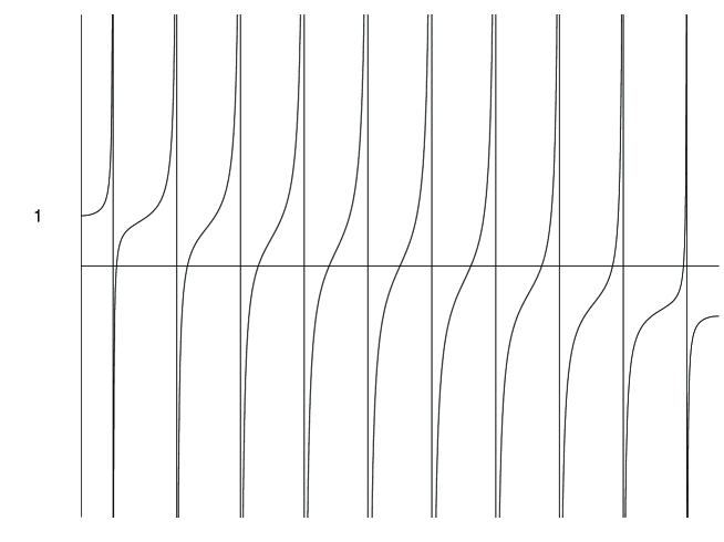
Figure 2: $k$ : even ,  $f_{k}(\rho)=\frac{\cos((N-2)\rho/2)}{\cos(N\rho/2)}\ ,\ 0\leq\rho\leq\pi,\$ with $N=20$

Hence the number of real solutions $\rho$ of (12) with $0<\rho<\pi$ is given by

$$\left\{\begin{array}[]{ll}\frac{N}{2}-2&\mbox{for \ odd \ }k\ \mbox{and \ }\ |\cos\frac{k\pi}{N}|<\frac{N-2}{N}\ ,\\ \frac{N}{2}-1&\mbox{for \ odd \ }k\ \mbox{and \ }|\cos\frac{k\pi}{N}|\geq\frac{N-2}{N}\ ,\\ \frac{N}{2}-1&\mbox{for \ even \ }k\ .\end{array}\right.$$

The total number is

$$\frac{N}{2}(N-3)+\#\{k=2j-1\ |\ 1\leq j\leq\frac{N}{2}\ ,\ |\cos\frac{k\pi}{N}|\geq\frac{N-2}{N}\}\ ,$$

and it is equal to the number of real solutions $\{\lambda_{1},\lambda_{2}\}$ of BAE for $l=2$, including those with the value $\infty$, which is the solutions corresponding to $\rho=\frac{k\pi}{N}$ for the equation (12). Hence the number of finite real Bethe solutions $\{\lambda_{1},\lambda_{2}\}$ for $l=2$ is equal to

$$\frac{N}{2}(N-3)-(N-1)+\#\{k=2j-1\ |\ 1\leq j\leq\frac{N}{2}\ ,\ |\cos\frac{k\pi}{N}|\geq\frac{N-2}{N}\}\ .$$ (13)

Since the total number of complex solutions of (12) is $N$, one obtains the contribution of non-real Bethe solutions for $l=2$ whose number is given by

$$\left\{\begin{array}[]{ll}1&\mbox{for \ odd \ }k\ \ \ \mbox{and \ }|\cos\frac{k\pi}{N}|<\frac{N-2}{N}\ ,\\ 0&\mbox{for \ odd \ }k\ \ \ \mbox{and \ }|\cos\frac{k\pi}{N}|\geq\frac{N-2}{N}\ ,\\ 1&\mbox{for \ even \ }k\ \ \ \mbox{and \ }k\neq 0\ ,\\ 0&\mbox{for \ }k=0\ ,\end{array}\right.$$

with the total number

$$N-1-\#\{k=2j-1\ |\ 1\leq j\leq\frac{N}{2}\ ,\ |\cos\frac{k\pi}{N}|\geq\frac{N-2}{N}\}\ .$$ (14)

Therefore the number of Bethe solutions for $l=2$ is the sum of (13) and (14), which is equal to $C^{N}_{2}-C^{N}_{1}$. This coincides with the counting of Bethe 2-states given in [9] . $\Box$

Example 3. Bethe solutions for $l=3\ ,N=6$. The BAE is given by

$$(\frac{\lambda_{j}+\frac{i}{2}}{\lambda_{j}-\frac{i}{2}})^{6}=-\prod_{m=1}^{3}\frac{\lambda_{j}-\lambda_{m}+i}{\lambda_{j}-\lambda_{m}-i}\ \ \ \ \ (j=1,2,3)\ \ ,\ \lambda_{j}\neq\lambda_{k}\in\,\hbox{IC}\ .$$

Claim: There are exactly 5 solutions of the above equation, and each of them is invaraint under the map $\lambda\rightarrow-\lambda$.

First let us consider a solution invariant under the sign symmetry: $\lambda\leftrightarrow-\lambda$. We may assume $\lambda_{j}$’s take the form

$$\lambda_{1}=-\lambda_{3}=\lambda\ \ (\neq 0)\ ,\ \ \ \lambda_{2}=0\ .$$

With the variable $z$ in (11), the corresponding equation of $z_{1}$ is

$$z^{6}-3z^{5}+3z-1=0\ .$$

The above equation has 6 distinct roots, which includes $z=1$. The value $\lambda$ corresponding to each of the other 5 solutions gives a Bethe solution symmetric under the change of sign. They contribute 5 independent states in the Hilbert space $\hbox{IH}_{6}$, which is a 64-dimensional vector space . On the other hand, by Example 1 and 2 of this section together with (iv) of Proposition 1, the total number of Bethe states $\Psi_{N}(\lambda_{1},\ldots,\lambda_{l})$ for $0\leq l\leq 2$ is equal to

$$1\times 7+5\times 5+9\times 3=59\ .$$

Therefore there is no other Bethe 3-state except the symmetric ones we have described. Then the conclusion follows immeadiately. $\Box$

Explicit Bethe solutions of a higher $l$ are difficult to obtain in general for a finite size $N$. For the rest of this paper, we shall consider only the case

$$l=g:=\frac{N}{2}\ \ {\rm and}\ \ \ \lambda_{j}\in\hbox{IR}\ \ \ {\rm for}\ \ j=1,\ldots,g\ .$$

The equation we are going to discuss is the following form:

$$(\frac{\lambda_{j}+\frac{i}{2}}{\lambda_{j}-\frac{i}{2}})^{N}=-\prod_{m=1}^{g}\frac{\lambda_{j}-\lambda_{m}+i}{\lambda_{j}-\lambda_{m}-i}\ \ ,\ \ \lambda_{j}\in\hbox{IR}\ \ (j=1,\ldots,g)\ .$$ (15)

The Bethe vector corresponding to the above Bethe roots leads to the ground state of antiferromagetic $H_{\rm XXX}$ (i.e. $J<0$ ) in $N\rightarrow\infty$. It is more convenient to consider the logarithmic form of the the above equation. By using the relation

$$\frac{1}{i}\log\frac{\lambda-i}{\lambda+i}=2\arctan(\lambda)+\pi\ ,\ \ \ \ |\arctan(\lambda)|<\frac{\pi}{2}\ \ \ \ \mbox{ for \ }\lambda\in\hbox{IR},$$

we obtain the following equation from (15):

$$\arctan 2\lambda_{j}=\pi\frac{Q_{j}}{N}+\frac{1}{N}\sum_{k=1}^{g}\arctan(\lambda_{j}-\lambda_{k})\ \ \ ,\ 1\leq j\leq g\ ,$$

where $Q_{j}$’s are all integers or all half-integers according to $g$ odd or even, and they are bounded by the number $\widetilde{Q}$ determined by the relation:

$$\arctan(\infty)=\frac{\pi}{N}(\widetilde{Q}+\frac{1}{2})+\frac{1}{N}\sum_{k=1}^{g}\arctan(\infty)\ .$$

Hence

$$\begin{array}[]{rl}\widetilde{Q}&=\frac{N}{4}-\frac{1}{2}\\ q_{j}:=\frac{Q_{j}}{N}&=\frac{-1}{4}-\frac{1}{2N}+\frac{j}{N}\ ,\ \ \ \ j=1,2,\dots,g,\end{array}$$

and (15) is now equivalent to the equation

$$\begin{array}[]{c}F_{j}(\Lambda):=\arctan 2\lambda_{j}-(\pi q_{j}+\frac{1}{N}\sum_{k=1}^{g}\arctan(\lambda_{j}-\lambda_{k}))=0\\[5.69054pt] \Lambda:=\left(\begin{array}[]{c}\lambda_{1}\\ \vdots\\ \lambda_{g}\end{array}\right)\in\hbox{IR}^{g}\ ,\ \ j=1,2,\dots,g.\end{array}$$ (16)

Since only a finite number of solutions can be obtained for BAE (15) by Propostion 1, we obtain the following result.

Lemma 2 . BAE (15) is equivalent to the equation (16) , which has at most a finite number of solutions. $\Box$

Now we are going to show the existence of real solutions for (16). Define the endomorphism $F$ and the linear involution $E$ of $\hbox{IR}^{g}$ by

$$\begin{array}[]{l}F:\hbox{IR}^{g}\longrightarrow\hbox{IR}^{g}\ ,\ \ F(\Lambda):=\left(\begin{array}[]{c}F_{1}(\Lambda)\\ \vdots\\ F_{g}(\Lambda)\end{array}\right)\\ E:\hbox{IR}^{g}\longrightarrow\hbox{IR}^{g}\ ,\ \ E(\Lambda)=\left(\begin{array}[]{c}\vdots\\ E(\Lambda)_{j}\\ \vdots\end{array}\right)\ ,\ \ E(\Lambda)_{j}:=-\lambda_{g+1-j}\ .\end{array}$$

Denote the $E$-invariant vector in $\hbox{IR}^{g}$:

$$q=\left(\begin{array}[]{c}q_{1}\\ \vdots\\ q_{g}\end{array}\right).$$

It is easy to see that $F$ has the following symmetry properties:

Lemma 3.

(i)

$$F(-\Lambda)=-F(\Lambda)-2\pi q\ \ \ \ {\rm for\ }\ \Lambda\in\hbox{IR}^{g}\ .$$

(ii) $F\circ E=E\circ F$. $\Box$

We are going to show the existence of solutions of the equation (16) by the fixed point theory.

Proposition 3 . For a sufficient large cube $C$ in $\hbox{IR}^{g}$

$$C=\{\Lambda=(\lambda_{1},\ldots,\lambda_{g})^{t}\in\hbox{IR}^{g}:-a\leq x_{j}\leq a,\ \ 1\leq j\leq g\ \}$$

there exists a solution for the equation $F(\Lambda)=\vec{0}$ in $\Lambda\in C$.

Proof. Since

$$\lim_{x\rightarrow\infty}(\arctan 2x-\frac{\pi}{4})=\frac{\pi}{4}$$

there is a positive number $\alpha$ such that

$$\arctan 2\alpha-\pi q_{g}=\arctan 2\alpha-\frac{\pi}{4}+\frac{\pi}{2N}>\frac{\pi}{4}\ .$$

Let $C$ be the cube in $\hbox{IR}^{g}$ with

$$a\geq\alpha\ \ .$$

Denote $C_{j}^{+},C_{j}^{-}$ the faces of $C$ :

$$C_{j}^{+}=\{\Lambda\in C\ |\ \lambda_{j}=a\}\ \ ,\ \ \ C_{j}^{-}=\{\Lambda\in C\ |\ \lambda_{j}=-a\}\ \ ,\ \ \ j=1,\ldots,g\ .$$

By the inequalities

$$\arctan 2a-\pi q_{j}\geq\arctan 2\alpha-\pi q_{g}>\frac{\pi}{4}\ \ ,\ \ \ \ \frac{1}{N}\sum_{k=1}^{g}\arctan(a-\lambda_{k}))\leq\frac{g\pi}{2N}=\frac{\pi}{4}$$

one has

$$F_{j}(\Lambda)>0\ \ {\rm for}\ \ \ \ \Lambda\in C_{j}^{+}\ .$$

For $\Lambda\in C_{j}^{-}$ and $j>[\frac{N}{4}]$, we have

$$q_{j}\geq 0\ ,\ \ -\Lambda\in C_{j}^{+}$$

hence by (i) of Lemma 3,

$$F_{j}(\Lambda)=-F_{j}(-\Lambda)-2\pi q_{j}<0\ .$$

For $\Lambda\in C_{j}^{-}$ and $j\leq[\frac{N}{4}]$, we have

$$E(\Lambda)\in C_{g+1-j}^{+}\ ,\ \ F_{g+1-j}(E(\Lambda))>0$$

hence by (ii) of Lemma 3,

$$F_{j}(\Lambda)=-F_{g+1-j}(E(\Lambda))<0\ .$$

Therefore we obtain

$$F_{j}(\Lambda)<0\ \ \ \ \ {\rm for}\ \Lambda\in C_{j}^{-}\ .$$

Thus by Poincaré-Miranda fixed point theorem, (see e.g. [2] p.p.12), the conclusion of the proposition follows immediately. $\Box$

Remark. (i) One can require the symmetry property on the solutions in the above proposition. Indeed there is a solution of $F(\Lambda)=0$ in the intersect of cube $C$ with the hypersurface $H$,

$$H:=\{\Lambda\in\,\hbox{IC}^{g}\ |\ E(\Lambda)=\Lambda\}\ .$$

In fact, the map $F$ sends $H$ into itself. Since $\lambda_{j},1\leq j\leq[\frac{N}{4}],$ form a coordinate system of $H$, the conclusion in the above proof implies that the map

$$F_{\rm rest}:H\cap C\longrightarrow H$$

also satisfies the the conditions of Poincaré-Miranda fixed point theorem, hence it follows the result.

(ii) The argument given in the proposition also provides an appriori estimate on the location of roots of $F(\Lambda)=\vec{0}$, which lies in the following region

$$\{\Lambda\ |\ b_{j}\leq\lambda_{j}\leq a_{j}\ ,\ 1\leq j\leq g\ \}$$

where

$$a_{j}=\frac{1}{2}\tan(\frac{\pi}{4}+\pi q_{j})\ \ \ \ \ b_{j}=\frac{1}{2}\tan(\frac{-\pi}{4}+\pi q_{j})\ \ .$$

$\Box$

As a corollary of Proposition 3 and Lemma 2 , we have the following result:

Proposition 4 . There is a solution of the equation (15). $\Box$

The uniqueness for the solution of (15) should be expected by the thermodynamic nature of the solutions. Let us look a few cases of small $N$. Note that if $\{\lambda_{j}\}_{j=1}^{g}$ satisfies the equation (16), they satisfy the following equality:

$$\sum_{j=1}^{g}\arctan(2\lambda_{j})=0\ .$$

For $N=4$, the above symmetry relation enables one to obtain the solution of the equation (16) which is equivalent to

$$\left\{\begin{array}[]{l}\lambda_{1}+\lambda_{2}=0\\ \arctan(2\lambda_{1})=\frac{-\pi}{8}+\frac{1}{4}\arctan(\lambda_{1}-\lambda_{2})\end{array}\right.$$

Hence

$$\lambda_{1}=\frac{-1}{2\sqrt{3}}\ ,\ \ \ \lambda_{2}=\frac{1}{2\sqrt{3}}\ .$$

For a general $N$, one can conclude that all the $\lambda_{j}$’s can not be of the same sign. Indeed one can determine signs of $\lambda_{1}$ and $\lambda_{g}$ from the first and the last relations in (16):

$$\arctan(2\lambda_{1})<\pi(\frac{-1}{4}+\frac{1}{2N})+(\frac{N}{2}-1)\frac{\pi}{2N}=0\ ,\ \ \arctan(2\lambda_{g})>\pi(\frac{1}{4}-\frac{1}{2N})-(\frac{N}{2}-1)\frac{\pi}{2N}=0$$

hence

$$\lambda_{1}<0<\lambda_{g}\ .$$ (17)

It appears to be the case that certain symmetry properties exist among $\lambda_{j}$’s, e.g.

$$\lambda_{1}<\lambda_{2}<\cdots<\lambda_{g}\ \ ,\ \ \ \ \ \ \lambda_{j}+\lambda_{g+1-j}=0\ ,$$

but the mathematical derivation from the equation (16) seems a difficult problem, even in the case of $N=6$:

$$\left\{\begin{array}[]{lll}\arctan(2\lambda_{1})&=&\frac{-\pi}{6}+\frac{1}{6}(\arctan(\lambda_{1}-\lambda_{2})+\arctan(\lambda_{1}-\lambda_{3}))\\ \arctan(2\lambda_{2})&=&\frac{1}{6}(\arctan(\lambda_{2}-\lambda_{1})+\arctan(\lambda_{2}-\lambda_{3}))\\ \arctan(2\lambda_{3})&=&\frac{\pi}{6}+\frac{1}{6}(\arctan(\lambda_{3}-\lambda_{1})+\arctan(\lambda_{3}-\lambda_{2}))\end{array}\right.$$ (18)

However in the above case, by the analysis of Example 3 in this section, the symmetry property for the solutions holds:

$$\lambda_{1}+\lambda_{3}=0\ \ ,\ \ \ \lambda_{2}=0\ .$$

Hence $\lambda_{1}$ satisfies the equation

$$5\arctan(2\lambda)-\arctan(\lambda)=\pi\ .$$

Since the left hand side is a strictly inceasing function of $\lambda$, there exists an unique solution of $\lambda_{1}$, hence the uniqueness of the equation (18). For a larger size $N$, the mathematical structure of the equation (16) becomes more complicated that no effective mean could be found at this moment for the uniqueness problem. In the next section, we shall present an plausible, but not a mathematically rigorous, argument on the unique ground state solution for a large but finite $N$ based on the thermodynamic limit procedure.

5 Ground State for Antiferromagnetic XXX Model

The ground state of the Hamiltonian $H_{\mbox{XXX}}$ for the antiferromagnetic case is the state for the solution of (16). In the thermodynamic limit, one assumes there is a real solution $\{\lambda_{j}\}_{j=1}^{\frac{N}{2}}$ for the asymtotic equation of (16):

$$\arctan 2\lambda_{j}\sim\pi q_{j}+\frac{1}{N}\sum_{k=1}^{\frac{N}{2}}\arctan(\lambda_{j}-\lambda_{k})\ ,\ \ 1\leq j\leq\frac{N}{2}\ .$$

The $q_{j}$’s are considered as quantum numbers of the ground state. As $N$ tends to $\infty$, the continuous version of the above relation is obtained by the following substitution :

$$q_{j}\longrightarrow x\in(\frac{-1}{4},\frac{1}{4})\ \ ,\ \ \ \ \lambda_{j}\longrightarrow\lambda(x)\ \ ,$$

here $\lambda(x)$ is a monotonic increasing function with $\lambda(\frac{-1}{4})=-\infty$ and $\lambda(\frac{1}{4})=\infty$. The density of the ground state is now defined to be

$$\rho_{v}(\lambda)=\frac{dx}{d\lambda}\ \ \ (\ =\lim_{N\rightarrow\infty,\lambda_{j}\rightarrow\lambda}\frac{1}{N(\lambda_{j+1}-\lambda_{j})}\ ).$$

The logarithmic BAE for the ground state now becomes

$$\arctan 2\lambda(x)=\pi x+\int_{-\frac{1}{4}}^{\frac{1}{4}}\arctan(\lambda(x)-\lambda(y))dy.$$

Differentiating the above equation with respect to $x$, one can derive the integral equation for $\rho_{v}$:

$$\pi\rho_{v}(\lambda)+(\frac{1}{1+\mu^{2}}\ast\rho_{v})(\lambda)=\frac{2}{1+4\lambda^{2}}\$$ (19)

here the convolution of function $f$ and $g$ is defined by

$$(f\ast g)(\lambda)=\int_{-\infty}^{\infty}f(\lambda-\mu)g(\mu)d\mu.$$

Then the density, energy , momentum and spin of the ground state in the thermodynamic limit for the antiferromagnetic XXX model are given by

$$\rho_{v}(\lambda)=\frac{1}{2\cosh(\pi\lambda)},\ \ E_{v}=JN\log 2\ ,\ \ \Pi_{v}=\frac{N\pi}{2}\ \ (\mbox{mod \ }2\pi),\ \ S_{v}=0\ .$$

( For the details, see [5] [10] ).

Now we explain the reason for the uniqueness of the ground state for a large but finite $N$. Suppose that $\{\lambda_{j}\}_{j=1}^{N/2}$ is a set of solutions of (16) such that the density $\rho_{v}(\lambda)$ of the continuous limit $\lambda(x)$ is given by $\frac{1}{2\cosh(\pi\lambda)}$. Without loss of generality, we may assume there is another set of real solutions $\{\widetilde{\lambda}_{j}\}_{j=1}^{l}$ of the equation (16) for a size $N$. Then for some $\mu_{j}$, one has the expansion:

$$\widetilde{\lambda}_{j}=\lambda_{j}+\frac{1}{N}\mu_{j}+O(\frac{1}{N^{2}})\ \ \ \ \ ,\ j=1,\ldots,\frac{N}{2}\ .$$

We have

$$\arctan(2\lambda_{j})+\frac{2\mu_{j}}{N(1+4\lambda_{j}^{2})}=\pi q_{j}+\frac{1}{N}\sum_{k=1}^{N/2}[\arctan(\lambda_{j}-\lambda_{k})+\frac{1}{1+(\lambda_{j}-\lambda_{k})^{2}}\frac{\mu_{j}-\mu_{k}}{N}]+O(\frac{1}{N^{2}})\ ,$$

hence

$$\frac{2\mu_{j}}{N(1+4\lambda_{j}^{2})}=\frac{1}{N}\sum_{k=1}^{N/2}[\arctan(\lambda_{j}-\lambda_{k})+\frac{1}{1+(\lambda_{j}-\lambda_{k})^{2}}\frac{\mu_{j}-\mu_{k}}{N}]+O(\frac{1}{N^{2}})\ .$$

In the continuous limit,

$$\lambda_{j}\longrightarrow\lambda(x)\ ,\ \ \mu_{j}\longrightarrow\mu(x)\ \ \ \ {\rm for}\ \ x\in(\frac{-1}{4},\frac{1}{4})\ ,$$

the above equation becomes

$$\frac{2\mu(x)}{1+4\lambda(x)^{2}}=\int_{\frac{-1}{4}}^{\frac{1}{4}}\frac{\mu(x)-\mu(y)}{1+(\lambda(x)-\lambda(y))^{2}}dy\ .$$

Therefore

$$\frac{2\mu(\lambda)}{1+4\lambda^{2}}=\int_{-\infty}^{\infty}\frac{\mu(\lambda)-\mu(\nu)}{1+(\lambda-\nu)^{2}}\rho_{v}(\nu)d\nu\$$

and

$$\mu(\lambda)[\frac{2\mu(\lambda)}{1+4\lambda^{2}}-\int_{-\infty}^{\infty}\frac{\rho_{v}(\nu)}{1+(\lambda-\nu)^{2}}d\nu]=-\int_{-\infty}^{\infty}\frac{\mu(\nu)\rho_{v}(\nu)}{1+(\lambda-\nu)^{2}}d\nu.$$

By (19), one has

$$\pi\mu(\lambda)\rho_{v}(\lambda)=-\int_{-\infty}^{\infty}\frac{\mu(\nu)\rho_{v}(\nu)}{1+(\lambda-\nu)^{2}}d\nu\ \ .$$

By taking Fourier transform, the above equation becomes

$$\pi\widehat{\mu\rho_{v}}=\widehat{\frac{-1}{1+\lambda^{2}}}\widehat{\mu\rho_{v}}$$

which implies $\mu(x)=0$. Therefore $\lambda_{j}$ and $\widetilde{\lambda}_{j}$ agree up to the order of $\frac{1}{N^{2}}$. Repeating the same procedure inductively to higher order terms of $\frac{1}{N}$, one arrives the conclusion that $\lambda_{j}$ coincides with $\widetilde{\lambda}_{j}$ for all $j$.

References

[1] R. J. Baxter, Exactly solved models in statistical mechanics,
Academic Press (1982).
[2] F. E. Browder, Fixed point theory and
non-linear problems, Bull. AMS 9 (1983) 1-39.
[3] F. H. L. Essler, V. E. Korepin and K. Schoutens,
Fine structur of the Bethe ansatz for the spin- Heisenberg
XXX model, J. Phys. A: Math. Gen. 25 (1992) 4115-4126.
[4] L. D. Faddeev, Algebraic aspects of Bethe-Ansatz, ITP-SB-94-11,
[5] L. D. Faddeev and L. A. Takhtadzhan , Spectrum
and scattering of excitations in the one-dimensional
isotropic Heisenberg model, J. Soviet Math. 24 (1984) 241-267.
[6] A. G. Izegin and V. E. Korepin, Pauli principal
for one-dimensional bosons and the algebraic Bethe Ansatz,
Lett. Math. Phy. 6 (1982) 283-288.
[8] L. A. Takhtadzhan and L. D. Faddeev , The quantum method
of the inverse problem and the Heisenberg XYZ model, Russian Math. Surveys
34: 5 ( 1979 ), 11 - 68.
[9] L. A. Takhtadzhan and L. D. Faddeev , What is
the spin of a spin wave, Phys. Letts 85A, No 6,7 (1981)
375 - 377.
[10] C. N. Yang and C. P. Yang, One dimensional chain
of anisotropic spin-spin interaction. I. Proof of Bethe’s
hypothesisfor ground state in finite system, Phy. Rev. 150
(1966) 321-327 , II. Properties of ground state energy per
lattice site for a finite system, Phy. Rev. 150 (1966)
327-339.