Transfer of Spectral Weight in Spectroscopies of Correlated Electron Systems

Abstract

We study the transfer of spectral weight in the photoemission and optical spectra of strongly correlated electron systems. Within the LISA, that becomes exact in the limit of large lattice coordination, we consider and compare two models of correlated electrons, the Hubbard model and the periodic Anderson model. The results are discussed in regard of recent experiments. In the Hubbard model, we predict an anomalous enhancement optical spectral weight as a function of temperature in the correlated metallic state which is in qualitative agreement with optical measurements in $V_{2}O_{3}$. We argue that anomalies observed in the spectroscopy of the metal are connected to the proximity to a crossover region in the phase diagram of the model. In the insulating phase, we obtain an excellent agreement with the experimental data and present a detailed discussion on the role of magnetic frustration by studying the $k-$resolved single particle spectra. The results for the periodic Anderson model are discussed in connection to recent experimental data of the Kondo insulators $Ce_{3}Bi_{4}Pt_{3}$ and $FeSi$. The model can successfully explain the different energy scales that are associated to the thermal filling of the optical gap, which we also relate to corresponding changes in the density of states. The temperature dependence of the optical sum rule is obtained and its relevance for the interpretation of the experimental data discussed. Finally, we argue that the large scattering rate measured in Kondo insulators cannot be described by the periodic Anderson model.

I Introduction.

The interest in the distribution of spectral weight in the optical conductivity of correlated electron systems has been revived by the improvement of the quality of the experimental data in various systems [1, 2, 3].

The traditional methods used in the strong correlation problem, exact diagonalization of small clusters [4], slave boson approaches[5], and perturbative calculations, have not been very successful in describing the interesting transfer of optical weight which takes place as a function of temperature in the strong correlation regime.

Recently, much progress has been achieved by mapping lattice models into impurity models embedded in an effective medium. This technique, the Local Impurity Selfconsistent Approximation (LISA) [6], is a dynamical mean field theory that becomes exact in the limit of large number of spatial dimensions [7]. For instance, the Hubbard and the Anderson lattice model can be mapped onto the Anderson impurity model subject to different selfconsistency conditions for the conduction electron bath [8, 9]. These resulting selfconsistent impurity problems can be analyzed by a variety of numerical techniques [10, 11, 12, 13, 14, 15, 16, 17, 18, 19].

In this paper we apply this approach to the study of the optical conductivity in regard of the recent experiments in $V_{2}O_{3}$, $Ce_{3}Bi_{4}Pt_{3}$, and $FeSi$. We take the view that the low energy optical properties of $V_{2}O_{3}$ can be modeled by a one band Hubbard model, while $Ce_{3}Bi_{4}Pt_{3}$ and $FeSi$ are described by a periodic Anderson model [20]. The modeling of the experimental systems requires a large value of the Coulomb repulsion $U$.

Our main goal in this work is to demonstrate that simplified models of strongly interacting systems treated with the LISA, can account for the main qualitative features that are observed experimentally in strongly correlated electron compounds. The paper is organized as follows: in section II we summarize the mean field equations for the model hamiltonians and the expressions for the calculation of the optical conductivity and the optical sum rule. In section III we present and intuitive pedagogical discussion the physical content of the solution of the model hamiltonians in the large dimensional limit. Section IV is dedicated to a thorough discussion of the optical conductivity results. We discuss the effects of magnetic frustration on the spectral functions of the Hubbard model. And the effects of temperature and disorder on the optical spectra of the Anderson lattice. The theoretical calculations are carried out using exact diagonalization (ED) and iterated perturbation theory (IPT) techniques, and compared with texperimental results on various systems. We stress that the use of IPT allow us to access physically interesting regimes which are outside the scope of the Quantum Monte Carlo method, and that the exact diagonalization technique is used to confirm that the results presented are genuine features of the Hubbard model in infinite dimensions and not artifacts of the IPT. The conclusions are presented in the last section. Our ED approach to the solution of correlated models in large dimensions is based on the use continuous fractions. The Appendix describes an algorithm to convert the sum of two given continued fractions into a new continued fraction which we use to extend the ED method to the models we treat in this paper. Part of the theoretical results in section IV were announced in a recent letter [21] . The optical conductivity of the Anderson model and the Hubbard model were considered previously by Jarrell et al. using the Qauntum Monte Carlo and Maximum Entropy methods. [14, 22, 23]

II Methodology.

A Mean field equations.

As model hamiltonians we consider the Hubbard and the periodic Anderson model (PAM):

$$H_{H}=-\sum_{<i,j>}(t_{ij}+\mu)c_{i\sigma}^{\dagger}c_{j\sigma}+\sum_{i}U(n_{i\uparrow}-\frac{1}{2})(n_{i\downarrow}-\frac{1}{2}),$$ (1)

$$H_{PA} = \sum_{k}(\epsilon_{k}-\mu)c_{k\sigma}^{\dagger}c_{k\sigma}+\sum_{i}({\epsilon}^{o}_{d}-\mu)d_{i\sigma}^{\dagger}d_{i\sigma}$$ (2)

$$+ \sum_{i}Vd^{\dagger}_{i\sigma}c_{i\sigma}+h.c.+\sum_{i}U(n_{di\uparrow}-\frac{1}{2})(n_{di\downarrow}-\frac{1}{2})$$ (3)

where summation over repeated spin indices is assumed. $\mu$ is the chemical potential, and $t_{ij}$ is the hopping amplitude between the conduction electron sites, which in the PAM results in the band $\epsilon_{k}$. The $d^{\dagger}$ and $d$ operators create and destroy electrons on localized orbital with energy $\epsilon_{d}^{o}$. $V$ is the hybridization amplitude between $c$ and $d-$sites, which also appear in the literature as $d$ and $f-$sites respectively.

The derivation has been given in detail elsewhere [8, 9]. So we only present the final expressions. The resulting local effective action reads,

$${S}_{local} = -\int^{\beta}_{0}d\tau\int^{\beta}_{0}d\tau^{\prime}\psi^{\dagger}_{\sigma}(\tau){\cal G}_{0}^{-1}(\tau-\tau^{\prime})\psi_{\sigma}(\tau^{\prime})$$ (4)

$$+ \ U\ \int^{\beta}_{0}d\tau(n_{\uparrow}(\tau)-{1\over 2})(n_{\downarrow}(\tau)-{1\over 2})$$ (5)

where $\psi^{\dagger}_{\sigma},\ \psi_{\sigma}$ correspond to a particular site, and denote $c^{\dagger}_{\sigma},\ c_{\sigma}$ in the Hubbard model, and $\{c^{\dagger}_{\sigma},d_{\sigma}^{\dagger}\},\ \{c_{\sigma},d_{\sigma}\}$ in the PAM case. $n_{\sigma}$ corresponds to $n_{c\sigma}$ and $n_{d\sigma}$ respectively. Also note that Eq.5 defines the associated impurity problem, with $\psi^{\dagger}_{\sigma},\ \psi_{\sigma}$ being the operators at the impurity site while the information on the hybridization with the environment is implicitly contained in ${\cal G}_{0}^{-1}$. Requiring that $G_{local}(\omega)=\Sigma_{k}G(k,\omega)$, we obtain as selfconsistency condition

$${\cal G}_{0}^{-1}(\omega)=\omega+\mu-t^{2}\tilde{G}(\omega)$$ (6)

for the Hubbard model, and

$$[{\cal G}_{0}^{-1}]_{cc}(\omega)=\omega+\mu-t^{2}[\tilde{G}]_{cc}(\omega)$$ (7)

with ${\cal G}_{0}$ explicitly given by

$${\cal G}_{0}^{-1}(i\omega)=\left(\begin{array}[]{cc}i\omega-{t^{2}}[\tilde{G}]_{cc}(i\omega)&V\\ V&i\omega\end{array}\right)$$ (8)

for the PAM. In both cases, $\tilde{G}$ is the “cavity” Green function which has the information of the response of the lattice.

We will consider the symmetric case with $\mu=0$ and $\epsilon^{o}_{d}=0$. Moreover, we assume a semi-circular bare density of states for the conduction electrons, $\rho^{o}(\epsilon)=\sum_{k}\delta(\epsilon-\epsilon_{k})/N_{sites}=(2/{\pi D})\sqrt{1-(\epsilon/D)^{2}}$, with the half-bandwidth $D=2t$. This density of states can be realized in a Bethe lattice and also on a fully connected fully frustrated version of the model [13, 15]. In this case the “cavity” Green function simply becomes $\tilde{G}=G$. In the following we set the half-bandwidth $D=1$. We use an exact diagonalization algorithm (ED) [17, 18] and an extension of the second order iterative perturbation theory (IPT) to solve the associated impurity problem [13]. We have checked that IPT and the ED method are in good agreement for all values of the model parameters. This results from the property of IPT to capture the atomic limit exactly in the symmetric case[13]. We use extensively the IPT on the real axis to scan through parameter space. A detailed comparison will be presented elsewhere.

B Optical conductivity.

The optical conductivity of a given system is defined by

$$\sigma(\omega)={1\over{\cal V}\,\omega}\mbox{Im}\,\int_{0}^{\infty}\langle[{\cal J}(t),{\cal J}(0)]\rangle e^{i\omega t}dt$$ (9)

where ${\cal V}$ is the volume, ${\cal J}$ is the current operator and $\langle$ $\rangle$ indicates an average over a finite temperature ensamble or over the ground state at zero temperature. In general $\sigma(\omega)$ obeys a version of the f-sum rule [24, 25],

$$\int_{0}^{\infty}\sigma(\omega)d\omega={\pi\over{\cal V}}{\rm Im}\langle[P,{\cal J}]\rangle$$ (10)

where $P$ is a polarization operator obeying $\frac{\partial P}{\partial t}={\cal J}$.

In a model which includes all electrons and all bands the current operator ${\cal J}$ is given by

$${\cal J}=\frac{e}{m}\sum_{i}p_{i}\delta(r-r_{i})$$ (11)

where $p_{i}$ is the momentum and $r_{i}$ the position of the ${\rm i}^{th}$-electron, and $e$ and $m$ denote its charge and bare mass. $P$ is given by

$$P=e\sum_{i}r_{i}\delta(r-r_{i}).$$ (12)

Thus, ${1\over{\cal V}}\langle[P,{\cal J}]\rangle=\frac{ine^{2}}{m}$ where $n$ is the density of electrons, and the sum rule becomes

$$\int_{0}^{\infty}\sigma(\omega)d\omega=\pi\frac{ne^{2}}{m}.$$ (13)

This result is clearly temperature independent and does not depend either on the strength of the interactions.

When dealing with strongly correlated electron systems, in a frequency range where few of the bands are believed to be important, it is customary to work with an effective model with one or two bands, such as the Hubbard or the periodic Anderson model. The current operator is thus projected onto the low energy sector and is expressed in terms of creation and destruction operators of the relevant bands (i.e., ${\cal J}=i\frac{t}{\cal V}\sum_{i}(c^{\dagger}_{i+\delta}c_{i}-c_{i}^{\dagger}c_{i+\delta})$ for the Hubbard and Anderson model). It is in this case that the expectation value $\langle[P,{\cal J}]\rangle$ is no longer $\sim\frac{ne^{2}}{m}$, but, proportional to the expectation value of the kinetic energy $\langle K\rangle$ of the conduction electrons[24, 26]. In general $\langle K\rangle$ depends on the temperature and strength of interactions, therefore, for these few bands models, the optical weight sum rule will depend on them as well. If the projection onto a few band model is valid, this result also implicitly indicates that a portion of the optical spectral weight (the weight not exhausted by $\langle K\rangle$) is transferred to much higher energies, that is, to the bands that were excluded by the projection to low energies.

In this paper we do not address the question of the validity of the low energy projection onto a few band model. Instead we focus on the consequences of this assumption on the redistribution of the optical weight within a mean field theory that is exact in the limit of large dimensions. Our main conclusion is that there is a considerable temperature dependence of the integrated spectral weight appearing in the sum rule.

In infinite dimensions, $\sigma(\omega)$ can be expressed in terms of the one particle spectrum of the current carrying electrons [27, 23]:

$$\sigma(\omega) = \frac{1}{\omega}\frac{2e^{2}t^{2}a^{2}}{\nu\hbar^{2}}\int_{-\infty}^{\infty}{d\epsilon}\ {\rho^{o}(\epsilon)}\int_{-\infty}^{\infty}\frac{d\omega^{\prime}}{2\pi}$$ (15)

$$A_{\epsilon}(\omega^{\prime})A_{\epsilon}(\omega^{\prime}+\omega)(n_{f}(\omega^{\prime})-n_{f}(\omega^{\prime}+\omega))$$

with $A_{\epsilon}(\omega)=-2{\rm Im}[G_{k}(\omega)]$ being the spectral representation of the Green function of the lattice conduction electrons, $a$ the lattice constant, and $\nu$ the volume of the unit cell.

As we anticipated, the kinetic energy is related to the conductivity by the sum rule

$$\int_{0}^{\infty}\sigma(\omega)d\omega=-\frac{\pi e^{2}a^{2}}{2d\hbar^{2}\nu}\langle K\rangle=\frac{\omega_{P}^{2}}{4\pi}$$ (16)

An important result, which will be demonstrated later on, is the notable dependence of the plasma frequency $\omega_{P}$ with temperature. This feature will be seen to emerge as consequence that correlation effects generate small energy scales (e.g. the “Kondo temperature” of the associated impurity). It is the competition between the small scales and the temperature that gives rise to an unusual temperature dependence to the integrated optical spectral weight.

At $T=0$, the optical conductivity of a metallic correlated electron system can be parametrized by [25]

$$\sigma(\omega)=\frac{{\omega^{*}_{P}}^{2}}{4\pi}\delta(\omega)+\sigma_{reg}(\omega)$$ (17)

where the coefficient in front of the $\delta$-function is the Drude weight and $\omega^{*}_{P}$ is the renormalized plasma frequency. In the presence of disorder $\delta(\omega)$ is replaced by a lorentzian of width $\Gamma$.

Evaluating equation (15) at $T=0$ one finds in mean field theory that,

$$\frac{{\omega^{*}_{P}}^{2}}{4\pi}=\frac{2\pi e^{2}}{\hbar^{2}\nu}Z\sum_{k}\big{(}\frac{\partial\epsilon_{k}}{\partial k_{x}}\big{)}^{2}\delta(\epsilon_{k})$$ (18)

where $Z$ is the quasiparticle weight. For the Hubbard model in infinite dimensions the expression above further simplifies, and it only depends on the density of states

$$\frac{{\omega^{*}_{P}}^{2}}{4\pi}=\frac{4\pi t^{2}e^{2}a^{2}}{\hbar^{2}\nu}Z\rho^{o}(0).$$ (19)

III Physical Content of the Mean Field Theory.

A Hubbard Model.

The solution of the mean field equations shows that at low temperatures the model has a metal insulator transition (Mott-Hubbard transition) at an intermediate value of the interaction $U_{c}\approx 3D$ [14, 15, 16]. The metallic side is characterized by a density of states with a three peak structure: a central feature at the Fermi energy that narrows as one moves towards $U_{c}$ from below, and two broader incoherent features that develop at $\pm\frac{U}{2}$, namely, the lower and upper Hubbard bands. They have a width $\approx 2D$ and their spectral weight increases as the transition is approached. The insulator side, for $U>U_{c}$, presents only these last two high frequency features, which are separated by an excitation gap of size $\Delta\approx U-2D$. The different structures of the DOS (Fig.1) give rise to very different optical responses.

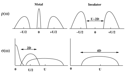
FIG. 1.: Schematic DOS for the Hubbard model (1/2 filling) and their corresponding optical spectra for the metallic and insulator solutions. The width of the incoherent peaks in the $DOS$ is $\approx 2D$ and the one of central peak in the metal is $\approx ZD\equiv\epsilon_{F}^{*}$.

Lets first consider the insulator, which is simpler. In this case, optical transitions are possible from the lower to the upper Hubbard band. We therefore expect the optical spectrum that results from the convolution (15) to display a single broad feature that extends approximately from $U-2D$ to $U+2D$ (Fig.1). A negligible temperature dependence of the spectra is expected, as long as $T<<\Delta$. On the other hand, in the metallic case, the low temperature optical spectrum displays various contributions: i) A narrow low frequency peak that is due to transitions within the quasiparticle resonance, in the $T=0$ limit this peaks becomes a $\delta-$function and is the Drude part of the optical response. ii) At frequencies of order $U\over 2$ an incoherent feature of width $\sim 2D$ emerges due to transitions between the Hubbard bands and the central resonance. iii) A last contribution at frequency $\sim U$ appears due to transitions between the Hubbard bands. This is a broad feature of width $\sim 4D$. Therefore, we expect an optical spectrum which is schematically drawn in Fig.1. It is important to realize that, unlike the insulator, a notable temperature dependence of the spectra is to be expected. There is a low energy scale $T_{coh}$ that corresponds to the temperature below which coherent quasiparticle excitations are sustained. It roughly corresponds to the the width of the resonance at the Fermi energy $\epsilon^{*}_{F}\equiv ZD$. As $T$ is then increased and becomes comparable to $T_{coh}$, the quasiparticles are destroyed, and in consequence, the contributions to the optical spectra associated with them, $(i)$ and $(ii)$, rapidly decrease.

It should be clear that in our previous discussion we have assumed that the system does not order magnetically, as paramagnetic solutions were considered. This situation can in fact be realized by introduction of disorder (e.g. a random distribution of $t_{ij}$) or next nearest neighbor hopping, and avoids the artificial nesting property of the bipartite lattice [15, 16].

B Periodic Anderson Model.

We now present a schematic discussion of the periodic Anderson model solution. In this case there are two different types of electrons, the $c$-electrons which form a band and the $d$-electrons with localized orbitals. In the non-interacting particle-hole symmetric case, the hybridization amplitude $V$ opens a gap in the $c-$electron density of states $\Delta_{ind}\sim V^{2}/D$. On the other hand, the original $\delta-$function peak of the localized $d-$electrons broadens by hybridizing with the conduction electrons and also opens a gap $\Delta_{ind}$.

When the effect of the interaction term is considered, as the local repulsive $U$ is increased, one finds that for low frequencies the non-interacting picture which was just described still holds, however, with the bare hybridization $V$ being renormalized to a smaller value $V^{*}$. Thus, we say we have a hybridization band insulator with the hybridization amplitude renormalized by interactions. This can also be interpreted by considering that the interacting $d-$electrons form a band of “Kondo-like” quasiparticles, that allows to define a coherence temperature $T^{*}$ similar to the $T_{coh}$ introduced before. This coherent band further opens a gap due to the periodicity of the lattice. This is the well known scenario that is born out from slave boson mean field theory and variational calculations [28]. On the other hand, the present dynamical mean field theory also captures the high energy part of the $d-$electron density of states that develops incoherent satellite peaks at frequencies $\pm\frac{U}{2}$ with spectral weight that is transferred from low frequencies. Consequently, the $c-$electron density of states is mainly made of a central broad band of half-width $D=2t$ and a gap at the center that gets narrower as $V\rightarrow V^{*}$. Also, it develops some small high frequency structures, that result from the hybridization with the d-electrons. In Fig.2 we schematically present the density of states for the $c$ and $d-$electrons. As in the Hubbard model, we assume the absence of magnetic long range order (MLRO). For a study of the magnetic phase of the Anderson model see Ref.[29].

FIG. 2.: Schematic DOS (1/2 filling) for $c$ and $d-$electrons in the PAM (top). The corresponding schematic optical spectra at $T=0$ (bottom left) and the schematic band structure with the direct and indirect gaps (bottom right).

Since the $d-$sites are localized orbitals, only the $c-$electrons contribute to the optical response of this system. At $T=0$, following the previous interpretation in terms of a renormalized non-interacting hybridization band insulator and equation (15), we expect to find an optical conductivity spectra with a gap $\Delta_{dir}$, which decreases as the interaction is increased. We also expect that $\Delta_{ind}<<\Delta_{dir}$, as the first corresponds to the indirect gap from the density of states $\Delta_{ind}\sim{V^{*}}^{2}/D$, while the second is the direct gap $\Delta_{dir}\sim{V^{*}}$ that is defined as the minimum energy for interband transitions at a given $k$ (see Fig.2). We do not expect any other important contributions to the optical response since, as we argued before, the incoherent high frequency structures of the $c-$electron density of states do not carry much spectral weight. In Fig.2 we schematically present the optical response at $T=0$.

As the temperature is increased the gap in the optical conductivity becomes gradually filled. At high temperatures a simple picture of electrons scattering off local moments emerge. The crossover between these two regimes, would naively occur at a temperature of the order of $\Delta_{ind}$.

Thus, we note that in the Hubbard model and in the periodic Anderson model the destruction of a coherent quasiparticle state that sets the low energy scale of the system has rather opposite effects in the optical response. In the first case, the correlated metallic state is destroyed as $T$ becomes of the order of the renormalized Fermi energy, and the Drude part of the optical response is transferred to higher energies as the insulating state sets in. In the second case, however, the destruction of the coherent excitations is accompanied by the thermal closing of the gap in the density of states that turns the system metallic. As a consequence, the gap of the optical response is filled with spectral weight from higher energies to become a broad Drude-like feature.

IV Results

A Hubbard model.

We will discuss the results for the model in regard of different experimental data on the $V_{2}O_{3}$ system. Vanadium oxide has three $t_{2g}$ orbitals per $V$ atom which are filled with two electrons. Two electrons (one per $V$) are engaged in a strong cation-cation bond, leaving the remaining two in a twofold degenerate $e_{g}$ band [30]. LDA calculations give a bandwidth of $\sim 0.5eV$ [31]. The Hubbard model ignores the degeneracy of the band which is crucial in understanding the magnetic structure [30], but captures the interplay of the electron-electron interactions and the kinetic energy. This delicate interplay of itinerancy and localization is responsible for many of the anomalous properties of this compound, and it is correctly predicted by this simplified model.

Experimentally one can vary the parameters $U$ and $D$, by introducing $O$ and $V$ vacancies or by applying presure or chemical substitution of the cation. We can use experimental data to extract approximate parameters to be used as input to our model. In particular, from the experimental optical conductivity data in the insulating phase, a rather accurate determination can be made because, as it is apparent from the spectra, the low frequency contribution is mainly due to a single peak [1]. In regard of our schematic discussion of the previous section, the position of the maximum should approximately correspond to the parameter $U$ that corresponds to transitions from the lower to the upper Hubbard band. Also, according to the picture of the previous section, the total width of the peak should be $\sim 4D$ which is twice the width of the Hubbard bands. Therefore, we can approximately estimate the parameter $D$ as the distance from position of the peak maximum to the frequency where the feature decreased to half its height (see Fig.3).

FIG. 3.: The experimental $\sigma(\omega)$ of insulating $V_{2-y}O_{3}$ with $y=0.013$ at $10K$ (upper) and $y=0$ at $70K$ (lower). We indicate in the spectra the position of the maxima and their width from which the parameters $U$ and $D$ for the model calculations are extracted.

The parameters from the metallic optical conductivity spectra are not so easily extracted. However, we can still obtain a rather precise determination by considering the difference spectra between the data at $170K$ and at $300K$ (see inset of Fig.4).

FIG. 4.: The experimental $\sigma(\omega)$ of metallic $V_{2}O_{3}$ at $T=170K$ (upper) and $T=300K$ (lower). The inset contains the difference of the two spectra $\Delta\sigma(\omega)=\sigma_{170K}(\omega)-\sigma_{300K}(\omega)$. Diamonds indicate the measured dc conductivity $\sigma_{dc}$.

As we shall later discuss in detail, it turns out that the feature that appears in the difference spectra at a frequency $\approx 0.4eV$ can be associated with the parameter $U/2$. This is also intuitively suggested by the schematic discussion of the previous section, as this feature corresponds to the enhancement of transitions from the lower Hubbard band to the central resonance at the Fermi level and from the resonance to the upper Hubbard band which are at a distance $\sim U/2$. The value for the parameter $D\approx 0.4eV$ in the metallic phase was determined by noting that: i) a priori there is no reason to expect that it should be much different than in the insulating phase (unlike the parameter $U$ which could be modified by screening); ii) it is consistent with the recent LDA calculation that gives a half-width of $\approx 0.5eV$ for the narrow bands at the Fermi level [31]; iii) despite the lack of very good experimental resolution the value is consistent with both the optical data that we reproduce in Fig.4 and photoemission experiments [32]; iv) as will be shown later in the paper, this estimated value will allow to gather in a single semi-quantitative consistent picture the optical conductivity results with the $V_{2}O_{3}$ phase diagram and experimental results for the slope of the specific heat. The extracted parameters along with the values for the size of the optical gap (in the insulators) and the total optical spectral weight are summarized in table I.

Phase	Parameter
	D [eV]	U [eV]	$\Delta$ [eV]	$\omega_{P}^{2}/4\pi$ [eV/$\Omega$cm]
Ins. (y=0)	$.33\pm.05$	$1.3\pm.05$	$.64\pm.05$	$170\pm 20$
Ins. (y=.013)	$.46\pm.05$	$.98\pm.05$	$.08\pm.05$	$800\pm 50$
Metal (170K)	$.4\pm.1$	$.8\pm.1$	–	$1700\pm 300$

TABLE I.: Experimental parameters for the model.

In Fig.5 we display the phase diagram of the model in large dimensions generalized to include $n.n.$ hopping $t_{1}$ and $n.n.n.$ hopping $t_{2}$. The condition $t_{1}^{2}+t_{2}^{2}=t^{2}$ keeps the bare density of states $\rho^{0}$ invariant. For $t_{2}/t_{1}=0$ we recover the original hamiltonian, and $t_{2}/t_{1}=1$ gives the paramagnetic solution. The extra hopping provides a magnetically frustrating interaction [16]. This phase diagram obtained for $t_{2}/t_{1}=\sqrt{1/3}$ has the same topology as the experimental one [33, 34, 35]. Frustration lowers the $T_{Neel}$ well below the second order $T_{MIT}$ point [16]. Using the parameters of table I, $T_{MIT}\approx 240K$, which is only within less than a factor of 2 from the experimental result. The dotted line indicates a crossover separating a good metal at low $T$ and a semiconductor at higher $T$. Between these states $\rho_{dc}(T)$ has an anomalous rapid increase, as is shown in the results of Fig.6. The reason for this feature can be traced to the thermal destruction of the coherent central quasiparticle peak in the $DOS$. We find the behavior of $\rho_{dc}(T)$ to be in good agreement with the experimental results of Mc Whan et al. [34]. Another crossover is indicated by a shaded area, it separates a semiconducting region with a gap $\Delta$ comparable with $T$ from a good insulator where $T<<\Delta$, consequently the crossover temperature increases linearly with $U$ and the horizontal width of the crossover region becomes broader with increasing $T$. This crossover is characterized by a sudden increase in $\rho_{dc}$ as function of $U$ at a fix $T$ (inset Fig.5). This crossover behavior was experimentally observed in $V_{2}O_{3}$ by Kuwamoto et al. [33].

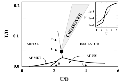
FIG. 5.: Approximate phase diagram for the model with $n.n.$ and $n.n.n.$ hopping $(t_{2}/t_{1})=\sqrt{1/3}$. The $1st$ order paramagnetic metal-insulator transition ends at the critical point $T_{MIT}$ (square). The dotted line and the shaded region describe two crossovers as discussed in the text. The full circles indicate the position of the optical spectra. $A$: insulator ($y=0$), $B$: insulator ($y=.013$), $C$: metal ($y=0,\ 170K$), $D$: metal ($y=0,\ 300K$). Note that for comparison with experimental results increasing $U/D$ is associated with decreasing pressure.[33, 34] Inset: $\rho_{dc}(U)$ for $T=0.06D$ (full) and $T=0.15D$ (dotted).

FIG. 6.: $\rho_{dc}(T)$ for $U/D=2.1,2.3,2.5$ (bottom to top). The maxima of $\rho_{dc}(T)$ defines the dotted line. Obtained with the IPT method.

1 Magnetically ordered solutions.

In infinite dimensions the optical conductivity is a weighted convolution of two one particle spectral functions. The one particle spectral function is, therefore, the basic building block which gives rise to the various features of the optical conductivity. In this subsection we consider the nature of the spectral functions with magnetic long range order (MLRO). The understanding of the qualitative differences and similarities between solutions with and without MLRO is relevant in regard of systems, like $V_{2}O_{3}$, that present both antiferromagnetic (AFI) and paramagnetic (PI) insulating phases. Results for the corresponding optical spectra will follow in the next section.

In Figs 7 and 8 we respectively show the single particle spectra of the PI and AFI insulating solutions for different values of the interaction $U$. The results are obtained from the ED method at $T=0$ for clusters of seven sites. The finite number of poles in the spectra correspond to the finite size of the clusters that can be practically considered. A finite broadening of the poles was added for better visualization.

FIG. 7.: DOS of the paramagnetic insulator solution obtained from exact diagonalization of 7 sites with $U=3,5,7$ (top to bottom). A small broadening has been added to the poles.

FIG. 8.: DOS of the antiferromagnetic insulator solution obtained from exact diagonalization of 7 sites with $U=3,5,7$ (top to bottom). A small broadening has been added to the poles.

In the AFI case, we plot the averaged value of the sublattice Green functions $\bar{G}_{\sigma}$ [36]

$$\bar{G}_{\sigma}={1\over 2}(G_{A\sigma}+G_{B\sigma})={1\over 2}(G_{A\sigma}+G_{A\ -\sigma})$$ (20)

which is the quantity to be compared to photoemission experiments.

It is interesting to realize from these results, which correspond to rather large values of the interaction $U$, that the spectra in both cases are roughly similar. They both present a lower and upper Hubbard bands at energies $\approx\pm{U\over 2}$ with a bandwidth $\approx 2D$ and a corresponding gap $\Delta\approx U-2D$.

In particular, the PI solution, merely presents a rigid shift of the incoherent Hubbard bands as the interaction $U$ is varied, which is reminiscent of Hubbard’s solution to the model [13, 37]. On the other hand, in the AFI case, the shape of the density of states follows from the fact that the sublattice magnetization is basically saturated at these large values of the interaction.

At $U=7$, the largest value of the interactions considered, we observe that the shape of the spectra of $\bar{G}$ becomes very similar to the corresponding one in the disordered case. This can be understood from the fact that the magnetic exchange scale $J\sim{D^{2}\over U}$ vanishes as $U$ becomes large. As one decreases the strength of the interaction, we observe that the AFI spectra become increasingly different from the PI ones. In the former there is a transfer of spectral weight that occurs within the bands, from the higher to the lower frequencies. This is a consequence of the fact that, as the scale $J$ becomes increasingly relevant, the spectra acquire a more coherent character. The “piling up” that occurs with the transfer of spectral weight as $U$ is reduced, is the precursor of the weak coupling inverse square root singularity in the low frequency part of the density of states. It is interesting to note that recent photoemission experiments in $V_{2}O_{3}$ report the presence of a small anomalous enhancement in the lower frequency edge of the spectrum in the AFI phase. This feature may be interpreted from the previous results as evidence of the transfer of weight within the Hubbard bands.

A complementary perspective on the results that we just discussed is obtained by looking at the $k$-resolved spectra given by the imaginary part of the Green function $G(k,\omega)$ which reads,

$$G(k,\omega)=\frac{1}{\omega-\epsilon_{k}-\Sigma(\omega)}.$$ (21)

In the large $d$ limit the Green functions are labeled by the energy $\epsilon$ [7]. Nevertheless, one can still think of this quantity as the analogous of the $k-$resolved spectra if one notes that the $\epsilon$ goes from $-D$ to $D$ as it traverses the band (the dispersion is linear in the non interacting case). Thus, we can associate the “zone center vector” $\epsilon=0$ with the $\Gamma$ point of the BZ, and the “nesting vectors” $\epsilon=\pm D$ with the commensurate $M$ point. In Figs.9 and 10 we show the $\epsilon$-resolved spectra for the different values of the interaction considered before. From the inspection of the spectra we observe that in the low $J$ case for $U=7$ the single particle spectra remain basically unmodified as we scan the $\epsilon$ “wave vectors”, which indicates the very incoherent character of the single particle excitations. On the other hand, as we lower $U$ and the scale $J$ becomes larger, we note the emergence of a peak in the $U=3$ case for small values of $\epsilon$. Notice, also, the more dispersive character of the excitations.

FIG. 9.: $\epsilon$-resolved single particle spectra of the antiferromagnetic insulator solution obtained from exact diagonalization of 7 sites with $U=7$ with $\epsilon=0.0,0.25,0.5,0.75,1.0$ (top to bottom). A small broadening $\eta=0.1$ was added to the poles and the figures were vertically shifted for better visualization.

FIG. 10.: $\epsilon$-resolved single particle spectra of the antiferromagnetic insulator solution obtained from exact diagonalization of 7 sites with $U=3$ with $\epsilon=0.0,0.25,0.5,0.75,1.0$ (top to bottom). A small broadening $\eta=0.1$ was added to the poles and the figures were vertically shifted for better visualization.

An important parameter of the theory is the degree of magnetic frustration. Frustration is necessary not only to obtain the observed phase diagram of $V_{2}O_{3}$ [11] but to account for the general shape of its angular integrated photoemission spectra [38]. We can summarize the results of this section by saying that the ED solutions indicate that as the degree of frustration is reduced and as $U/t$ is reduced, the spectral function develops more dispersion, and the excitations at low energy are more coherent (i.e. the imaginary part of the self energy is smaller). Many experiments place $V_{2}O_{3}$ in the regime of strong frustration, while the observation of dispersive features in the insulating phase of $NiS_{1.5}Se_{0.5}$ [39] may be explained by a lower degree of magnetic frustration in this compound. We shall now briefly consider the antiferromagnetic metallic state (AFM) that occurs upon the introduction of next nearest neighbor hopping in the nested lattice (i.e. partial frustration) at small (but finite) values of $U$ (see phase diagram in Fig.5). We obtain the density of states for $t_{2}/t_{1}=0$ (AFI), and $t_{2}/t_{1}=\sqrt{1/3}$ (AFM) with the interaction $U=1.5$. The results obtained from 7 sites exact diagonalization are shown in Fig.11. It is very interesting to note that the peak structure of the density of states seems to be divided into low frequency features near $\omega=0$, and higher frequency structures at energies of the order of the band-width (which is also comparable to $U$ for the chosen parameters). This is even more clear in the antiferromagnetic metallic state with partial frustration.

FIG. 11.: DOS obtained from exact diagonalization of 7 sites with $U=1.5$ for $(t_{2}/t_{1})=0$ (top) and $(t_{2}/t_{1})=\sqrt{1/3}$ (bottom). A small broadening $\eta=0.1$ was added to the poles.

We note that our results are qualitatively similar to the recent exact diagonalization results for the $t-J$ model and also to quantum Monte Carlo results for the Hubbard model on 2-dimensional finite size lattices with a choice of parameters comparable to the one used here [40]. Furthemore, the similarity to the physics found in finite dimensional finite size lattices becomes more striking by comparing the $\epsilon$-resolved spectra of Fig.12 with the ones obtained by Preuss et al. in a recent QMC study [41].

FIG. 12.: $\epsilon$-resolved single particle spectra of the antiferromagnetic insulator solution obtained from exact diagonalization of 7 sites with $U=1.5$ with $\epsilon=0.0,0.25,0.5,0.75,1.0$ (top to bottom). A small broadening $\eta=0.2$ was added to the poles and the figures were vertically shifted for better visualization.

An important technical remark is that in order to apply the exact diagonalization method of Ref.[18] to the problem with intermediate frustration $0<t_{2}/t_{1}<1$, it is necessary to be able to average the continued fractions for the spin-up and spin-down Green functions into a single continued fraction. To perform this task we use the algorithm detailed in the Appendix.

2 The insulating state.

We now turn to the optical conductivity results. The experimental optical spectrum of the insulator was reproduced in Fig.3 [42]. It is characterized by an excitation gap at low energies, followed by an incoherent feature that corresponds to charge excitations of mainly Vanadium character [1]. These data are to be compared with the model results of Fig.13. The overall shape of the spectrum is found to be in very good agreement with the experimental results for the pure $V_{2}O_{3}$ sample. We display the optical spectra results from both IPT and the ED method. The data show the very good agreement between this two methods. The peak structure in the ED data is due to the finite number of poles that result from the finite size of the clusters that can be considered in practice.

FIG. 13.: The model $\sigma(\omega)$ for the insulating solution results at $U=4D$ and $T=0$ from ED (thin) and IPT (bold).

In Fig.14 we display the results for the size of the gaps $\Delta$, which are in excellent agreement with the experimental results indicated by black squares [42]. It is interesting to note that the results of Fig.14, shown for various degrees of magnetic frustration, indicate that in $V_{2}O_{3}$ frustration plays an important role. The experimental system seems to be closer to the limit of strong frustration, which is consistent with neutron scattering results that indicate different signs for the magnetic interactions between different neighboring sites [43].

FIG. 14.: The gap $\Delta$ versus $U$ for the antiferromagnetic, partially frustrated and paramagnetic insulators (dotted, thin and bold). $\Delta$ is twice the energy of the lowest pole from the ED Green function. The data are for $n_{s}\rightarrow\infty$ from clusters of 3, 5 and 7 sites assuming ${1}/{n_{s}}$ scaling behavior. Black squares show the experimental gap for $V_{2-y}O_{3}$ with $y=0.0$ and $0.013$.

Another interesting point is the fact that the gap obtained in the model optical spectra and the one obtained from the position of the poles in the single particle spectra coincide (Figs.13 and 14). We therefore conclude that in this model the direct and indirect gap are very close (which justifies a posteriori that $\Delta$ is measured from the lowest pole of the local Green function). This result already predicted in Ref. [21], was experimentally confirmed by accurate recent photoemission study of $V_{2}O_{3}$ [38]. This follows from the fact that the imaginary part of the self-energy is very large wherever the electron density of states is non zero in the insulating solution (see Fig.15). This is nothing but a direct consequence of the complete incoherent character of the upper and lower Hubbard bands. They describe a completely incoherent propagation, and one should not think of them as usual metallic bands “shifted” by the interaction $U$ . Notice that from the discussion in the previous section in the unfrustrated case, one expects a a larger difference between the direct and the indirect gap.

FIG. 15.: ${\rm Im}[G(\omega)]$ and ${\rm Im}[\Sigma(\omega)]$ for $U=4$ from IPT. Note that ${\rm Im}[\Sigma(\omega)]$ is large when ${\rm Im}[G(\omega)]$ is non-zero indicating the incoherent character of the particle excitations.

A final and important quantity that can be compared to the experiment is the integrated spectral weight $\frac{\omega_{P}^{2}}{4\pi}$ which is related to $\langle K\rangle$ by the sum rule (16). Setting the lattice constant $a\approx 3\AA$ the average $V-V$ distance, we find our results also in good agreement with the experiment (see Fig.16).

FIG. 16.: Kinetic energy $\langle K\rangle$ versus $U$ at $T=0$ for the antiferromagnetic and paramagnetic insulators (bold-dotted and thin), paramagnetic metal (bold), and partially frustrated model (thin-dotted). Black squares show the insulator experimental results.

An interesting question, not yet fully settled, is the mechanism by which the insulating solution is destroyed. The destruction of the insulating state occurs at a point $U_{c1}$ which may be different from the critical point $U_{c}\approx 3D$ that is associated to the breakdown of the metallic state as the interaction $U$ is increased [15, 16]. This issue is physically relevant because one can envision a situation where the magnetic order stabilizes the insulating solution over the metallic solution but due to a large degree of magnetic frustration, the insulating solution is very close to the fully frustrated paramagnetic insulator. The destruction of the paramagnetic insulating state was discussed in Ref.[11] using IPT. Here we address this issue using exact diagonalization.

We first study the behavior of the gap in the one particle excitation spectrum defined as the position of the lowest energy pole (with non negligible weight) in the Green function as a function of the number of sites included in the representation of the effective bath. Although the mean field theory is strictly formulated in the thermodynamic limit, in practice, the representation of the bath by a finite number of orbitals introduces finite size effects. The data shown in Fig.14 were obtained from the extrapolation of results from finite size cluster Hamiltonians $H^{n_{s}}$ to the $n_{s}\rightarrow\infty$ system. The value for $\Delta$ is defined as twice the energy of the lowest frequency pole appearing in the Green function. In Fig.17 we show the gap as a function of the interaction $U$ in systems of $n_{s}=3,\ 5$ and $7$ sites. Fig.18 contains similar results as a function of $1/{n_{s}}$ which shows the good scaling of $\Delta$, especially as the gap goes to zero as $U$ is decreased. Thus, this approach indicates a continuous closure of the gap at a critical value of the interaction $U_{c1}=2.15$.

FIG. 17.: The gap $\Delta$ versus the interaction $U$ in the paramagnetic insulator. $\Delta$ is twice the energy of the lowest pole from the ED Green function. The data are from clusters of 3, 5 and 7 sites (top to bottom).

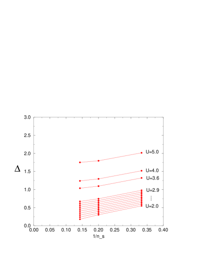
FIG. 18.: The gap $\Delta$ versus the inverse of the number of sites $1/{n_{s}}$ in the paramagnetic insulator for various values of $U$. $\Delta$ is twice the energy of the lowest pole from the ED Green function.

We also investigate the behavior of the inverse moments of the spectral function defined as:

$$m_{-n}=\int_{0}^{\infty}\frac{\rho(\epsilon)d\epsilon}{\epsilon^{n}}$$ (22)

The behavior of these quantities give a more detailed picture of the transition. The local picture of the paramagnetic insulator is that of a spin embedded in an insulator. Hybridization with the bands of this insulator transfers spectral weight to high frequencies but the spin remains well defined at low energies (even though with a reduced spectral weight) as long as there is a finite gap in the insulator. As $U_{c1}$ is approached, and the gap decreases we face the question whether the spin remains well defined even at the transition point. This depends on the behavior of the density of states of the bath $\rho_{bath}$ at low frequecies (we recall, $\rho_{bath}$ is essentially $\rho$ in a Bethe lattice, cf. Eq.6). Whittoff and Fradkin [44] have shown that if the density of states of the bath vanishes as a power-law $\rho_{bath}\propto\epsilon^{\beta}$ the spin remains well defined if $\beta>1$ while the spin is Kondo quenched if $\beta<1$ and the spin degree of freedom is absorbed by the conduction electrons. The case $\beta=1$ is marginal.

In a previous publication [16] we showed that within IPT the second inverse moment remains finite at the transition, while it diverges in the Hubbard III solution.

Notice that $m_{-2}$ can remain finite up to the transition even when the gap closes, but a divergent second inverse moment implies the continuous closure of the gap. In Fig. 19 we plot the inverse of $m_{-2}$ together with that of the first and third inverse moments. The results correspond to the extrapolation to the infinite size effective bath, performed similarly as was done previously for the gap. The inverse of the second inverse moment shows good scaling behavior with the system size and is found to go to zero for $U\approx 2.12$. At this value of the interaction the moment diverges, which signals the breakdown of the insulating state, with the gap closing continuously. As expected, the first inverse moment remains finite at the transition (it also shows good scaling behavior) and, on the other hand, the inverse of the third inverse moment becomes negative even before the transition. This is due to the fast divergence of the third moment which renders the finite size scaling inaccurate. It is important to stress that this way of looking at the transition is very different from the previous one, nevertheless, the estimates for $U_{c1}$ that are obtained after the infinite size bath extrapolation are consistently predicted to within less than 2%. The results are substantially different from the ones obtained from IPT.

FIG. 19.: Inverse of the first three inverse moments $(m_{-n})^{-1}$ of the density of states as a function of $U$. The three curves correspond from top to bottom to the inverse of the first, second and third inverse moment respectively. The results are the $n_{s}\rightarrow\infty$ extrapolation from clusters of 3, 5 and 7 sites assuming ${1}/{n_{s}}$ scaling behavior. The dotted continuation of the last curve indicates results where the scaling is not reliable due to the strong divergent behavior of that inverse moment. The vertical dotted line indicates the value obtained for $U_{c1}$ from the inverse moment analysis.

3 The metallic state.

We now discuss the data in the metallic phase. In Fig.4 at the beginning of this section, we reproduced experimental data for pure samples that become insulating below $T_{c}\approx 150K$ [21]. The spectra were obtained in the metallic phase at $T=170K$ and $T=300K$ and are made up of broad absorption at higher frequencies and some phonon lines in the far infrared. They appear to be rather featureless, however, upon considering their difference (in which the phonons are approximately eliminated) distinct features are observed. As $T$ is lowered, there is an enhancement of the spectrum at intermediate frequencies of order $0.5eV$; and more notably, a sharp low frequency feature emerges that extends from $0$ to $0.15eV$. Moreover, these enhancements result in an anomalous change of the total spectral weight $\frac{\omega_{P}^{2}}{4\pi}$ with $T$. We argue below, that these observations can be accounted by the Hubbard model treated in mean field theory.

In Fig.20 we show the calculated optical spectra obtained from IPT for two different values of $T$. The interaction is set to $U=2.1D$ that places the system in the correlated metallic state. It is clear that, at least, the qualitative aspect of the physics is already captured and setting $D\approx 0.4eV$ we find these results consistent with the experimental data on $V_{2}O_{3}$ (Fig.4). As the temperature is lowered, we observe the enhancement of the incoherent structures at intermediate frequencies of the order $\frac{U}{2}$ to $U$ and the rapid emergence of a feature at the lower end of the spectrum. This two emerging features can be interpreted from the qualitative picture that was discussed in Sec.III which is relevant for low $T$. From the model calculations with the parameters of table I we find the enhancement of the spectral weight taking place at a scale $T_{coh}\approx 0.05D\approx 240K$ which correlates well with the experimental data. $T_{coh}$ has the physical meaning of the temperature below which the Fermi liquid description applies,[16] as the quasiparticle resonance emerged in the density of states.

FIG. 20.: The model $\sigma(\omega)$ for the metallic solution at $U=2.1D$ and $T=0.05D$ (upper) and $0.083D$ (lower). A small $\Gamma=0.3$ and $0.5D$ was included to mimic a finite amount of disorder.

In Fig.21 we present the results for $\langle K\rangle$ as a function of the temperature. An interesting prediction of the model is the anomalous increase of the integrated spectral weight $\frac{\omega_{P}^{2}}{4\pi}$ as $T$ is decreased, a feature that is actually observed in the experimental data (note that the spectral weight is not recovered upto the highest frequencies where experimental data is available ($\omega\approx 6eV$). This effect is due to the rather strong $T$ dependence of the kinetic energy $\langle K\rangle\propto\frac{\omega_{P}^{2}}{4\pi}$ in the region near the crossover indicated by a dotted line in the phase diagram (Fig.5). It results from the competition between two small energy scales, namely, the temperature and the renormalized Fermi energy $\epsilon_{F}^{*}$.

FIG. 21.: Expectation value of minus the kinetic energy $\langle K\rangle$ as a function of the temperature for various $U$ (IPT). This quantity is directly proportional to the optical conductivity sum rule. It predicts a notable increase in the optical spectral weight as the temperature is decreased in the correlated metallic regime.

Fig.22 contains the comparison between the results for the same quantity $\langle K\rangle$ at $U=2$ as obtained from the IPT and the finite temperature ED method. It demonstrates that the temperature dependence is indeed a true feature of the model which is being successfully captured by the approximate IPT solution.

Although the qualitative aspect seems to be very accurately described by the model, we find $\frac{\omega_{P}^{2}}{4\pi}\approx 1000\frac{ev}{\Omega cm}$ which is somewhat lower than the experimental result. This could be due to the contribution from tails of bands at higher energies that are not included in our model, or it may indicate that the bands near the Fermi level are degenerate.

FIG. 22.: Comparison of the expectation value of the kinetic energy $\langle K\rangle$ as a function of the temperature for $U=2$ as obtained from IPT and ED method.

We now want to finally consider an important prediction of the model for the slope of the linear term in the specific heat $\gamma$ in the metallic phase. Experiments show that the slope $\gamma$ is in general unusually large. For $0.08\ Ti$ substitution $\gamma\approx 40\frac{mJ}{molK^{2}}$, while for a pressure of $25Kbar$ in the pure compound $\gamma\approx 30\frac{mJ}{molK^{2}}$ and with $V$ deficiency in a range of $y=0.013$ to $0.033$ the value is $\gamma\approx 47\frac{mJ}{molK^{2}}$.[45] In our model $\gamma$ is simply related to the weight in the Drude peak in the optical conductivity and to the quasiparticle residue $Z$ , $\gamma=\frac{1}{ZD}3\frac{mJeV}{molK^{2}}$. The values of $U=2.1D$ and $D\approx 0.4eV$ extracted from the optical data correspond to a quasiparticle residue $Z\approx 0.3$, and result in $\gamma\approx 25\frac{mJ}{molK^{2}}$ which is close to the experimental findings. Thus, it turns out that the mean field theory of the Mott transition explains in a natural and qualitative manner, the experimentally observed optical conductivity spectrum, the anomalously large values of the slope of the specific heat $\gamma$, and the dc-conductivity in the metallic phase, as consequence of the appearance of a single small energy scale, the renormalized Fermi energy $\epsilon^{*}_{F}$.

B Periodic Anderson model.

1 Gap formation.

A second class of systems where the correlations induce an anomalous temperature dependence are the Kondo insulators. While the most qualitative physics of these systems is well understood, several features remain puzzling [20]. The charge gap $\Delta_{c}$ measured in optical conductivity is larger than the spin gap $\Delta_{s}$ measured in neutron scattering [2]. The transport gap $\Delta_{t}$ obtained from the activation energy in dc-transport measurements is smaller than $\Delta_{c}$. The gap $\Delta_{c}$ begins to open at a characteristic temperature $T^{*}\sim\frac{\Delta_{c}}{5}$ and becomes fully developed at a much smaller temperature of the order of $\frac{T^{*}}{5}$. Also, the gap is temperature independent below $T^{*}$. In $Ce_{3}Bi_{4}Pt_{3}$ it is found that $\Delta_{c}\approx 450K$, $\Delta_{s}\approx 250K$, $T^{*}\approx 100K$ and the optical gap is completely depleted only below $\approx 25K$ [2]. On the other hand, qualitatively similar results were reported for $FeSi$, with $\Delta_{c}\approx 1000K$, $T^{*}\approx 200K$ and the gap becomes depleted between $20$ and $100K$ [3].

The mean field theory accounts for all these observations. The low energy behavior of the one particle Green functions of the model can be understood as that of a non interacting system where the interaction $U$ reduces the hybridization from its bare value $V$ to a renormalized value $V^{*}$ which decreases as $U$ increases. In consequence, the gap in the optical conductivity decreases by the effect of correlations. However, the lineshape remains approximately invariant, and merely changed by a rescaling factor respect to the response of the non-interacting model. This is demonstrated by the plot of the optical conductivity $\sigma(\omega)$ for different values of $U$ shown in Fig.23. The optical gap $\Delta_{c}$ is given by the direct gap $\Delta_{dir}$ of the renormalized band structure. These results were obtained by IPT at $T=0$ and we checked in various cases that the results are in excellent agreement with the ED method.

FIG. 23.: The optical conductivity spectra of the periodic Anderson model for values of the interaction $U=0.5,1,2,3$ (right to left), keeping the hybridization $V=0.25$ fixed. The inset shows the gap from the optical spectra $\Delta_{c}\approx\Delta_{dir}$ and the indirect gap $\Delta_{ind}$ from the local density of states for $V=0.6$. The slopes of these curves indicate that ${V^{*}}^{2}/D\propto\Delta_{ind}$ and $V^{*}\propto\Delta_{dir}$ in the strong correlation region.

We now consider the behavior of $\sigma(\omega)$ with temperature. Fig.24 shows the optical conductivity for different temperatures with the parameters $U=3$ and $V=0.25$ fixed. The gap is essentially temperature independent. It begins to form at $T^{*}\approx 0.02\sim\frac{\Delta_{c}}{5}$, and is fully depleted only at temperatures of the order of $\frac{T^{*}}{5}$. We thus observe that the mean field theory is able to capture the qualitative aspect of the experimental results that we summarized before. This basically consists in the individualization of 3 different energy scales: the largest corresponds to the gap of the optical spectra $\Delta_{c}\sim\Delta_{dir}$, an intermediate scale $T^{*}\sim\frac{\Delta_{c}}{5}$ where this gap starts to form and quasiparticle features start to appear in the $DOS$ and, a third and smaller scale $\Delta_{ind}\sim\frac{T^{*}}{5}$, which corresponds to the temperature where the optical gap gets completely depleted. As demonstrated in Fig.25 where we plot the results for the density of states, that smallest scale $\Delta_{ind}$ also indicates the temperature below which the gap in the density of states opens, and, thus, can be associated to the gap measured in dc-transport experiments $\Delta_{t}$.

FIG. 24.: The optical conductivity for the Anderson model at $T=0.001$ (bold), $0.005,0.01,0.02$ (dotted), $0.03$ (thin). The interaction $U=3$ and $V=0.25$. Inset: The same quantity at $T=0.001$ (bold), $0.005,0.01,0.02$ (dotted), $0.03$ (thin) with lorentzian random site disorder of width $\Gamma=0.05$.

FIG. 25.: Low frequency part of the density of states for the $d$ and $c-$electrons (top and bottom) obtained from IPT at $T$ = 0.001, 0.005, 0.01, 0.02, 0.03 for $U=3$ and $V=0.25$ (top to bottom for $d-$electrons and bottom to top for $c-$electrons). Inset: The density of states in the full frequency range at $T\ =\ 0.001$.

In order to make a meaningful comparison with the experimental data, we have added the effects of disorder by putting a lorentzian distributed random site energy on the conduction electron band with width $\Gamma=0.05$. The results are displayed in the inset of Fig.24 and they show that the introduction of disorder makes the overall shape of the spectra in closer agreement with the experimental results [2, 3] (for a discussion of the scattering involved, see subsection IV B 2). Also, we observe that increasing the disorder reduces the temperature $T^{*}$.

In the following, we briefly address the question of the integrated total spectral weight. It has been noticed that the experimental results in both, $Ce_{3}Bi_{4}Pt_{3}$ and $FeSi$, seem to violate the sum rule for the spectral weight [2, 3]. However, this point has been recently questioned, at least for the $FeSi$ compound [46]. In order to contribute to the proper interpretation of the experimental data, it is important to compute the kinetic energy of our model at finite temperature, which is directly related to the sum rule of Eq.16. The results from IPT are presented in Fig.26 which shows the notable dependence of the kinetic energy with temperature and interaction strength (we plot the negative of $\langle K\rangle$ which is the quantity that enters Eq.16). In Fig.27, we plot similar results obtained with the ED algorithm which demonstrates that the behavior captured by the IPT calculation is indeed a true feature of the model.

FIG. 26.: Expectation value of minus the kinetic energy $\langle K\rangle$ as a function of the temperature for $U=0,2,3,4$ and $V=0.4$ (bottom to top) as obtained from (IPT). This quantity is directly related to the optical conductivity sum rule. It predicts a notable decrease in the total optical spectral weight as the temperature is decreased in the range below the maxima.

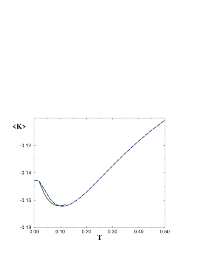
FIG. 27.: Comparison of the expectation value of the kinetic energy $\langle K\rangle$ in the PAM as a function of the temperature for $U=2$ and $V=0.4$ as obtained from IPT and ED method (dashed line and full line).

As we have previously discussed for the the Hubbard model case, the strong correlation effects that renders $\langle K\rangle$ a function of the temperature implies that if the PAM is the relevant model for the systems at low energies, then the results predict the behavior of the integrated optical weight within the low frequence range. Actually, experimental data which is inferred from the Kramers-Kronig transformation of reflectivity measurements, can only be reliably obtained within a limited low frequency range of the order of a few $eV$. The behavior of $\langle K(T)\rangle$ in Fig.27 is non-monotonic. As we increase the temperature from zero, we observe that initially the kinetic energy decreases. This is a consequence of the electron delocalization since the system becomes a metal as the small gap in the density of states is filled. The kinetic energy then goes through a minimum and starts to increase as the temperature is further increased. This is simply due to the thermal excitation of electrons within the single conduction band. Correlations now play an irrelevant role as the temperature is higher than the coherence temperature $T^{*}$. When we study the behavior for different values of the interaction $U$ in Fig.26, we observe that the position of the minima (maxima in this figure as $-\langle K(T)\rangle$ is plotted), becomes smaller as $U$ is increased. This can be understood simply as a consequence of the renormalization of the hybridization amplitude $V\rightarrow V^{*}$.

In regard to the experimental situation in the Kondo insulators, which indicate the apparent violation of the optical sum rule, our results give a plausible qualitative explanation for the observed behavior. In fact, for experimental data obtained at temperatures smaller than the size of the gap $\Delta_{c}$ and restricted to a finite low frequency range (which is in fact the actual situation), the model predicts the apparent “disappearance” of spectral weight as the temperature is decreased.

We should also point out that although this simple model accounts, rather successfully, for the various energy scales, it fails to provide an accurate reproduction of the detailed experimental lineshape. A complete explanation of the experimental results may need the consideration of additional sources of scattering, as will be discussed in the next subsection.

To finish our discussion on the gap formation in the periodic Anderson model we shall present the results for the size of the various gaps that are obtained from the correlation functions.

The first study of the periodic Anderson model in large dimensions was carried out by Jarrell et al. using quantum Monte Carlo [22]. Our spectral functions and density of states are in general agreement with the early work in the region where the QMC and exact diagonalization method can be compared. A noticeable qualitative difference is that we find the spin gap to be slightly but strictly smaller than the indirect gap when $U\neq 0$.

In Fig.28 we show the local spin and charge correlation functions along with the optical conductivity which shows the qualitative agreement with the experimental data of Ref.[2]. We also compare in the inset the direct optical gap $\Delta_{dir}$, the indirect gap $\Delta_{ind}$ relevant for transport properties, and the spin gap $\Delta_{s}$ obtained from the spin-spin correlation function. We find that $\Delta_{dir}$ is consistently larger than $\Delta_{s}$, and that $\Delta_{s}$ is somewhat smaller than $\Delta_{ind}$. As expected when $U=0$, $\Delta_{s}=\Delta_{ind}$, but as $U$ increases $\frac{\Delta_{s}}{\Delta_{ind}}$ becomes smaller than unity and approaches the value $1/2$ at $U\approx 2$.

FIG. 28.: The local spin-spin (bold) and charge-charge (thin) susceptibility from 7 sites ED. The optical conductivity from IPT (dotted). The parameters are $U=1$ and $V=0.2$. The y-axis is in arbitrary units. Inset: The direct gap form IPT (upper dotted line), the indirect gap (lower dotted line) and the spin gap (solid line) from 8 sites ED. The hybridization is $V=0.2$.

2 The scattering rate.

In the previous section we have stressed the qualitative success of the mean field theory of the periodic Anderson model in connection with the gap formation in Kondo insulators like $FeSi$ and $Ce_{3}Bi_{4}Pt_{3}$. In this section, however, we will show that this approach cannot account for the large scattering rate measured in these materials, if one does not include the effects of disorder in the model. This is very surprising and is an indication of the limitations of the one band periodic Anderson model for modeling these systems.

The optical conductivity of Kondo insulators is – except for the gap which forms at low temperatures – almost constant over a large frequency range extending to several times the width of the gap. The corresponding value of $\sigma(\omega)$ is quite similar for all of the materials (typically 3000 - 4000 $(\Omega cm)^{-1}$ ) and depends only weakly on temperature. The related scattering rate can be estimated (at $T>T^{*}$) by simple Drude model arguments: at zero frequency, we have $\sigma=\frac{ne^{2}\tau}{m}$. Here, $n=a^{-3}$, where $a$ denotes the lattice constant. $m$ can be obtained from the kinetic energy $\frac{p^{2}}{2m}\approx D$, where $p\approx\frac{2\pi\,\hbar}{a}$. Assuming $a\approx 10^{-10}m$, the equations yield $\hbar/\tau\sim\sigma_{0}^{-1}10^{3}(\Omega cm)^{-1}D$. Thus the measured values for $\sigma_{0}$ imply a scattering rate which is of the order of the bandwidth ($\frac{1}{\tau}\sim D$, assuming $\hbar=1$). This should be compared with the scattering rate found in normal metals like copper, which is three orders of magnitude smaller ($\frac{1}{\tau}\sim 10^{-3}D$).

Since all experiments on Kondo insulators (and also on many Kondo metals) observe (above the gap) the same order of magnitude for $\sigma(\omega)$ one should expect that there is a common mechanism involved. It is reasonable to assume that the scattering of conduction electrons by the localized electrons in the periodic Anderson model provides an explanation. To address this question, we calculated the effective scattering rate. This quantity is determined by the effective c-electron self-energy $\Sigma_{cc}^{(eff)}$

$$\Sigma_{cc}^{(eff)}(\omega)=\frac{V^{2}}{\omega+\mu-\Sigma_{dd}(\omega)},$$ (23)

where $\Sigma_{dd}$ is the self-energy of the localized $d-$electrons, which enters the formula for the optical conductivity (15) via $A_{\epsilon_{k}}(\omega)=-2\,\mbox{Im}\frac{1}{\omega+\mu-\epsilon_{k}-\Sigma^{(eff)}_{cc}(\omega)}$. The imaginary part of $\Sigma_{cc}^{(eff)}(\omega)$ measures the scattering involved. In Fig.29 we plotted this quantity for the particle hole symmetric case, $V=0.25D$, $U=3D$, and $T=0.1D$. Since in this section we are not interested in the gap formation the temperature was chosen to be well above the point where the gap starts to open ($T^{*}\approx 0.025D$). For comparison, the calculation was done with both ED and IPT.

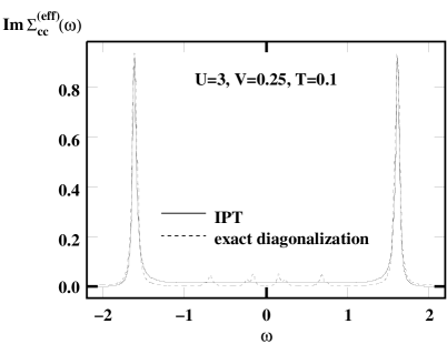
FIG. 29.: $\mbox{Im}\Sigma^{(eff)}_{cc}(\omega)$ for $U=3$, $V=0.25$, and $T=0.1$ ($D=1$). The results are from ED (dashed line) and IPT (full line).

It is clear from the plot that the scattering rate is much smaller than the bandwidth $D$ and gives rise to an optical conductivity which is smaller than the experimentally observed value by two orders of magnitude. This result remains valid away from particle hole symmetry and for different choices of $V$ and $U$. If one ignores the self consistency condition, one would expect, based on the theory of the Kondo impurity model that as the temperature is lowered the scattering rate should grow towards the unitary limit, $D$ , this growth, which is expected at low frequencies and low temperatures is preempted, in the lattice by the formation of the hybridization gap.

For $\frac{V}{U}\ll 1$ and half filling, the periodic Anderson model can be transformed into a Kondo lattice model by a Schrieffer-Wolff Transformation:

$$H_{KL}=\frac{D}{2}\sum_{<ij>,\sigma}c^{\dagger}_{i\sigma}\,c_{j\sigma}+J\,\sum_{i,\sigma\sigma^{\prime}}\vec{S}_{i}\,c^{\dagger}_{i\sigma}\vec{\tau}_{\sigma,\sigma^{\prime}}c_{i\sigma^{\prime}}$$ (24)

where $J\,=\,8\,\frac{V^{2}}{U}$. Here, $\vec{S}_{i}$ describes a spin at site $i$. For a cross-check, we also examined this hamiltonian using the exact diagonalization method. For $J=\frac{1}{6}\,D$, which corresponds to $V=0.25\,D$ and $U=3\,D$, we find at $T=0.1\,D$ a scattering rate $\frac{1}{\tau}\sim-\mbox{Im}\Sigma_{cc}(\omega=0)\approx 7\times 10^{-3}D$. This is again much less than required to explain the experimental data.

We believe that the failure observed here within the present approach is a general shortcoming of the periodic Anderson model. A more realistic description has to take several crystal filed split bands and this could increase the finite frequency optical absortion.

V Conclusions.

In this paper we have illustrated how the LISA, that becomes exact in the limit of large dimensions, can be used to study the physics of systems where the local interactions are strong and play a major role. In particular we have demonstrated that the Hubbard and the periodic Anderson model treated within this dynamical mean field theory can account for the main features of the temperature dependent transfer of spectral weight in the optical conductivity spectra. In the case of $V_{2}O_{3}$ we found that the theory is able to account semi-quantitatively for the conductivity results in both the metallic and insulating states. In the former case it can also account for the topology and energy scales of the experimental phase diagram as well as for the unusually big values observed in the slope of the specific heat $\gamma$. In the latter case, the theory seems to provide further insights in the role of the magnetic frustration. In this regard, we have studied in detail the predictions of the model for photoemission spectra in the insulating phase with long range order and noted that the present mean field theory indeed captures many aspects of the behavior encountered in the numerical studies of the model in low dimensions.

For the Kondo insulators, we have seen most of the qualitative features of the observed behavior of optical spectra with temperature being captured in detail by our model treated in mean field theory. In particular we identified the different energy scales that describe the thermal filling of the optical gap and how they relate to the changes in the single particle spectra. However, we saw that the periodic Anderson model is not able to explain the high scattering rate measured in Kondo insulators.

We presented results for the temperature dependence of the optical sum rule in the strongly correlated models. While in the Hubbard case, the results capture the qualitative change of the total spectral weight with temperature observed in the $V_{2}O_{3}$ system, our quantitative results on the PAM may be relevant for the resolution of the “missing” spectral weight controversy in optical experiments on the insulators $Ce_{3}Bi_{4}Pt_{3}$ and $FeSi$ [2, 3, 46]. From a broader perspective it has turned out to be very illuminating to realize how the emergence of a small “Kondo” energy scale which is a correlation effect results in an unusual temperature dependence of the projected optical sum rule (cf. Eq.16) in the Hubbard and the periodic Anderson model. We have shown that in the former case the optical weight increases when the temperature is reduced and the system becomes more metallic, while in the latter it decreases, as a consequence of the system opening a gap and becoming insulating.

We finally stress that our mean field approach can be easily adapted to incorporate more realistic band structure density of states and more complicated unit cells. These extensions would allow for a more precise quantitative description of these interesting systems.

A Addition of two continued fractions.

In this appendix we present an algorithm that allows to sum two continued fractions into a single one. This is necessary for the implementation of the ED method in models with magnetic frustration or disorder, where various Green functions have to be averaged and the result has to be expressed as a new continued fraction. The details of the ED method can be found in Ref.[18].

In the ED method an effective cluster hamiltonian $H^{n_{s}}$ of $n_{s}$ sites is diagonalized. At $T=0$ only the groundstate $|gs\rangle$ and the groundstate energy $E_{0}$ need to be obtained, and this can be efficiently done by the modified Lanczos method.[47] The local Green function $G(\omega)$ is then obtained as a continued fraction. Actually one needs to compute two continued fractions $G^{<}(\omega)$ and $G^{>}(\omega)$, for $\omega<0$ and for $\omega>0$ respectively.

$$G(\omega) = G^{>}(\omega)+G^{<}(\omega)$$ (A1)

$$= \langle gs|c\frac{1}{\omega-(H^{n_{s}}-E_{0})+i\delta}c^{\dagger}|gs\rangle$$ (A3)

$$+\langle gs|c^{\dagger}\frac{1}{\omega+(H^{n_{s}}-E_{0})+i\delta}c|gs\rangle$$

with

$$G^{>}(\omega)=\frac{\langle gs|cc^{\dagger}|gs\rangle}{\omega-a_{0}^{>}-\frac{b_{1}^{>2}}{\omega-a_{1}^{>}-\frac{b_{2}^{>2}}{\omega-a_{2}^{>}-...}}}$$ (A4)

(A5)

$$G^{<}(\omega)=\frac{\langle gs|c^{\dagger}c|gs\rangle}{\omega-a_{0}^{<}-\frac{b_{1}^{<2}}{\omega-a_{1}^{<}-\frac{b_{2}^{<2}}{\omega-a_{2}^{<}-...}}}$$ (A6)

where $c$ and $c^{\dagger}$ are the operators associated with the local site of $H^{n_{s}}$. The parameters $a_{i}^{>/<}$ and $b_{i}^{>/<}$ define the continued fractions and are obtained from the following iterative procedure,

$$a_{i}^{\alpha}=\langle f_{i}^{\alpha}|H^{n_{s}}|f_{i}^{\alpha}\rangle,\ \ \ \ \ \ {b_{i}^{\alpha}}^{2}=\frac{\langle f_{i}^{\alpha}|f_{i}^{\alpha}\rangle}{\langle f_{i-1}^{\alpha}|f_{i-1}^{\alpha}\rangle}$$ (A7)

where $\alpha=>,<$ and $|f_{0}^{>}\rangle=c^{\dagger}|gs\rangle$, $|f_{0}^{<}\rangle=c|gs\rangle$ and

$$|f_{i+1}^{\alpha}\rangle=H^{n_{s}}|f_{i}^{\alpha}\rangle-a_{i}^{\alpha}|f_{i}^{\alpha}\rangle-{b_{i}^{\alpha}}^{2}|f_{i-1}^{\alpha}\rangle$$ (A8)

and in the beginning we set $b_{0}^{\alpha}=0$.

Thus, we observe that the basis defined by the vectors $|f_{i}^{\alpha}\rangle$ gives a tri-diagonal representation of $H^{n_{s}}$ which contains the $a_{i}$’s along the main diagonal and the $\sqrt{b_{i}}$’s along the diagonals next to the main one. In the following we drop the index $\alpha$ to simplify the notation. We will explicitly restore it in the final result.

Let’s now address the problem of our current interest. We assume that we have computed two Green functions $G_{\mu}(\omega)$ where the index $\mu$ may label, for instance, a spin. Our task is to obtain a new continued fraction representation of the average Green function $\bar{G}(\omega)=\frac{1}{2}(G_{\uparrow}(\omega)+G_{\downarrow}(\omega))$. The more general case of a weighted average can be trivially generalized from the present case which we consider for simplicity.

We first note that, from the Lanczos procedure, $H^{n_{s}}$ has (different) tri-diagonal representations in the two sub-basis defined by $|f_{i\mu}\rangle$ (we have dropped the $>,<$ label to simplify notation). The representation is basically a matrix that contains the parameters $a^{\prime}s$ along the main diagonal and the $b^{\prime}s$ along the two sub-diagonals.

The algorithm is as follows: one first diagonalizes the two tri-diagonal representations of $H^{n_{s}}$ by computing all the eigenvalues and eigenvectors. This is not numerically costly since the matrices are in tri-diagonal form and it may be done by standard methods.

An important result that can be easily demonstrated is that the eigenvalues $\epsilon_{\mu}^{\nu}$ of the tri-diagonal matrices are the poles of their corresponding Green functions $G_{\mu}(\omega)$. Furthermore, one can also show that

$$G_{\mu}(\omega)=\sum_{\nu=1}^{M}{\frac{({v^{\nu}_{\mu}})^{2}}{\omega-\epsilon^{\nu}_{\mu}}}$$ (A9)

where $v^{\nu}_{\mu}$ are the first component of the $M$ eigenvectors of the tri-diagonal matrices.

Thus, from the definition of the Green function, one immediately recognizes that the vector {$v^{1}_{\mu},v^{2}_{\mu},...,v^{M}_{\mu}$} is nothing but $c^{\dagger}_{\mu}|gs\rangle$ expressed in a basis where $H^{n_{s}}$ is diagonal (which is a sub-basis of the given sector’s Hilbert space).

The final step consists in writing the hamiltonian in the basis direct product of the two sub-basis, which, of course, will also be a diagonal representation of $H^{n_{s}}$; and then bring it to its tri-diagonal representation through the steps (A7), (A8) starting from the vector defined by (restoring the $>,<$ label)

$$|f_{0}^{>}\rangle = (c^{\dagger}_{\uparrow}+c^{\dagger}_{\downarrow})|gs\rangle$$ (A10)

$$= \vec{v}_{\uparrow}\oplus\vec{v}_{\downarrow}$$ (A11)

$$= \{v^{1}_{\uparrow},v^{2}_{\uparrow},...,v^{M}_{\uparrow},v^{M+1}_{\downarrow},v^{M+2}_{\downarrow},...,v^{2M}_{\downarrow}\}$$ (A12)

Thus, the newly determined $a_{i}^{>}$’s and $b_{i}^{>}$’s that result from this last step are the parameters of the continued fraction representation of $\bar{G}^{>}(\omega)$ (the parameters for $\bar{G}^{<}$ are obtained in a completely analogous manner).

REFERENCES

- [1] G. A. Thomas et al. Journ. Low Temp. Phys. 95, 33 (1994).
- [2] B. Bucher, Z. Schlesinger, P. C. Canfield and Z. Fisk, Phys. Rev. Lett. 72, 522 (1994). B. Bucher et al., Physica B 199200, 489 (1994).
- [3] Z. Schlesinger, Z. Fisk, H. T. Zhang, M. B. Maple, J. F. DiTusa and G. Aeppli, Phys. Rev. Lett. 71, 1748, (1993).
- [4] M. A. van Veenendaal and G. A. Sawatzky Phys. Rev. Lett. 70, 2459 (1993); Phys. Rev. B 49, 3473 (1994).
- [5] A. J. Millis, in Physical Phenomena at High Magnetic Fields, edited by E. Manousakis et al. (Addison-Wesley, Reading, MA, 1991); and references therein.
- [6] For a recent review see A. Georges, G. Kotliar, W. Krauth and M. J. Rozenberg, Rev. Mod. Phys. (to appear 1996).
- [7] W. Metzner and D. Vollhardt Phys. Rev. Lett. 62, 324 (1989).
- [8] A. Georges and G. Kotliar, Phys. Rev. B 45, 6479 (1992).
- [9] A. Georges, G. Kotliar and Q. Si Int. J. Mod. Phys. B 6, 705 (1992).
- [10] M. Jarrell, Phys. Rev. Lett. 69, 168 (1992).
- [11] M. J. Rozenberg, X. Y. Zhang and G. Kotliar, Phys. Rev. Lett. 69, 1236 (1992).
- [12] A. Georges and W. Krauth, Phys. Rev. Lett. 69, 1240 (1992).
- [13] X. Y. Zhang, M. J. Rozenberg and G. Kotliar, Phys. Rev. Lett. 70, 1666 (1993).
- [14] Th. Pruschke, D. L. Cox and M. Jarrell, Phys. Rev. B 48, (1993).
- [15] A. Georges and W. Krauth, Phys. Rev. B 48, 7167 (1993).
- [16] M. J. Rozenberg, G. Kotliar and X. Y. Zhang Phys. Rev. B 49, 10181 (1994).
- [17] M. Caffarel and W. Krauth Phys. Rev. Lett. 72, 1545 (1994).
- [18] Q. Si, M. Rozenberg, G. Kotliar and A. Ruckenstein Phys. Rev. Lett. 72, 2761 (1994); M. J. Rozenberg, G. Moeller, and G. Kotliar, Mod. Phys. Lett. B 8, 535 (1994).
- [19] G. Moeller, Q. Si, G. Kotliar, M. Rozenberg and D. Fisher Phys. Rev. Lett. 74, 2082 (1995).
- [20] G. Aeppli and Z. Fisk, Comments Cond. Mat. Phys.16, 155 (1992).
- [21] M. J. Rozenberg, G. Kotliar, H. Kajueter, G. A. Thomas, D. H. Rapkine,J. M. Honig, and P. Metcalf, Phys. Rev. Lett. 75, 105 (1995).
- [22] M. Jarrell, H. Akhlaghpour and Th. Pruschke, Phys. Rev. Lett. 70, 1670 (1993); see also, D. Hirashima and T. Mutou, Physica B 199200, 206 (1994).
- [23] Th. Pruschke, D. L. Cox, and M. Jarell, Europhys. Lett. 21 (5), 593, (1993)
- [24] P. F. Maldague, Phys. Rev. B, 16, 2437 (1977).
- [25] W. Kohn, Phys. Rev. A171, 133 (1964).
- [26] D. Baeriswyl, C. Gros, and T. M. Rice, Phys. Rev. B, 35, 8391 (1987).
- [27] Anil Khurana, Phys. Rev. Lett. 64, 1990 (1990).
- [28] P. Coleman, Phys. Rev. B 29, 3035 (1984). T. M. Rice and K. Ueda, Phys. Rev. B 34, 6420 (1986).
- [29] M. J. Rozenberg, Phys. Rev. B (to appear September 1995).
- [30] C. Castellani, C. R. Natoli, and J. Ranninger, Phys. Rev. B 18, 4945 (1978).
- [31] L. F. Mattheiss, J. Phys., Condens. Matter 6, 6477 (1994).
- [32] J. H. Park, L. H. Tjeng, J. W Allen, P. Metcalf and C. T. Chen, ATT Bell Labs Report, (1994).
- [33] H. Kuwamoto, J. M. Honig, and J. Appel, Phys. Rev. B 22, 2626 (1980).
- [34] D. Mc Whan et al., Phys. Rev. B 7, 1920 (1973).
- [35] S. A. Carter, T. F. Rosenbaum, J. M. Honig, and J. Spalek, Phys. Rev. Lett. 67, 3440 (1992).
- [36] For details on the application the theory to models with long range order see Ref.[9], [16] and [29].
- [37] J. Hubbard, Proc. Roy. Soc. (London) A281, 401 (1964).
- [38] S. Shin et al., J. Phys. Soc. Jpn. 64, 1230-1235 (1995).
- [39] A. Matsuura et al. (preprint, 1994).
- [40] A. Moreo, S. Haas, A. Sandvik, and E. Dagotto (unpublished 1995).
- [41] R. Preuss, W. Hanke, and W. von der Linden, Phys. Rev. Lett. 75, 1344 (1995).
- [42] G. A. Thomas et al., Phys. Rev. Lett. 73, 1529 (1994).
- [43] R. M. Moon, Phys. Rev. Lett. 25, 527 (1970).
- [44] D. Whittoff and E. Fradkin, Phys. Rev. Lett. 64, 1835 (1990).
- [45] D. Mc Whan et al., Phys. Rev. Lett. 27, 941 (1971); D. Mc Whan et al., Phys. Rev. B 7, 3079 (1973); S. A. Carter, T. F. Rosenbaum, P. Metcalf, J. M. Honig, and J. Spalek Phys. Rev. B 48, 16841 (1993).
- [46] L. Degiorgi et al., Europhys. Lett. 28 (5), 341-346 (1994).
- [47] E. Gagliano et al., Phys. Rev. B 34, 1677 (1986).