On the Statistical Properties of the Large Time Zero Temperature Dynamics of the SK Model

Abstract

In this note we study the zero temperature dynamics of the Sherrington Kirkppatric model and we investigate the statistical properties of the configurations that are obtained in the large time limit. We find that the replica symmetry is broken (in a weak sense). We also present some general considerations on the synchronic approach to the off-equilibrium dynamics, which have motivated the present study.

1 Introduction

In recent years there have been many progresses in our understanding of the non-equilibrium dynamics [2]-[7] of the infinite Sherrington Kirkpatrick model [8, 9] and of other glassy systems [10, 11, 12]. The aim of these studies is to compute the properties of the systems (e.g. the energy or the magnetization) as function of time if we know the initial configuration at time zero.

These progresses have been done using a diachronic approach in which the evolution of the system is studied by writing closed equations for the correlation functions and response functions at different times.

An alternative synchronic approach has been put forward [13, 14]; here we consider the probability distribution of the configurations of the system at a given time $t$ ($P_{t}(\sigma))$ and we write it as

$$P_{t}(\sigma)\propto\exp(-{\cal H}_{t}(\sigma)).$$ (1)

In this approach there are two crucial steps:

• (a) The determination of the effective Hamiltonian ${\cal H}_{t}$. It is possible that in order to obtain qualitative and semiquantitative information it is not necessary to compute exactly ${\cal H}_{t}$, and an approximate knowledge is sufficient.

• (b) The computation of the statistical properties of the system at given effective Hamiltonian.

This approach may be successfully only if the effective Hamiltonian ${\cal H}_{t}$ (or a reasonable approximation to it) is not too complicated. While the diachronic approach is rather systematic, a good amount of guesswork is needed in the synchronic approach in order to chose a reasonable form of the effective Hamiltonian.

In order to get some intuition on the possible forms of the effective Hamiltonian we have studied in this note the statistical properties of the configurations that are obtained at large times in the SK model using a zero temperature dynamics. This problem has already been studied in the past [5, 7, 15, 16, 17, 18], and it has its own interest. We have obtained some new and unexpected results, i.e. we have found that the replica symmetry is broken (in a weak sense [19, 20]) and that the distribution of the local fields has uneexpected properties.

In the second section we present some general considerations on the synchronic approach. These considerations have been the motivation of the present study, but they may be skipped by the reader interested only in the results of the paper for the SK model. In the third section we define the dynamics which we study and we recall some known results on the zero temperature solutions of the TAP equations [21]. In section IV we present the numerical results of our investigations and finally in the last section we present some tentative conclusions.

2 The Synchronous Approach

We consider a system whose variables satisfy some kind of stochastic or deterministic evolution equations.The probability distribution of the configurations at time zero is given:

$$P_{0}\propto\exp(-{\cal H}_{0}).$$ (2)

The quantity ${\cal H}_{0}$ plays the role of boundary condition.

In the simplest case the system is random at time zero and ${\cal H}_{0}=0$. Our aim is to compute ${\cal H}_{t}$ given ${\cal H}_{0}$. If we are rather luckily we can compute it exactly. This happens for example in the Gaussian SK [14] or in the spherical SK model. Before discussing the general approach it may be useful to show in details the soluble example.

2.1 The Gaussian Sherrington Kirkpatrick model

In the Gaussian Sherrington Kirkpatrick [14] the Hamiltonian is

$$H=-\sum_{i,k}J_{i,k}\sigma_{i}\ \sigma_{k},$$ (3)

where the variables $\sigma_{i}$ are real, with an intrinsic probability distribution at infinite temperature equal to the product of uncorrelated Gaussian of unit variance.

The variables $J_{i,k}$ are usually Gaussian distributed and uncorrelated. The precise form of the distribution of variable $J$ is not important here; we will only assume for simplicity of notations that the matrix $J$ does not have zero eigenvalues.

The dynamic is given by the Langevin equation:

$${d\sigma_{i}\over dt}=-\sigma_{i}+\beta F_{i}(t)+\eta_{i}(t),$$ (4)

where the force is given by

$$F_{i}(t)=-{\partial H\over\partial\sigma_{i}}=\sum_{k}J_{i,k}\sigma(t)_{k}.$$ (5)

The variables $\eta$ are have an uncorrelated white noise distribution

$$\langle\eta_{i}(t)\eta_{k}(t^{\prime})\rangle=2T\delta(t-t^{\prime})\delta_{i,k}.$$ (6)

We suppose that at time zero the initial condition is simply $\sigma(0)_{i}=0$. It is easy to show that the effective Hamiltonian at time $t$ is given by

$${\cal H}_{t}(\sigma)=\sum_{i,k}\sigma_{i}f^{t}(J)_{i,k}\sigma_{k},$$ (7)

where the function $f^{t}$ is given by

$$f^{t}(z)={z\over 1-\exp(-tz)}$$ (8)

and $f^{t}(J)_{i,k}$ denote the $i,k$ element of the matrix $f^{t}(J)$.

The proof of this statement may be obtained by noticing that the evolution equations becomes much simpler in the basis where the matrix $J$ is diagonal [14, 22, 23]. In this basis it is easy to see that the components of the variables $\sigma$ along the eigenvectors of the matrix $J$ are uncorrelated. Their variance can be computed and in this way one obtains equation (8).

2.2 The general approach

In the general case the system has an Hamiltonian $H_{J}(\sigma)$ and the evolution is described by a Langevin equation of the form in eq. (4) or by some analogous equation for discrete systems.

We suppose that the effective Hamiltonian can be written as

$${\cal H}_{0}=g(\sigma,J,\lambda(t)),$$ (9)

where $g$ is a preassigned function which depend on $M$ variables $\lambda_{\alpha}(t)$ ($\alpha=1...M$); $M$ may also be infinite. In this framework the effective Hamiltonian depends on time only trough the variables $\lambda(t)$.

If we suppose to know the function $g$ (or a good approximation to it), the problem consists in finding the appropriate values of the functions $\lambda_{\alpha}(t)$.

There are two strategies which we can follow:

• (a) We choose a set of observables $O_{\alpha}(\sigma,J)$ for $\alpha=1...M$ and we impose the validity of the equations:

  $${d\langle O_{\alpha}\rangle_{t}\over dt}=\sum_{\gamma}{\partial\langle O_{\alpha}\rangle_{t}\over\partial\lambda_{\gamma}}{d\lambda_{\gamma}\over dt},$$ (10)

  where the r.h.s. is computed using the Langevin equatios.

  If we are new to equilibrium it is convenient to write

  $${\cal H}_{t}=\beta H+\sum_{\gamma}O_{\gamma}\lambda_{\gamma}(t).$$ (11)

  For small values of $\lambda_{\gamma}(t)$ we can linearize the equations and we get

  $$\sum_{\gamma}\langle O_{\alpha}O_{\gamma}\rangle_{c}{d\lambda_{\gamma}(t)\over dt}=\sum_{\gamma}\langle\sum_{i}{\partial O_{\alpha}\over\partial s_{i}}{\partial O_{\gamma}\over\partial s_{i}}\rangle\lambda_{\gamma}(t),$$ (12)

  where the expectation values are computed at equilibrium and $\langle\rangle_{c}$ denotes the connected expectation value.

• (b) We write down the Fokker Plank equation:

  $${dP\over dt}={\cal L}P(T),$$ (13)

  where ${\cal L}$ is the appropriate linear operator. A variational principle may be used to chose the variables $\lambda_{n}(t)$. For example we can impose that

  $$\sum_{\{\sigma\}}(\sum_{\gamma}{\partial P(t)\over\partial\lambda_{\gamma}}{d\lambda_{\gamma}\over dt}-{\cal L}P(t))^{2}$$ (14)

  takes the minimum value.

In the past this point of view has been advocated in the study of turbulence and both strategies have been followed [24, 25].

In their original work Cooley and Sherrington [13] have analysed the dynamics of the SK model with Ising spins. They have taken $M=2$. In the case of all spins equal to 1 at time zero, they have

$$g(\sigma,J,\lambda(t))=\lambda_{1}(t)\sum_{i,k}J_{i,k}\sigma_{i}\sigma_{k}+\lambda_{2}(t)\sum_{i}\sigma_{i}$$ (15)

Reasonable results have been obtained expecially at the short times.

It is clear that the previous equation (with (M=2)) is only a first approximation. In the case of the Gaussian SK model it was proved [14] that it does not reproduce the exact result. Indeed in this last case we have seen that the correct expression (for $\sigma_{i}(0)=0$) is given by

$$g(\sigma,J,\lambda(t))=\sum_{\alpha=1,\infty}\lambda_{\alpha}(t)\sum_{i,k}(J^{\alpha})_{i,k}\sigma_{i}\sigma_{k},$$ (16)

where as usual $(J^{\alpha})_{i,k}$ is the matrix element of the matrix $J$ to the power $\alpha$.

For the Ising case is possible that the previous formula is not adequate and that other terms may be present as

$$\sum_{i}\sigma_{i}(\sum_{k}J_{i,k}\sigma_{k})^{3}.$$ (17)

It is quite reasonable that near to the critical temperature too high powers of the variables $\sigma$ are not present so that it possible that a manageable approximation may be done using the techniques developed in [12].

3 Zero temperature dynamics and the TAP equations

Here we consider the SK Ising model with the Hamiltonian in eq. (3), with the $J$ random independent Gaussian variables with variance ${1\over N}$, $N$ being the total number of Ising spins. We study later the case where the variables $J$ take the values $\pm N^{-1/2}$. The two models coincide in the limit $N\to\infty$.

We are interested in studying the statistical properties of the configurations that are obtained by the dynamics at zero temperature at large times. In this case the dynamics is such to orient the spins with the effective field $h_{i}=\sum_{k}J_{i,k}\sigma_{k}$. In other words one set

$$\sigma_{i}(t+1)=\mbox{sign}(h_{i}(t)).$$ (18)

Different algorithms differs in the order in which the rule eq. (18) is applied.

The algorithm stops when in all the sites the following equation is satisfied

$$\sigma_{i}(t)=\mbox{sign}(h_{i}(t)).$$ (19)

The asymptotic configuration at large times depend on the initial configuration. We are interested in studied the ensemble in which the each solution of zero temperature TAP equation (19) is weighted with the probability of being obtained by the algorithm with a random choice of the initial configuration. In other words we weight each solution with the size of its attraction basin.

It is known that in the large $N$ limit the energy density of the asymptotic configuration does not depend on the stating configuration with probability one and it is higher that the ground state energy. Indeed for a sequential algorithm it is about $E_{S}=-.715$ [16], while the ground state energy is $E_{0}=-.7633$.

The simplest hypothesis would be that the set of configuration weighted with the attraction basin statistically coincide with the set of all solutions of the TAP equation with energy equal to $E$.

A precise computation of the statistical properties of the solutions of the zero temperature TAP equations for this value of the energy has not been done. However we can use the information we have for energies greater that $E_{RSB}=-.672$ (at which an exact computation can be done) and for energy equal to the ground state the value. The energy $E_{S}$ is intermediate among the two so that an educated guess can be done. We could guess that the maximum overlap among two generic solutions is is 0 at $E_{RSB}$ and it is 1 at $E_{0}$ so that we could guess its value around .6-.7. In general the total number of solutions increases about as $\exp(AN)$, where $A=0$ at $E_{0}$ and $A=.12$ at $E_{RSB}$. We guess a value of $A$ in the range $.04-0.06$. These two values are purely indicative.

The probability distribution of the effective field $P(h)$ is a shifted Gaussian for energies greater that $E_{RSB}$. There are no indications that $P(0)$ should be zero for $E<E_{RSB}$.

We will see later that some these expectations are in variance with our results coming from numerical simulations. We conclude that the original hypothesis is wrong and that the generic solution of the TAP equations, weighted with its attraction basin, is not the generic solution of the TAP equations of the appropriate energy.

Figure 1: Minus the average energy as function of $N^{-1/3}$ for the sequential, greedy and reluctant algoritms. The lines are linear fits.

Before presenting the numerical results we will describe the three minimisation algorithms that we have used: the sequential algorithm, the greedy algorithm and the reluctant algorithm.

• The Sequential Algorithm.

  This is the simplest algorithm to implement. One cycle of the algorithm consists in applying the rule (18), sequentially for increasing $i$ from $i=1$ to $i=N$. We repeat the cycles up to the moment at which a solution of the TAP equation is reached. This algorithm corresponds to the zero temperature limit of an usual Monte Carlo or heath bath dynamics.

• The Greedy Algorithm.

  This is the simplest algorithm to understand analytically. One step of the algorithm consists in applying the rule (18), for that $i$ which minimises $\sigma_{i}h_{i}$. We repeat the steps up to the moment at which a solution of the TAP equation is reached. This algorithm corresponds to the zero temperature limit of the Glauber dynamics.

• The Reluctant Algorithm.

  This algorithm is the opposite of the greedy algorithm. One step of the algorithm consists in applying the rule (18), for that $i$ which maximises $\sigma_{i}h_{i}$ among those $i$ such that $\sigma_{i}h_{i}$ is negative. One repeats the steps up to the moment at which a solution of the TAP equation is reached. At each step the energy decreases, but it decreases of the smallest possible amount. As we shall see later this algorithm is the most effective in finding the configurations of smallest energies.

Figure 2: The average value of $N\langle q^{2}\rangle$ as function of $N$ in the case of the sequential algorithm. The line is a power law fit with exponent .1; a logarithmic dependance (a straight line) is also possible.

4 Numerical Results

We have studied numerically the zero temperature dynamics of the SK model for systems with $N$ in the range 16-1600. We report firstly the results for sequential updating; the results for the other algorithms (the greedy and the reluctant) are not qualitatively different and they will not be discussed in details.

For each value of $N$ many instances of the system have been generated (for 10000 at $N=16$ to $100$ at $N=1600$). For each choice of the coupling $J$ we have followed the dynamics starting from $N^{1/2}$ different intitial configurations. For each configuration we have recorded the energy, the distribution of the forces $h_{i}$; we have also compute the overlap

$$q=|{\sum_{i=1,N}\sigma_{i}\tau_{i}\over N}|$$ (20)

among all the $N^{1/2}$ final configurations.

In fig. (1) we show the expectation value of the energy density $E$ as function of $N$. The data are has been fitted as

$$E=E_{\infty}+{C\over N^{\alpha}},$$ (21)

where the values of the parameters of the fit are $E_{\infty}=-.715$, $C=.25$ and $\alpha=.33$. The value of $E_{\infty}$ differs from the gound state energy (which is -.7633). The value of $\alpha$ is similar to the one which is obtained for the $N$ dependence of the ground state and it is compatible with being equal to $1/3$.

The fluctuations of the energy density go to zero when $N$ goes to infinity approximately proportionally to $1/N$ (a best fit gives $1/N^{.98}$).

The expectation value of $q$ as function of $N$ goes to zero approximately as $N^{-.9}$ when $N\to\infty$ (see fig. (2).). A behaviour of the type ${\ln(N)\over N}$ cannot be excluded.

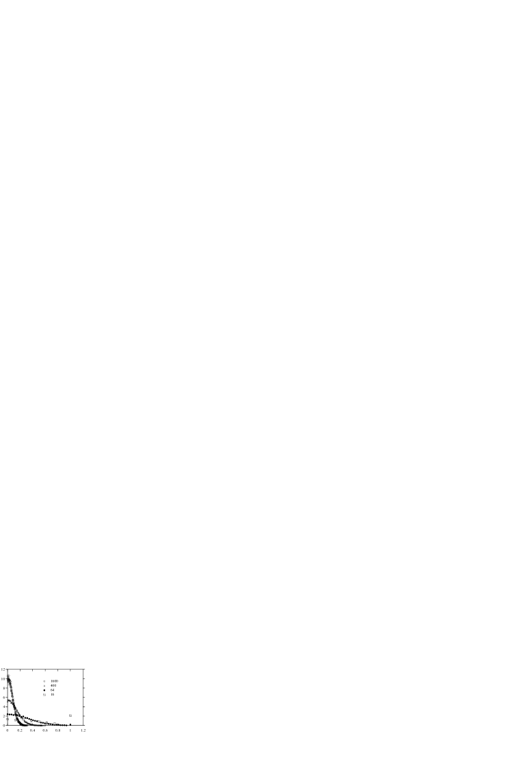
Figure 3: The function $P(q)$ for different values of $N$ ($N=16,64,400,1600$) in the case of the sequential algorithm.

These results are in good agreement with older studies [16, 17]. The surprise come from the study of the distribution function $P(q)$. If we plot the function $P(q)$ for diffeent sizes we do not see anything unexpected (see fig. (3)). The distribution becomes more and more concentrated at $q=0$ when $N\to\infty$.

The crucial point is however how fast the function $P(q)$ decreases with $N$ at fixed $q$. More precisely can define the function

$$f(q)=-\lim_{N\to\infty}{\ln(P_{N}(q))\over N}.$$ (22)

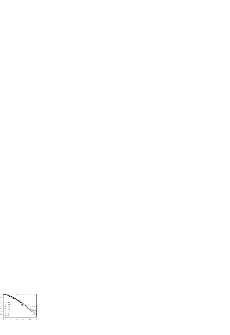
Figure 4: The results obtained with the sequential algorithm for the function $r_{N}(q)$ for $N$ and $q$ ranging from 16 to 1600 and from 0 to 1 respectively.

In the ususal equilibrium SK model the function $f(q)$ is equal to zero in the interval [0-$q_{EA}$] and it is different from zero for $q>q_{EA}$.

The region where $f(q)$ is zero is the essential support of the function $P(q)$. In the region where $f(q)=0$ we can modifying the Hamiltonian by a quantity whose density goes to zero with $N$ (e.g. imposing the appropriate bondary conditions) and we can obtain a system such that the value is $q$.

If the function $P_{N}(q)$ becomes non trivial in the limit $N\to\infty$ the replica symmetry is broken in the usual sence. On the contrary, if the function $P_{N}(q)$ becomes a delta function in the limit $N$ going to infinity, but $f(q)$ is zero in a finite interval, the replica symmetry is broken in a weak sence.

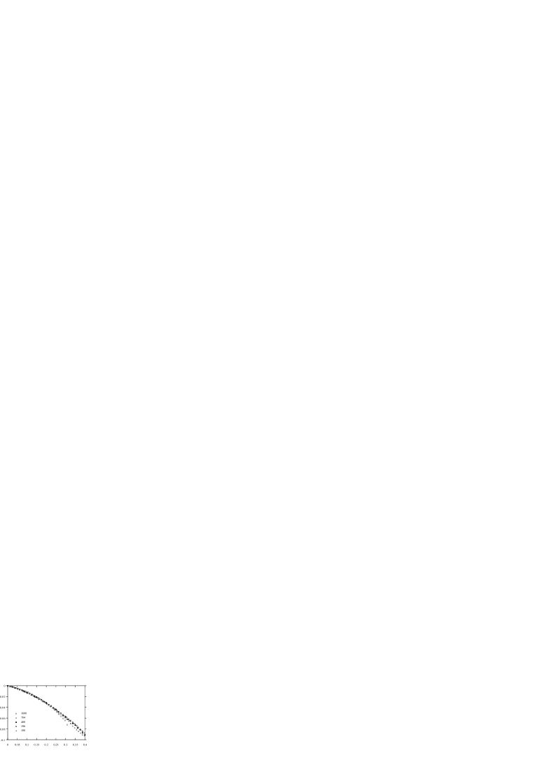
Figure 5: The results obtained with the sequential algorithm for the function $r_{N}(q)$ for $N$ and $q$ ranging from 100 to 1600 and from 0 to .4 respectively.

In fig. (4,5) we plot the quantity

$$r_{N}(q)=N^{-\nu}\ln(\int_{q}^{1}dq^{\prime}P_{N}(q^{\prime})),$$ (23)

with $\nu=2/3$.

This quantity has a very weak dependence on $N$ and it is rather likely that it goes to a non zero value when $N$ goes to infinity in the whole interval 0-1. If we accept this conclusion, we find that $P_{N}(q)$ decreases slower than an exponential for all values of $q$, included $q=1$ and therefore the function $f(q)$ is always zero in the whole interval 0-1. Replica symmetry is thus broken in a weak sence.

If $r_{N}(1)$ has a finite limit, as it is suggested by this data, the probability of finding two times the same solution goes to zero slower than an exponential of $N$, implying that the effective numer of different solutions which can be reached with this method diverges slower that an exponential of $N$.

The other quantity for which we obtain surprising results is the probabily distribution of the fields $h_{i}=\sum_{k}J_{i,k}\sigma_{k}$. The function $P_{N}(h)$ depends weakly on $N$ (the expectation value of $h$ is the energy.

The function $P_{N}(h)$ seem to vanish linearly at $h=0$. In order to show this behaviour in fig. (6) we plot the function

$$\tilde{P}_{N}(h)\equiv{P_{N}(h)\over h+C},$$ (24)

for $N=1600$ where the constant $C$ (which vanishes when $N\to\infty$) has been choosen in such a way to have a smooth behaviour at small $h$. We have found that $C=2N^{-1/2}$ is a good choice. This value of $C$ is natural, indeed the variable $h$ make take values $(n+1/2)C$, with $n$ integer.

Figure 6: The function $\tilde{P}(h))$ in the case of the sequential algorithm.

A linear behaviour of the function $P(h)$ is similar to the one observed at thermal equilibrium at zero temperature, where $P(h)$ is proportional to $h$.

We do not have a simple explanation for such behaviour. The process of minimizing the energy of a given spin has the side effect of decreasing also the energy of the other spins, pushing the distribution of $h$ far from zero. Howevever it is unclear how to transfom this observation in a quantitive prediction.

We have analized also the other dynamics ad we have obtained comparable results. The only remarkable effect that the dependence of the energy on the algorithm is counterintuitive. Indeed the greedy algorithm is the worst (the energy is higher of about .007 than the sequential algorithm) and the reluctant algorithm is much better (the energy -.746 is lower of about .03 than the sequential algorithm). This effect is likely due to the fact that the greedy algorithm is more easily trapped in local minima with high energies and that the slower reluctant algorithm avoids these traps.

5 Conclusions

The probability distribution of the configurations obtained by the zero temperature dynamics have rather peculiar statistical properties. The results obtained are very different from those coming taking a generic solution of the TAP equations with the appropriate energy. The maximum allowed value of $q$ (from the thermodynamic point) is 1, not smaller than $1$ as it would happen for the generic solutions of that energy. Morover the distribution of $h$ is zero at $h$ =0, while there are no reasons that $P(h)$ should be equal to zero at $h=0$ in the case if the generic solution.

It is rather likely the corresponding effective Hamiltonian is not so simple and its statistical properties should be computed using a replica symmetry breaking approach.

It would also interesting to connect the small $h$ behaviour with the power laws observed in the dependence of physical quantities (like the energy of the remanent magnetization) or the number of iterations in the sequential dynamics.

References

- [1]
- [2] J.-P. Bouchaud; J. Phys. France 2 1705, (1992).
- [3] G. Parisi and F. Ritort , J. Phys. A 26 6711 (1993).
- [4] L. F. Cugliandolo, J. Kurchan and F. Ritort, Phys. Rev. B49, 6331 (1994).
- [5] Phys. Rev. Letters 71, 71, (1992).
- [6] L. F. Cugliandolo and J. Kurchan; J. Phys. A27 (1994) 5749; cond-mat 9403040, Phil. Mag. (to be published).
- [7] G. Ferraro, Rome Preprint (1994)
- [8] M. Mézard, G. Parisi and M. A. Virasoro, Spin Glass Theory and Beyond (World Scientific, Singapore 1987).
- [9] G. Parisi, Field Theory, Disorder and Simulations, World Scientific, (Singapore 1992).
- [10] S. Franz and M. Mézard; Off equilibrium glassy dynamics: a simple case, LPTENS 93/39, On mean-field glassy dynamics out of equilibrium, cond-mat 9403004, LPTENS 94/05.
- [11] L. F. Cugliandolo and J.Kurchan; Phys. Rev. Lett. 71, 93 (1993) and references therein.
- [12] E. Marinari, G. Parisi and F. Ritort, Replica Field Theory for Deterministic Models (II): A non-random Spin Glass with glassy Behaviour Hep-th/9406074, summited to J. Phys. A (Math. Gen.).
- [13] A.C.C. Cooley and D. Sherrington, Phys. Rev. E 49 1921 (1994)
- [14] A.C.C. Cooley and S. Franz, cond-mat preprint 9406082.
- [15] G. Parisi, N. Parga and M. A. Virasoro, J. Phys. Lettres 45 (1984) L1063.
- [16] N. Parga, G. Parisi, ICTP preprint (1985), unpublished
- [17] N. Parga J. Phys A 19 51 (1986).
- [18] S. Cabasino, E. Marinari, G. Parisi, P. Paolucci, J. Phys. A (Math. Gen.) 21 (1988) 4201.
- [19] G. Parisi and M. A. Virasoro, J. Phys. 50 (1989) 3317-3329.
- [20] G. Parisi J. Physique 51 (1990) 1595-1606.
- [21] J. Touless, P.W. Anderson and R. G. Palmer Phil. Magaz. 35, 137 (1977).
- [22] L. F. Cugliandolo, J. Kurchan and G. Parisi,Off Equilibrium Dynamics and Aging in Unfrustrated Systems, cond-mat preprint (1994) and references therein.
- [23] L. Cugliandolo Tor Vergata thesis (unpublished) (1994)
- [24] R. Biferale, R. Benzi, G. Parisi, Europhys. Lett. 6, 6 (1992).
- [25] S. Migdal, Phys. Rev E 5, 123 (1992).