Fluctuation Effects and Multiscaling of the Reaction-Diffusion Front for $A+B\rightarrow\emptyset$.

Abstract

We consider the properties of the diffusion controlled reaction $A+B\rightarrow\emptyset$ in the steady state, where fixed currents of $A$ and $B$ particles are maintained at opposite edges of the system. Using renormalisation group methods, we explicitly calculate the asymptotic forms of the reaction front and particle densities as expansions in $(JD^{-1}|x|^{d+1})^{-1}$, where $J$ are the (equal) applied currents, and $D$ the (equal) diffusion constants. For the asymptotic densities of the minority species, we find, in addition to the expected exponential decay, fluctuation induced power law tails, which, for $d<2$, have a universal form $A|x|^{-\omega}$, where $\omega=5+O(\epsilon)$, and $\epsilon=2-d$. A related expansion is derived for the reaction rate profile $R$, where we find the asymptotic power law $R\sim B|x|^{-\omega-2}$. For $d>2$, we find similar power laws with $\omega=d+3$, but with non-universal coefficients. Logarithmic corrections occur in $d=2$. These results imply that, in the time dependent case, with segregated initial conditions, the moments $\int|x|^{q}R(x,t)dx$ fail to satisfy simple scaling for $q>\omega+1$. Finally, it is shown that the fluctuation induced wandering of the position of the reaction front centre may be neglected for large enough systems.

1 Introduction

Since the initial work of Gálfi and Rácz [1], there has been considerable interest in the kinetics of one and two species annihilation, $A+A\rightarrow\emptyset$, and $A+B\rightarrow\emptyset$ [1–17, 23–27]. Most analytic and numerical studies have concentrated on the case of either homogeneous initial conditions, or initially entirely segregated reactants. Ben-Naim and Redner [6] were the first to study the case of a steady state reaction interface, maintained by fixed particle currents imposed at opposite edges of the system. Their equations for the particle densities $a({\bf x},t)$ and $b({\bf x},t)$ were

$${\partial a\over\partial t}=D\nabla^{2}a-\lambda ab$$ (1)

$${\partial b\over\partial t}=D\nabla^{2}b-\lambda ab,$$ (2)

with diffusion constant $D$, reaction rate constant $\lambda$, and with the boundary conditions:

$$J=-D\partial_{x}a|_{x=-L}\quad 0=-D\partial_{x}b|_{x=-L}\quad 0=-D\partial_{x}a|_{x=L}\quad-J=-D\partial_{x}b|_{x=L}.$$ (3)

These equations are asymptotically soluble analytically, giving

$${a\brace b}\sim(J/D)|x|{\theta(-x)\brace\theta(x)}+(const.)\left(J^{2}\over\lambda D\right)^{1/3}\left({\lambda J\over D^{2}}\right)^{-1/12}|x|^{-1/4}e^{-{2\over 3}(\lambda J/D^{2})^{1/2}|x|^{3/2}},$$ (4)

where $\theta(x)$ is the Heaviside step function. The relations $w\sim J^{-1/3}$, where $w$ is the reaction front width, and $c\sim J^{2/3}$, where $c$ is the particle concentration in the reaction zone, are also derived in [6]. However, implicit in their formulation is the ‘mean field’ like assumption, $\langle ab\rangle\propto\langle a\rangle\langle b\rangle$, which will no longer be adequate below the critical dimension, due to fluctuations. Cornell and Droz [12] have given an argument for the upper critical dimension of the system (leading to $d_{c}=2$), as well as performing numerical simulations. On the basis of these, and mean field analysis, they have proposed scaling forms for $a$,$b$ and the reaction front $R$, which are postulated to be valid both above and below the critical dimension in the scaling limit $w\rightarrow\infty$ (or $J\rightarrow 0$):

$$R={J\over w}S\left({x\over w}\right)\qquad a={wJ\over D}A\left({x\over w}\right)\qquad b={wJ\over D}B\left({x\over w}\right).$$ (5)

In other words, the profiles are characterised by a single length scale $w$, which itself is suggested in [12] to vary as $w\sim J^{-1/2}$ in $d=1$, and $w\sim J^{-1/3}$ for $d\geq 2$ in the scaling limit. Cardy and Lee [26] have given RG arguments which support this conclusion. However, we defer further discussion, especially with regard to the presence of multiscaling, until section 6.

In this paper, we present the results of the first renormalisation group calculation for the asymptotic properties of the densities and reaction front in the steady state, which systematically takes into account the effect of fluctuations in the stochastic particle dynamics. Previously, the RG had been used to study the late time behaviour of reactions with homogeneous initial conditions (see [16] and references therein). Our calculational framework will bear considerable similarities with [16]. The basic plan is to map the microscopic dynamics, in the form of a master equation, onto a quantum field theory. This theory is then renormalised (for $d\leq 2$) by the introduction of a renormalised coupling, which is shown to have a stable fixed point of order $\epsilon$. We then group the Feynman diagrams into sets whose sums give a particular order of the renormalised coupling constant. It will be demonstrated that this grouping is given by the number of loops. These diagrams may then be evaluated (asymptotically) and the Callan-Symanzik solution used, to obtain perturbative expansions for the densities and reaction front. Note that for $d>2$ no renormalisation is necessary and the diagrams may be evaluated directly.

We now present our results for the asymptotic forms of the densities and reaction front profile. It will be shown that at zero loops we find a stretched exponential dependence which we include in the following summary, even though we expect its effects to be overwhelmed by leading and subleading power law terms. In addition, for $d<2$, we do not rule out the possibility of logarithms in higher order terms summing to give a modification to the leading power law given below (which results from the straightforward evaluation of the one loop contributions). So we find asymptotically as $|x|\rightarrow\infty$ for $d<2$:

$${\langle a\rangle\brace\langle b\rangle}=(J/D)|x|{\theta(-x)\brace\theta(x)}+A_{1}|x|^{(7-5d)/12}e^{-A_{2}|x|^{(d+1)/2}}+A_{3}|x|^{-5+2\epsilon}+\ldots$$ (6)

$$R=\lambda\langle ab\rangle=A_{4}|x|^{(7d-5)/12}e^{-A_{2}|x|^{(d+1)/2}}+A_{5}|x|^{-7+2\epsilon}+\ldots$$ (7)

where

$$A_{1}=0.3787{(J/D)^{7/12}\over(4\pi\epsilon)^{5/12}}\qquad A_{2}={2\over 3}(4\pi\epsilon)^{1/2}(J/D)^{1/2}\qquad A_{3}={1\over 32\pi^{2}(J/D)\epsilon}$$ (8)

$$A_{4}=0.3787(J/D)^{19/12}{(4\pi\epsilon)^{7/12}\over(9/D)}(d+1)^{2}\qquad A_{5}={(2d+1)(2d+2)\over 32\pi^{2}(J/D^{2})\epsilon};$$ (9)

for $d=2$:

$${\langle a\rangle\brace\langle b\rangle}=(J/D)|x|{\theta(-x)\brace\theta(x)}+B_{1}(\ln|x|)^{5\over 12}|x|^{-{1\over 4}}e^{-B_{2}(\ln|x|)^{-1/2}|x|^{3/2}}+B_{3}|x|^{-5}\ln|x|+\ldots$$ (10)

$$R=B_{4}(\ln|x|)^{-7/12}|x|^{3/4}e^{-B_{2}(\ln|x|)^{-1/2}|x|^{3/2}}+B_{5}|x|^{-7}\ln|x|+\ldots$$ (11)

where

$$B_{1}=0.3787{(J/D)^{7/12}\over(4\pi)^{5/12}}\qquad B_{2}={2\over 3}(4\pi(J/D))^{1/2}\qquad B_{3}={(J/D)^{-1}\over 32\pi^{2}}$$ (12)

$$B_{4}=0.3787(4\pi)^{7/12}D(J/D)^{19/12}\qquad B_{5}={15(J/D)^{-1}\over 16\pi^{2}/D};$$ (13)

and finally, for $d>2$:

$${\langle a\rangle\brace\langle b\rangle}=(J/D)|x|{\theta(-x)\brace\theta(x)}+C_{1}|x|^{-1/4}e^{-C_{2}|x|^{3/2}}+C_{3}|x|^{-d-3}+\ldots$$ (14)

$$R=C_{4}|x|^{3/4}e^{-C_{2}|x|^{3/2}}+C_{5}|x|^{-d-5}+\ldots$$ (15)

where

$$C_{1}=0.3787{(J/D)^{7/12}\over(\lambda/D)^{5/12}}\qquad C_{2}={2\over 3}(\lambda J/D^{2})^{1/2}$$ (16)

$$C_{3}=(\lambda J/D^{2})^{-1}2^{-1-d}\pi^{-(d+1)/2}(d-1)\Gamma\left({d-1\over 2}\right)\qquad C_{4}=0.3787\lambda{(J/D)^{19/12}\over(\lambda/D)^{5/12}}$$ (17)

$$C_{5}=\lambda(\lambda/D)^{-2}(J/D)^{-1}2^{-1-d}\pi^{-(d+1)/2}\Gamma\left({d-1\over 2}\right)(d-1)(d+3)(d+4).$$ (18)

The layout of this paper is as follows. In section 2, the system is defined using a master equation, which is then mapped to a second quantised representation, and then to a field theory. In section 3, we present two related field theories and derive the form of their Green functions. The renormalisation of the theory is also addressed. The calculations for the densities and reaction front are presented in section 4, for $d<d_{c}$, $d=d_{c}$, and $d>d_{c}$. The separate problem of the fluctuations in the position of the centre of the reaction front is presented in section 5. A discussion of these results and comparisons with the available data from simulations are given in section 6, where we also argue for the presence of multiscaling in the system.

2 The Model

We consider a model where A and B particles are moving diffusively on a hypercubic lattice, with lattice constant $l$. There is some probability of mutual annihilation whenever an A and a B particle meet on a lattice site. In addition, particles of type A are added at a constant rate to lattice sites on the hypersurface $x=-L$, and particles of type B are similarly added to sites at $x=L$. In other words, opposing currents of A and B particles are maintained at opposite edges of the system. The two hypersurfaces $x=\pm L$ mark the boundaries of the system beyond which the particles are not permitted to move. The model is defined by a master equation for $P(\{n,m\},t)$, the probability of particle configuration $\{n,m\}$ occurring at time $t$. Here $\{n,m\}=(n_{1},n_{2},\ldots,n_{N},m_{1},m_{2},\ldots,m_{N})$, where $n_{i}$ is the occupation number of the A particles, and $m_{i}$ the occupation number of the B particles, at the $i$th lattice site. The appropriate master equation is

$$\qquad{\partial\over\partial t}P(\{n,m\},t)=$$

$${D\over l^{2}}\sum_{i,e}\{(n_{e}+1)P(\dots n_{i}-1,n_{e}+1,\dots,\{m\},t)-n_{i}P(\{n,m\},t)\}\qquad\qquad$$

$$+{D\over l^{2}}\sum_{i,e}\{(m_{e}+1)P(\{n\},\dots m_{i}-1,m_{e}+1,\dots,t)-m_{i}P(\{n,m\},t)\}$$

$$+\lambda\sum_{i}[(n_{i}+1)(m_{i}+1)P(\dots n_{i}+1,m_{i}+1\dots,t)-n_{i}m_{i}P(\dots n_{i},m_{i}\dots,t)]$$

$$+R\{P(\dots,n_{-L}-1,\{m\},t)-P(\dots,n_{-L},\{m\},t)\}$$

$$+R\{P(\{n\},m_{L}-1\dots,t)-P(\{n\},m_{L}\dots,t)\},$$ (19)

where $i$ is summed over lattice sites, and $e$ is summed over the nearest neighbours of $i$. The first, second, and third lines of the equation describe diffusion of the A and B particles respectively (with equal diffusion constants $D$), whilst the fourth line describes their annihilation within the system (with rate constant $\lambda$). The final four terms are due to the addition of A and B particles at the edges of the system at a rate $R$, corresponding to the maintenance of steady particle currents.

The master equation can be mapped to a second quantised form, following a standard procedure developed by Doi [18] and Peliti [19], and as described by Lee [16]. In brief, in terms of the creation/annihilation operators $a,a^{{\dagger}},b,b^{{\dagger}}$ which are introduced at each lattice site, the time evolution operator for the system is

$$\hat{H}=-{D\over l^{2}}\sum_{i,e}\{a_{i}^{{\dagger}}(a_{e}-a_{i})+b_{i}^{{\dagger}}(b_{e}-b_{i})\}-\lambda\sum_{i}(1-a_{i}^{{\dagger}}b_{i}^{{\dagger}})a_{i}b_{i}-R\{a_{-L}^{{\dagger}}-1+b_{L}^{{\dagger}}-1\}.$$ (20)

This can now be mapped onto a path integral, in which $a,\hat{a},b,\hat{b}$ are replaced by continuous c-number fields, with action (up to a constant)

$$S=\sum_{i}\left(\int_{-\infty}^{t}dt\left\{\hat{a}_{i}\dot{a}_{i}+\hat{b}_{i}\dot{b}_{i}-{D\over l^{2}}\left[\hat{a}_{i}\sum_{e}(a_{e}-a_{i})+\hat{b}_{i}\sum_{e}(b_{e}-b_{i})\right]\right.\right.$$

$$\left.\left.\qquad\qquad-\lambda(1-\hat{a}_{i}\hat{b}_{i})a_{i}b_{i}\right\}-a_{i}(t)-b_{i}(t)\right),$$ (21)

where $a_{i}(t)$ and $b_{i}(t)$ are due to the projection state (see [16]), provided that

$$R={J\over l}={D\over l^{2}}(a_{o}-a_{-L})\qquad 0={D\over l^{2}}(b_{o}-b_{-L})$$ (22)

at $-L$, and

$$R={J\over l}={D\over l^{2}}(b_{o}-b_{L})\qquad 0={D\over l^{2}}(a_{o}-a_{L})$$ (23)

at $+L$. Here the sites $-L$, $L$ are at the edges of the system, with site $o$ being immediately outside $L$ or $-L$. Taking the continuum limit of this action, we arrive at

$$S[\hat{a},a,\hat{b},b,t]=\int\left(dxd^{d-1}y\int_{-\infty}^{t}dt\left\{\hat{a}(\partial_{t}-D\nabla^{2})a+\hat{b}(\partial_{t}-D\nabla^{2})b\right.\right.$$

$$\left.\left.\qquad\qquad\qquad\qquad\qquad\qquad\qquad-\lambda_{0}(1-\hat{a}\hat{b})ab\right\}-a(t)-b(t)\right).$$ (24)

subject to the conditions

$$-J=-D\partial_{x}b\qquad 0=-D\partial_{x}a$$ (25)

at $+L$, and

$$J=-D\partial_{x}a\qquad 0=-D\partial_{x}b$$ (26)

at $-L$. Here $y$ are the coordinates for directions perpendicular to the applied currents. These conditions may be made explicit in the action by including a pair of delta functions:

$$S=\int\left(dxd^{d-1}y\int_{-\infty}^{t}dt\left\{\hat{a}(\partial_{t}-D\nabla^{2})a+\hat{b}(\partial_{t}-D\nabla^{2})b\right.\right.$$ (27)

$$\left.\left.\qquad\quad-\lambda_{0}(1-\hat{a}\hat{b})ab-\hat{a}J\delta(x+L)-\hat{b}J\delta(x-L)\right\}-a(t)-b(t)\right).$$

If we make the substitutions $\hat{a}=1+\bar{a}$ and $\hat{b}=1+\bar{b}$, then the action becomes (up to a constant)

$$S=\int dxd^{d-1}ydt\left[\bar{a}(\partial_{t}-D\nabla^{2})a+\bar{b}(\partial_{t}-D\nabla^{2})b+\lambda_{0}\bar{a}ab+\lambda_{0}\bar{b}ab\right.$$

$$\left.\qquad\qquad\qquad\qquad+\lambda_{0}\bar{a}\bar{b}ab-\bar{a}J\delta(x+L)-\bar{b}J\delta(x-L)\right].$$ (28)

If we integrate over the $\bar{a}$ and $\bar{b}$ fields, and neglect the $\bar{a}\bar{b}ab$ term, we obtain the classical (mean field) equations

$$(\partial_{t}-D\nabla^{2})a+\lambda_{0}ab-J\delta(x+L)=0$$ (29)

$$(\partial_{t}-D\nabla^{2})b+\lambda_{0}ab-J\delta(x-L)=0.$$ (30)

On the further conditions that no particle annihilation occurs at the edges of the system, and that $\nabla a=0$ and $\nabla b=0$ outside, integrating the first equation from $-L-\epsilon$ to $-L+\epsilon$ and the second from $L-\epsilon$ to $L+\epsilon$ in the limit $\epsilon\rightarrow 0$ gives the required boundary conditions.

As the diffusion constant exhibits no singular behaviour in the renormalisation of the theory, it is convenient to absorb it into a rescaling of time, as in [16]. Defining $\bar{t}=Dt$, $\bar{\lambda}=\lambda_{0}D^{-1}$, and $\bar{J}=JD^{-1}$, and introducing the fields $\phi={1\over 2}(a+b)$ and $\psi={1\over 2}(a-b)$, we have

$$S=\int dxd^{d-1}yd\bar{t}\left[2\bar{\phi}(\partial_{\bar{t}}-\nabla^{2})\phi+2\bar{\psi}(\partial_{\bar{t}}-\nabla^{2})\psi+2\bar{\lambda}\bar{\phi}(\phi^{2}-\psi^{2})+\right.$$ (31)

$$\left.\bar{\lambda}(\bar{\phi}^{2}-\bar{\psi}^{2})(\phi^{2}-\psi^{2})-\bar{J}\bar{\phi}[\delta(x+L)+\delta(x-L)]-\bar{J}\bar{\psi}[\delta(x+L)-\delta(x-L)]\right].$$

Consequently, the new classical equations of the steady state are

$$\partial_{x}^{2}\psi_{c}+{1\over 2}\bar{J}[\delta(x+L)-\delta(x-L)]=0$$ (32)

$$\partial_{x}^{2}\phi_{c}-\bar{\lambda}(\phi_{c}^{2}-\psi_{c}^{2})+{1\over 2}\bar{J}[\delta(x+L)+\delta(x-L)]=0.$$ (33)

The appropriate solution for $\psi_{c}$ is just $-(\bar{J}/2)x$ (for $|x|\leq L$), whilst substituting $\phi_{c}=(\bar{J}/2)|x|+u$ into the second equation gives asymptotically the Airy equation for $u$, as noted in [6]. Asymptotically one finds

$$\phi_{c}={J\over 2D}|x|+0.3787\left({J^{2}\over D\lambda}\right)^{1/3}\left({\lambda J\over D^{2}}\right)^{-1/12}|x|^{-1/4}e^{-(2/3)(\lambda JD^{-2})^{1/2}|x|^{3/2}}+\ldots,$$ (34)

where the constant was determined numerically.

So far the quartic term in the action has been neglected, with the result that the simple mean field results have been recovered. However, we can take into account the non-classical term by including Gaussian noise in the equations for $\phi$ and $\psi$, leading to equations which are exact. This modification can be derived by replacing the quartic piece in the action by a noise variable, integrating over the noise distribution, and demonstrating that this recovers the original term. Observing that

$$\int_{-\infty}^{\infty}d\eta_{\phi}e^{\bar{\phi}\eta_{\phi}}e^{-\eta_{\phi}^{2}/[4\bar{\lambda}(\phi^{2}-\psi^{2})]}\sim e^{\bar{\lambda}\bar{\phi}^{2}(\phi^{2}-\psi^{2})},$$ (35)

and

$$\int_{-\infty}^{\infty}d\eta_{\psi}e^{\bar{\psi}\eta_{\psi}}e^{-\eta_{\psi}^{2}/[4\bar{\lambda}(\phi^{2}-\psi^{2})]}\sim e^{-\bar{\lambda}\bar{\psi}^{2}(\phi^{2}-\psi^{2})},$$ (36)

where $\eta_{\phi}$ and $\eta_{\psi}$ are complex Gaussian noise variables with an appropriate phase, we see that the steady state equations may be written as

$$\partial_{x}^{2}\psi+{1\over 2}\bar{J}[\delta(x+L)-\delta(x-L)]+\eta_{\psi}=0$$ (37)

$$\partial_{x}^{2}\phi-\bar{\lambda}(\phi^{2}-\psi^{2})+{1\over 2}\bar{J}[\delta(x+L)+\delta(x-L)]+\eta_{\phi}=0.$$ (38)

Clearly we have lost the simple interpretation of the $a$ and $b$ fields as being the local densities of A and B particles, as now each of the above equations includes a (generally) complex noise term. Nevertheless, we can still interpret $\langle\psi\rangle$ and $\langle\phi\rangle$ as being averaged densities, which also satisfy

$$\partial_{x}^{2}\langle\psi\rangle+{1\over 2}\bar{J}[\delta(x+L)-\delta(x-L)]=0$$ (39)

$$\partial_{x}^{2}\langle\phi\rangle-\bar{\lambda}\langle\phi^{2}-\psi^{2}\rangle+{1\over 2}\bar{J}[\delta(x+L)+\delta(x-L)]=0.$$ (40)

The second equation will be used later on to relate a perturbation expansion for $\langle\phi\rangle$ to one for $\langle\phi^{2}-\psi^{2}\rangle$.

Finally, we give the natural canonical dimensions for the various quantities appearing in the action, noting that the coupling becomes dimensionless at the postulated value of the critical dimension [12]:

$$[\bar{t}]=k^{-2}\qquad[a,b]=k^{d}\qquad[\bar{a},\bar{b}]=k^{0}\qquad[\bar{\lambda}]=k^{2-d}\qquad[\bar{J}]=k^{d+1}.$$ (41)

3 Field Theory Formulations

In what follows it will be convenient to develop two parallel field theories - one given by the action already described in (31), and another to be described below, formed by writing $\phi=\phi_{c}+\phi_{1}$ and $\psi=\psi_{c}+\psi_{1}$. In particular, whilst the second theory is more useful for calculations, the cancellation of divergences after renormalisation, and the identification of leading terms in an expansion in powers of the coupling constant, are easier to see in the first theory.

3.1 Propagators and Vertices

The propagators for the first of the two theories described above (which we shall call Field Theory I) are (from (31))

$$G_{\phi\bar{\phi}}(k,\bar{t})=G_{\psi\bar{\psi}}(k,\bar{t})={1\over 2}e^{-k^{2}\bar{t}},$$ (42)

in $(k,\bar{t})$ space. In $(k,s)$ space, where a Laplace transform of time has been performed, we have

$$G_{\phi\bar{\phi}}(k,s)=G_{\psi\bar{\psi}}(k,s)={1/2\over k^{2}+s}.$$ (43)

The vertices are shown in figure 1, where the $\phi$ propagators are represented by solid lines, and $\psi$ propagators by dotted lines.

For Field Theory II, we split the $\phi$ and $\psi$ fields into their classical and non-classical components, which leads to a modified action

$$S=\int dxd^{d-1}yd\bar{t}\left\{2\bar{\phi}(\partial_{\bar{t}}-\nabla^{2}+2\bar{\lambda}\phi_{c})\phi_{1}+2\bar{\psi}(\partial_{\bar{t}}-\nabla^{2})\psi_{1}\right.$$ (44)

$$\left.+2\bar{\lambda}\bar{\phi}(\phi_{1}^{2}-\psi_{1}^{2}-2\psi_{c}\psi_{1})+\bar{\lambda}(\bar{\phi}^{2}-\bar{\psi}^{2})(\phi_{c}^{2}+2\phi_{c}\phi_{1}+\phi_{1}^{2}-\psi_{c}^{2}-2\psi_{c}\psi_{1}-\psi_{1}^{2})\right\},$$

where the classical equations have been used to simplify its form somewhat. We can now substitute for the exact value of $\psi_{c}=-(\bar{J}/2)x$ and for the functional form of the $\phi_{c}$ field (from (33))

$$\phi_{c}=(\bar{J}^{2}/\bar{\lambda})^{1/3}f[(\bar{\lambda}\bar{J})^{1/3}x].$$ (45)

If we also make the rescaling in the action of

$$\tilde{x}=(\bar{\lambda}\bar{J})^{1/3}x\quad\tilde{y}=(\bar{\lambda}\bar{J})^{1/3}y\quad\tilde{t}=(\bar{\lambda}\bar{J})^{2/3}\bar{t},$$ (46)

then it is transformed to

$$S=\int d\tilde{x}d^{d-1}\tilde{y}d\tilde{t}(\bar{\lambda}\bar{J})^{-{d\over 3}}\left[2\bar{\phi}(\partial_{\tilde{t}}-\tilde{\nabla}^{2}+2f(\tilde{x}))\phi_{1}+2\bar{\psi}(\partial_{\tilde{t}}-\tilde{\nabla}^{2})\psi_{1}\right.$$

$$\left.\qquad\qquad\qquad+2(\bar{\lambda}/\bar{J}^{2})^{1/3}\bar{\phi}(\phi_{1}^{2}-\psi_{1}^{2})+2\bar{\phi}\tilde{x}\psi_{1}\right.$$

$$\left.+(\bar{\phi}^{2}-\bar{\psi}^{2})\left((\bar{J}^{2}/\bar{\lambda})^{1\over 3}h(\tilde{x})+2f(\tilde{x})\phi_{1}+\tilde{x}\psi_{1}+(\bar{\lambda}/\bar{J}^{2})^{1\over 3}(\phi_{1}^{2}-\psi_{1}^{2})\right)\right],$$ (47)

where

$$h(\tilde{x})=[f(\tilde{x})]^{2}-{1\over 4}\tilde{x}^{2},$$ (48)

which is essentially just the classical profile of the reaction front. The form of the propagators is now

$$G_{\phi_{1}\bar{\phi}}={1\over 2}(\bar{\lambda}\bar{J})^{d/3}G(\tilde{x},\tilde{x}^{\prime},{\bf\tilde{y},\tilde{y}^{\prime}},\tilde{t}),$$ (49)

where

$$[\partial_{\tilde{t}}-\tilde{\nabla}^{2}+2f(\tilde{x})]G(\tilde{x},\tilde{x}^{\prime},{\bf\tilde{y},\tilde{y}^{\prime}},\tilde{t})=\delta(\tilde{x}-\tilde{x}^{\prime})\delta({\bf\tilde{y}-\tilde{y}^{\prime}})\delta(\tilde{t}-\tilde{t}^{\prime});$$ (50)

and

$$G_{\psi_{1}\bar{\psi}}(\tilde{k},\tilde{s})={1\over 2}(\bar{\lambda}\bar{J})^{d/3}{1\over\tilde{k}^{2}+\tilde{s}},$$ (51)

in $(\tilde{k},\tilde{s})$ space, or

$$G_{\psi_{1}\bar{\psi}}(\tilde{x}-\tilde{x}^{\prime},\tilde{k}_{\perp},\tilde{s})=(\bar{\lambda}\bar{J})^{d/3}{e^{-(\tilde{k}_{\perp}^{2}+\tilde{s})^{1/2}|\tilde{x}-\tilde{x}^{\prime}|}\over 4(\tilde{k}_{\perp}^{2}+\tilde{s})^{1/2}},$$ (52)

in $(\tilde{x},\tilde{k}_{\perp},\tilde{s})$ space, where the perpendicular directions are defined to be those perpendicular to the applied currents. Unfortunately the equation for $G$ (50) is too hard to solve exactly, as we do not have an analytic form for $\phi_{c}$. Consequently we must rely on the approximation $f(\tilde{x})\sim{1\over 2}|\tilde{x}|$, valid at large $|\tilde{x}|$, in order to make the equation tractable. If we also Laplace transform time, and Fourier transform to momentum space for spatial dimensions perpendicular to the applied currents, then we obtain

$$\left(\tilde{s}+\tilde{k}_{\perp}^{2}-\partial_{\tilde{x}}^{2}+|\tilde{x}|\right)G(\tilde{x},\tilde{x}^{\prime},\tilde{k}_{\perp},\tilde{s})=\delta(\tilde{x}-\tilde{x}^{\prime}).$$ (53)

This has the solution (for $\tilde{x}^{\prime}>0$, and accurate for large $|\tilde{x}|$ i.e. when $|x|\gg(\bar{\lambda}\bar{J})^{-1/3}$):

$$G(\tilde{x},\tilde{x}^{\prime},\tilde{k}_{\perp},\tilde{s})=\cases{\alpha Ai[-\tilde{x}+\tilde{k}_{\perp}^{2}+\tilde{s}]&when $\tilde{x}\leq 0$\cr\beta Ai[\tilde{x}+\tilde{k}_{\perp}^{2}+\tilde{s}]+\gamma Bi[\tilde{x}+\tilde{k}_{\perp}^{2}+\tilde{s}]&when $0\leq\tilde{x}\leq\tilde{x}^{\prime}$\cr\delta Ai[\tilde{x}+\tilde{k}_{\perp}^{2}+\tilde{s}]&when $\tilde{x}\geq\tilde{x}^{\prime}$.\cr}$$ (54)

Considering the boundary conditions at $\tilde{x}^{\prime}$ (continuity in $G$ and a discontinuity in its derivative), we have

$$\beta Ai(\tilde{x}^{\prime}+\tilde{k}_{\perp}^{2}+\tilde{s})+\gamma Bi(\tilde{x}^{\prime}+\tilde{k}_{\perp}^{2}+\tilde{s})=\delta Ai(\tilde{x}^{\prime}+\tilde{k}_{\perp}^{2}+\tilde{s})$$ (55)

$$\beta Ai^{\prime}(\tilde{x}^{\prime}+\tilde{k}_{\perp}^{2}+\tilde{s})+\gamma Bi^{\prime}(\tilde{x}^{\prime}+\tilde{k}_{\perp}^{2}+\tilde{s})-\delta Ai^{\prime}(\tilde{x}^{\prime}+\tilde{k}_{\perp}^{2}+\tilde{s})=1.$$ (56)

These equations can be solved for $\gamma$ with the result that $\gamma=\pi Ai(\tilde{x}^{\prime}+\tilde{k}_{\perp}^{2}+\tilde{s})$. The final boundary condition ($G\rightarrow 0$ as $\tilde{x}\rightarrow-\infty$) will (in principle) give a further relation between $\beta$ and $\gamma$, as well as specifying $\alpha$. But to use this condition we need to know the behaviour of $G$ in regions near $0$, where our asymptotic approximation breaks down. Consequently we must rely on numerical solutions, which reveal that for our purposes we may neglect the $\beta Ai$ term in (55). Solving for $\delta$, we obtain:

$$G(\tilde{x},\tilde{x}^{\prime},\tilde{k}_{\perp}^{2},\tilde{s})=\cases{\pi Ai(\tilde{x}^{\prime}+\tilde{k}_{\perp}^{2}+\tilde{s})Bi(\tilde{x}+\tilde{k}_{\perp}^{2}+\tilde{s})&for $0\ll\tilde{x}\leq\tilde{x}^{\prime}$\cr\pi Bi(\tilde{x}^{\prime}+\tilde{k}_{\perp}^{2}+\tilde{s})Ai(\tilde{x}+\tilde{k}_{\perp}^{2}+\tilde{s})&for $\tilde{x}\geq\tilde{x}^{\prime}\gg 0$.}$$ (57)

We can now use the asymptotic form of the Airy function [20] to simplify these expressions further:

$$Ai(z)\sim{1\over 2\sqrt{\pi}}z^{-1/4}e^{-(2/3)z^{3/2}},\qquad Bi(z)\sim{1\over\sqrt{\pi}}z^{-1/4}e^{(2/3)z^{3/2}}.$$ (58)

Hence, for $0\ll\tilde{x}<\tilde{x}^{\prime}$,

$$G={1\over 2}(\tilde{x}^{\prime}+\tilde{k}_{\perp}^{2}+\tilde{s})^{-1/4}(\tilde{x}+\tilde{k}_{\perp}^{2}+\tilde{s})^{-1/4}e^{-(2/3)[(\tilde{x}^{\prime}+\tilde{k}_{\perp}^{2}+\tilde{s})^{3/2}-(\tilde{x}+\tilde{k}_{\perp}^{2}+\tilde{s})^{3/2}]},$$ (59)

with a similar expression for $\tilde{x}>\tilde{x}^{\prime}\gg 0$. For $\tilde{x}\approx\tilde{x}^{\prime}\gg 0$, we may expand the terms inside the exponential, to obtain

$$G_{\phi_{1}\bar{\phi}}(\tilde{x},\tilde{x}^{\prime},\tilde{k}_{\perp},\tilde{s})={1\over 4}(\bar{\lambda}\bar{J})^{d/3}(\tilde{x}+\tilde{k}_{\perp}^{2}+\tilde{s})^{-1/2}e^{-(\tilde{x}+\tilde{k}_{\perp}^{2}+\tilde{s})^{1/2}|\tilde{x}-\tilde{x}^{\prime}|}.$$ (60)

The important point to notice here is that for $\tilde{x}$ sufficiently close to $\tilde{x}^{\prime}$, the Green function decays only as a power law.

Finally, we note that each occurrence of a propagator is associated with a factor of $(\bar{\lambda}\bar{J})^{d/3}$. If we also extract a factor of $(\bar{\lambda}\bar{J})^{-(d+2)/3}$ from each vertex, then we can use the vertices shown in figure 2, provided we multiply any given diagram by a factor of

$$(\bar{\lambda}\bar{J})^{{1\over 3}pd-{v\over 3}(d+2)},$$ (61)

where $p$ is the number of propagators and $v$ is the number of vertices. Again, in figure 2, $\phi$ propagators are solid lines and $\psi$ propagators are dotted lines. Note the simple form of the vertices (h) to (m).

3.2 Renormalisation

The renormalisation of the theory proceeds in a similar vein to that described in [16] - our field theory differs only in the nature of the boundary conditions. Again the only renormalisation required is coupling constant renormalisation, as the set of vertices for Field Theory I allows no diagrams which dress the propagator. Hence we have no field renormalisation and the bare propagators are the full propagators for the theory.

3.2.1 Renormalisation of the Coupling

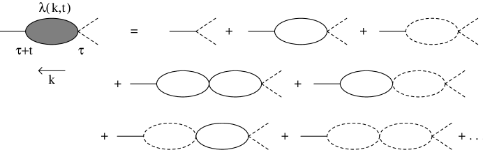
Figure 3: The sum of diagrams contributing to the primitively divergent vertex function $\lambda(k,t)$.

The temporally extended vertex function for $A+B\rightarrow\emptyset$ is given by the sum of diagrams shown in figure 3. This sum may be calculated exactly, as done in [17] (remembering extra factors of two resulting from the presence of two different types of propagator):

$$\bar{\lambda}(k,s)={\bar{\lambda}\over 1+{1\over 2}\bar{\lambda}B_{2}\Gamma(\epsilon/2)(s+{1\over 2}k^{2})^{-\epsilon/2}},$$ (62)

where $B_{2}=2/(8\pi)^{d/2}$, and $\epsilon=2-d$. However, as we are now in the time independent state, we take $s=0$, leading to

$$\bar{\lambda}(k)={\bar{\lambda}\over 1+{1\over 2}\bar{\lambda}B_{2}\Gamma(\epsilon/2)2^{\epsilon/2}k^{-\epsilon}}.$$ (63)

The vertex function can now be used to define the renormalised coupling, with $k=\kappa$ as the normalisation point (differing from [16]). So we have

$$g_{R}=\kappa^{-\epsilon}\bar{\lambda}(k)|_{k=\kappa}\qquad g_{0}=\kappa^{-\epsilon}\bar{\lambda},$$ (64)

for the dimensionless renormalised and bare couplings respectively. The $\beta$ function is defined by

$$\beta(g_{R})\equiv\kappa{\partial\over\partial\kappa}g_{R}=-\epsilon g_{R}+{1\over 2}\epsilon g_{R}^{2}B_{2}\Gamma(\epsilon/2)2^{\epsilon/2},$$ (65)

and we have a fixed point $\beta(g_{R}^{\ast})=0$ when

$$g_{R}^{\ast}=\{2^{-d/2}B_{2}\Gamma(\epsilon/2)\}^{-1}.$$ (66)

The fixed point is of order $\epsilon$. Finally, the expansion of $g_{0}$ in powers $g_{R}$ remains, as in [16]:

$$g_{0}=g_{R}+{g_{R}^{2}\over g_{R}^{\ast}}+\dots\quad$$ (67)

3.2.2 Callan-Symanzik Equation

We now write down the renormalisation group equation for $\langle\phi_{1}\rangle_{R}$ (the renormalised value of $\langle\phi_{1}\rangle$), expressing its lack of dependence on the normalisation scale:

$$\left(\kappa{\partial\over\partial\kappa}+\beta(g_{R}){\partial\over\partial g_{R}}\right)\langle\phi_{1}\rangle_{R}(x,g_{R},\kappa,\bar{J})=0.$$ (68)

In addition, dimensional analysis implies

$$\left(\kappa{\partial\over\partial\kappa}-x{\partial\over\partial x}+(d+1)\bar{J}{\partial\over\partial\bar{J}}\right)\langle\phi_{1}\rangle_{R}(x,g_{R},\kappa,\bar{J})=d\langle\phi_{1}\rangle_{R}(x,g_{R},\kappa,\bar{J}).$$ (69)

Eliminating the terms involving $\kappa$, we have

$$\left(x{\partial\over\partial x}-(d+1)\bar{J}{\partial\over\partial\bar{J}}+\beta(g_{R}){\partial\over\partial g_{R}}+d\right)\langle\phi_{1}\rangle_{R}(x,g_{R},\kappa,\bar{J})=0.$$ (70)

This can be solved by the method of characteristics, with solution

$$\langle\phi_{1}\rangle_{R}(x,g_{R},\kappa,\bar{J})=(\kappa x)^{-d}\langle\phi_{1}\rangle_{R}(\kappa^{-1},\tilde{g}_{R}(\kappa^{-1}),\kappa,\tilde{\bar{J}}(\kappa^{-1})),$$ (71)

and associated characteristics

$$x{\partial\tilde{g}_{R}\over\partial x}=\beta(\tilde{g}_{R})\qquad\tilde{g}_{R}(x)=g_{R}$$ (72)

$$x{\partial\tilde{\bar{J}}\over\partial x}=-(d+1)\tilde{\bar{J}}\qquad\tilde{\bar{J}}(x)=\bar{J}.$$ (73)

These equations have the exact solutions:

$$\tilde{\bar{J}}(x^{\prime})=\left({x\over x^{\prime}}\right)^{d+1}\bar{J}$$ (74)

$$\tilde{g}_{R}(x^{\prime})=g_{R}^{\ast}\left(1+{g_{R}^{\ast}-g_{R}\over g_{R}\left({x\over x^{\prime}}\right)^{\epsilon}}\right)^{-1},$$ (75)

where in the large $|x|$ limit $\tilde{g}_{R}\rightarrow g_{R}^{\ast}$.

We can make use of the mechanics developed above by first calculating an expansion in powers of $g_{0}$, which can be converted into an expansion in powers of $g_{R}$ via (67). Provided that the expansion is non-singular in $\epsilon$, we can relate the $g_{R}$ expansion to an $\epsilon$ expansion using (71), where for large $|x|$ we can take $\tilde{g}_{R}\rightarrow g_{R}^{\ast}$.

3.2.3 Tree Diagrams

At this point we need to identify the leading terms in an expansion in powers of $g_{0}$ - something which can be done in a very similar fashion to [16], using Field Theory I. For the calculation of $\langle\phi\rangle$, tree diagrams are of order $g_{0}^{i}\bar{J}^{1+i}$, for integer $i$. Diagrams with $j$ loops will be of order $g_{0}^{i}\bar{J}^{1+i-j}$. As the addition of loops makes the power of $g_{0}$ higher relative to the power of $\bar{J}$, we see that the number of loops will give an indicator of the order of the diagram.

We are now in a position to develop two tree level quantities - namely the classical density and the classical response function. Diagrammatically, we represent the classical densities by wavy lines and the classical response functions by thick lines. The tree level density $\langle\phi\rangle$ is given by the sum of all tree diagrams which end with a $G_{\phi\bar{\phi}}$ propagator, as shown in figure 4(b). This is equivalent to the mean field equation, as may be seen by acting on both sides of the graphical equation by the inverse Green function $2(\partial_{\bar{t}}-\nabla^{2})$. Similarly, acting on the much simpler tree level diagram for $\langle\psi\rangle$ (figure 4(a)) with the inverse Green function gives its classical equation.

We now define the three response functions for the theory:

$$\langle\psi(x,-k_{\perp},-s)\bar{\psi}(x^{\prime},k_{\perp},s)\rangle^{(1)}\qquad\langle\phi(x,-k_{\perp},-s)\bar{\phi}(x^{\prime},k_{\perp},s)\rangle^{(1)}$$

$$\qquad\qquad\qquad\langle\phi(x,-k_{\perp},-s)\bar{\psi}(x^{\prime},k_{\perp},s)\rangle^{(1)},$$ (76)

where the superscript ‘$1$’ indicates that they are defined in Field Theory I. Their diagrammatic sums are shown in figure 5. The first one: $\langle\psi(x,-k_{\perp},-s)\bar{\psi}(x^{\prime},k_{\perp},s)\rangle^{(1)}$ is simply the propagator $G_{\psi_{1}\bar{\psi}}^{(2)}$, where the superscript ‘$2$’ indicates that it belongs to the second field theory. It is also easy to show that the second response function $\langle\phi(x,-k_{\perp},-s)\bar{\phi}(x^{\prime},k_{\perp},s)\rangle^{(1)}$ is equivalent to the propagator $G_{\phi_{1}\bar{\phi}}^{(2)}$. To do this, we rearrange the unrescaled equation for $G_{\phi_{1}\bar{\phi}}^{(2)}$:

$$2(s+k_{\perp}^{2}-\partial_{x}^{2})G_{\phi_{1}\bar{\phi}}^{(2)}(x,x^{\prime},k_{\perp},s)=-4\bar{\lambda}\phi_{c}(x)G_{\phi_{1}\bar{\phi}}^{(2)}(x,x^{\prime},k_{\perp},s)+\delta(x-x^{\prime}).$$ (77)

Including a delta function integration in the first term on the right hand side, and acting on both sides with the inverse Green function, we obtain

$$G_{\phi_{1}\bar{\phi}}^{(2)}(x,x^{\prime},k_{\perp},s)=G_{\phi\bar{\phi}}^{(1)}-4\bar{\lambda}\int G_{\phi\bar{\phi}}^{(1)}(x,x_{1},k_{\perp},s)\phi_{c}(x_{1})G_{\phi_{1}\bar{\phi}}^{(2)}(x_{1},x^{\prime},k_{\perp},s)dx_{1},$$ (78)

where $G_{\phi\bar{\phi}}^{(1)}$ is the $\phi$ propagator for the first field theory. Iteration now generates the appropriate tree level expansion for $\langle\phi(x,-k_{\perp},-s)\bar{\phi}(x^{\prime},k_{\perp},s)\rangle^{(1)}$, and we have $G_{\phi_{1}\bar{\phi}}^{(2)}=\langle\phi\bar{\phi}\rangle^{(1)}$. The remaining response function $\langle\phi\bar{\psi}\rangle^{(1)}$ is, as would be expected, equivalent in the second field theory to the two point vertex sandwiched between a $\phi$ propagator and a $\psi$ propagator.

4 Density and Reaction Front Calculations

We first note that we cannot draw diagrams which terminate with a $\psi_{1}$ propagator in Field Theory II. Consequently, we conclude that $\langle\psi_{1}\rangle=0$, and hence that $\langle\psi\rangle=\psi_{c}$. This also follows from averaging equation (37). We now turn to the asymptotic evaluation of $\langle\phi\rangle$. Inserting the classical (tree level) solution (34) into the Callan-Symanzik solution (71), and making the leading order replacements $\bar{\lambda}\rightarrow g_{R}\kappa^{\epsilon}$, and for large $|x|$, $\tilde{g}_{R}\rightarrow g_{R}^{\ast}$, we obtain

$$\langle\phi\rangle={1\over 2}\bar{J}|x|+0.3787{\bar{J}^{7/12}\over{g_{R}^{\ast}}^{5/12}}|x|^{(7-5d)/12}e^{-(2/3){g_{R}^{\ast}}^{1/2}\bar{J}^{1/2}|x|^{(d+1)/2}}+\dots$$ (79)

If we use the explicit value of $g_{R}^{\ast}$ from (66), then

$$\langle\phi\rangle={1\over 2}\bar{J}|x|+0.3787{\bar{J}^{7/12}\over(4\pi\epsilon)^{5/12}}|x|^{(7-5d)/12}e^{-(2/3)(4\pi\epsilon)^{1/2}\bar{J}^{1/2}|x|^{(d+1)/2}}+\ldots$$ (80)

So the tree level expression consists of the expected linear term, which must be present if the boundary conditions are to be satisfied, together with a stretched exponential component.

4.1 One Loop Contributions

According to our earlier arguments we expect the next order contributions to $\langle\phi\rangle$ (in Field Theory I) to contain one loop embedded somewhere in the tree diagram. The diagrams corresponding to this prescription are shown in figure 6. However, we have shown that we may translate these diagrams into Field Theory II by replacing response functions by propagators. This is convenient as we have analytic expressions for the Green functions in the second field theory (at least asymptotically), and so performing calculations becomes easier. The equivalent diagrams for Field Theory II are shown in figure 7. Notice that the density lines present in the diagrams for Field Theory I have been absorbed into the vertices for Field Theory II, where a factor of $\phi_{c}^{2}-\psi_{c}^{2}$ is present at the source vertex.

We begin by calculating the loop contained in the third diagram of figure 7 (whilst not including its leftmost vertex). At this level of approximation, we replace the source (the incoming classical density lines at the rightmost vertex in Field Theory I) by a delta function at the origin, with a weight equal to the area under the classical reaction front; in other words:

$$\phi_{c}^{2}-\psi_{c}^{2}\rightarrow\left(\int(\phi_{c}^{2}-\psi_{c}^{2})dx^{\prime}\right)\delta(x).$$ (81)

This will be valid provided $\langle\phi\rangle$ decays much more slowly than the classical reaction front - an assumption that will be shown to be justified a posteriori. By integrating the classical equations, we also have the relation

$$\bar{\lambda}\int(\phi_{c}^{2}-\psi_{c}^{2})dx^{\prime}=\bar{\lambda}^{1/3}\bar{J}^{4/3}\int h[(\bar{\lambda}\bar{J})^{1/3}x^{\prime}]dx^{\prime}=\bar{J},$$ (82)

which is simply saying that, classically, the number of particles entering the system is the same as the number being annihilated at the reaction front. This relationship is also true non-classically, if we average over the noise. After we have performed the rescaling $\tilde{x}^{\prime}=(\bar{\lambda}\bar{J})^{1/3}x^{\prime}$, this becomes

$$\int h(\tilde{x}^{\prime})d\tilde{x}^{\prime}=1.$$ (83)

So the vertex factor at the source becomes:

$$\bar{\lambda}^{1/3}\bar{J}^{4/3}h(\tilde{x})\rightarrow\bar{\lambda}^{1/3}\bar{J}^{4/3}\left(\int h(\tilde{x}^{\prime})d\tilde{x}^{\prime}\right)\delta(\tilde{x})=\bar{\lambda}^{1/3}\bar{J}^{4/3}\delta(\tilde{x}).$$ (84)

Hence the loop is given by the integral

$$2\bar{\lambda}^{-1/3}\bar{J}^{2/3}(\bar{\lambda}\bar{J})^{d/3}\int{e^{-(\tilde{k}_{\perp}^{2}+i\tilde{s})^{1/2}|\tilde{x}_{1}^{\prime\prime}|}\over 4(\tilde{k}_{\perp}^{2}+i\tilde{s})^{1/2}}{e^{-(\tilde{k}_{\perp}^{2}-i\tilde{s})^{1/2}|\tilde{x}_{2}^{\prime\prime}|}\over 4(\tilde{k}_{\perp}^{2}-i\tilde{s})^{1/2}}{e^{-(\tilde{x}^{\prime}+\tilde{k}_{\perp}^{2}+i\tilde{s})^{1/2}|\tilde{x}^{\prime}-\tilde{x}_{1}^{\prime\prime}|}\over 4(\tilde{x}^{\prime}+\tilde{k}_{\perp}^{2}+i\tilde{s})^{1/2}}$$

$$\qquad\qquad\qquad\qquad\qquad{e^{-(\tilde{x}^{\prime}+\tilde{k}_{\perp}^{2}-i\tilde{s})^{1/2}|\tilde{x}^{\prime}-\tilde{x}_{2}^{\prime\prime}|}\over 4(\tilde{x}^{\prime}+\tilde{k}_{\perp}^{2}-i\tilde{s})^{1/2}}(2\tilde{x}_{1}^{\prime\prime})(2\tilde{x}_{2}^{\prime\prime})d\tilde{x}_{1}^{\prime\prime}d\tilde{x}_{2}^{\prime\prime}{d^{d-1}\tilde{k}_{\perp}d\tilde{s}\over(2\pi)^{d}},$$ (85)

where the prefactor of ‘$2$’ counts the number of possible diagram configurations, and the $s$ integration is along the real axis. In the integral we have used the form of the propagator for the $\phi$ field valid for $\tilde{x}_{1}^{\prime\prime},\tilde{x}_{2}^{\prime\prime},\tilde{x}^{\prime}\gg 0$, and $\tilde{x}_{1}^{\prime\prime},\tilde{x}_{2}^{\prime\prime}\approx\tilde{x}^{\prime}$, the region from which we expect the dominant contribution (as here the $\phi$ propagator falls off only as a power law). The $\tilde{x}_{1}^{\prime\prime}$ and $\tilde{x}_{2}^{\prime\prime}$ integrations are elementary, giving

$$2\bar{\lambda}^{-1/3}\bar{J}^{2/3}(\bar{\lambda}\bar{J})^{d/3}{1\over 16}\int e^{-(\tilde{k}_{\perp}^{2}+i\tilde{s})^{1/2}\tilde{x}^{\prime}}e^{-(\tilde{k}_{\perp}^{2}-i\tilde{s})^{1/2}\tilde{x}^{\prime}}\left[(\tilde{k}_{\perp}^{2}+i\tilde{s})^{-1/2}-{2\over\tilde{x}^{\prime 2}}\right]$$

$$\qquad\qquad\qquad\qquad\qquad\qquad\left[(\tilde{k}_{\perp}^{2}-i\tilde{s})^{-1/2}-{2\over\tilde{x}^{\prime 2}}\right]{d^{d-1}\tilde{k}_{\perp}d\tilde{s}\over(2\pi)^{d}}.$$ (86)

However, we notice that the leading $\tilde{x}^{\prime}$ part of the integral is in fact a divergent power law. Furthermore, this divergence cannot be cancelled by the renormalisation of the theory, as any such cancellation would have to arise from coupling constant renormalisation at the tree level (using (67)). As the renormalised tree level result is still an exponential, cancellation with a power law cannot occur. Consequently, we must find another mechanism for the removal of the divergence, and this is provided by its cancellation with the divergent loop shown in figure 7b. Turning now to the next to leading $\tilde{x}^{\prime}$ term in the above integral, we have

$$-\bar{\lambda}^{-1/3}\bar{J}^{2/3}(\bar{\lambda}\bar{J})^{d/3}{1\over 4\tilde{x}^{\prime 2}}\int e^{-(\tilde{k}_{\perp}^{2}+i\tilde{s})^{1/2}\tilde{x}^{\prime}}e^{-(\tilde{k}_{\perp}^{2}-i\tilde{s})^{1/2}\tilde{x}^{\prime}}$$

$$\qquad\qquad\left[{1\over(\tilde{k}_{\perp}^{2}+i\tilde{s})^{1/2}}+{1\over(\tilde{k}_{\perp}^{2}-i\tilde{s})^{1/2}}\right]{d^{d-1}\tilde{k}_{\perp}d\tilde{s}\over(2\pi)^{d}}.$$ (87)

This can be rewritten as

$$\bar{\lambda}^{-1/3}\bar{J}^{2/3}(\bar{\lambda}\bar{J})^{d/3}{2\over\tilde{x}^{\prime 2}}{\partial\over\partial\tilde{x}^{\prime}}\int{2e^{-(\tilde{k}_{\perp}^{2}+i\tilde{s})^{1/2}\tilde{x}^{\prime}-(\tilde{k}_{\perp}^{2}-i\tilde{s})^{1/2}\tilde{x}^{\prime}}\over 4(\tilde{k}_{\perp}^{2}+i\tilde{s})^{1/2}4(\tilde{k}_{\perp}^{2}-i\tilde{s})^{1/2}}{d^{d-1}\tilde{k}_{\perp}d\tilde{s}\over(2\pi)^{d}},$$ (88)

i.e. a constant times the derivative of the $\psi$ propagator loop integral. Rewriting the $\psi$ propagators entirely in momentum space, and performing a contour integration for $\tilde{s}$, we end up with

$$\bar{\lambda}^{-1/3}\bar{J}^{2/3}(\bar{\lambda}\bar{J})^{d/3}{1\over\tilde{x}^{\prime 2}}{\partial\over\partial\tilde{x}^{\prime}}\int{e^{i\tilde{p}\tilde{x}^{\prime}}\over{\bf\tilde{k}}^{2}+(\tilde{p}-{\bf\tilde{k}})^{2}}{d^{d}{\bf\tilde{k}}d\tilde{p}\over(2\pi)^{d+1}}.$$ (89)

This integral may be done exactly using some standard results from [21], with the result

$$\bar{\lambda}^{-1/3}\bar{J}^{2/3}(\bar{\lambda}\bar{J})^{d/3}2^{-1-d}\pi^{-(d+1)/2}(1-d)\Gamma\left({d-1\over 2}\right)\tilde{x}^{\prime-d-2}.$$ (90)

To evaluate the contribution to $\langle\phi\rangle$ we now need to include the leftmost vertex and propagator:

$$-(\bar{\lambda}\bar{J})^{d/3}2^{-2-d}\pi^{-(d+1)/2}(1-d)\Gamma\left({d-1\over 2}\right)\int\tilde{x}^{\prime-d-2}\tilde{x}^{-1/2}e^{-\tilde{x}^{1/2}|\tilde{x}-\tilde{x}^{\prime}|}d\tilde{x}^{\prime},$$ (91)

giving the leading order result

$$-(\bar{\lambda}\bar{J})^{-1}2^{-1-d}\pi^{-(d+1)/2}(1-d)\Gamma\left({d-1\over 2}\right)x^{-d-3}.$$ (92)

We may now insert this into the Callan-Symanzik solution (71), and use the results for the running current/coupling (74)/(75), and for the coupling fixed point (66). This leads to the 1 loop density correction

$${x^{-2d-1}\over 32\pi^{2}\bar{J}\epsilon},$$ (93)

which justifies the use of the delta function approximation for the source. The one remaining diagram in figure 7 consists entirely of $\phi$ propagators, and so asymptotically we expect an exponential dependence which we neglect in comparison with the power law. So to this level of accuracy, we have

$$\langle\phi\rangle={1\over 2}\bar{J}|x|+0.3787{\bar{J}^{7/12}\over(4\pi\epsilon)^{5/12}}|x|^{(7-5d)/12}e^{-{2\over 3}(4\pi\epsilon)^{1/2}\bar{J}^{1/2}|x|^{(d+1)/2}}+{|x|^{-2d-1}\over 32\pi^{2}\bar{J}\epsilon}+\ldots$$ (94)

Using the relation (40) it is also straightforward to calculate the form of the reaction front profile:

$$R=\lambda\langle\phi^{2}-\psi^{2}\rangle=0.3787\bar{J}^{19\over 12}{(4\pi\epsilon)^{7/12}\over 9/D}(d+1)^{2}|x|^{(7d-5)/12}e^{-{2\over 3}(4\pi\epsilon)^{1/2}\bar{J}^{1/2}|x|^{(d+1)/2}}$$

$$\qquad\qquad\qquad\qquad\qquad+{(2d+1)(2d+2)|x|^{-2d-3}\over 32\pi^{2}\epsilon\bar{J}/D}+\ldots,$$ (95)

where only the leading terms generated by the differentiation of each of the component parts of (94) have been retained.

Finally, we consider the cancellation of divergences at 1 loop which, as we mentioned earlier, can most easily be seen in the formalism of Field Theory I. We expect divergent contributions from the 1 loop diagrams a,b,c and d in figure 6, in the limit where the position of the loop’s left vertex tends towards that of the right vertex. In this limit, where no insertions are possible into the response functions, it is appropriate to replace the loop of $\phi$ response functions with one of $\psi$ response functions. Evaluating this loop gives the result $1/2g_{R}^{\ast}$, and the diagrams become as shown in figure 8. However, if we consider the corrections to the tree level due to subleading terms in $g_{0}(g_{R})$ (from (67)), we have the same diagrams but with opposite signs, which exactly cancel the 1 loop divergences.

4.1.1 Two Loops

Whilst we have not calculated in full the contributions to the density from the two loop diagrams, a remark concerning their general nature, and of the nature of our perturbation expansion, is in order. A sample of these two loop diagrams is shown in figure 9.

The easiest diagrams to evaluate are the first and second of those in figure 9, for which it is easy to check that they have the form

$$\sim{|x|^{-4d-3}\bar{J}^{-3}\over\epsilon^{2}}\sim\epsilon^{-1/2}|x|^{-d}[\bar{J}|x|^{d+1}\epsilon^{1/2}]^{-3}.$$ (96)

Hence the perturbative expansion for the power law contributions to $\langle\phi\rangle$ would appear to have the form:

$$\langle\phi\rangle\sim\epsilon^{-{1\over 2}}|x|^{-d}[\bar{J}|x|^{d+1}\epsilon^{1/2}]+\epsilon^{-{1\over 2}}|x|^{-d}[\bar{J}|x|^{d+1}\epsilon^{1/2}]^{-1}+\epsilon^{-{1\over 2}}|x|^{-d}[\bar{J}|x|^{d+1}\epsilon^{1/2}]^{-3}+\dots$$ (97)

Consequently, we see that the condition for our field theory to be valid is that the dimensionless parameter $\bar{J}|x|^{d+1}$ be $\gg 1$. It should also be noted that subleading power laws from the loop integrals will be smaller than their leading term by factors of $(\bar{J}|x|^{d+1})^{-1/3}$.

4.2 $d\geq 2$

At the upper critical dimension for the system, in this case $d=2$, we expect logarithmic corrections to the $d>2$ results, owing to the presence of the marginally irrelevant parameter $\bar{\lambda}$. The Callan-Symanzik solution (71) is still valid, although with a different coupling, which we calculate by taking $\epsilon\rightarrow 0$ in (65). This gives the running coupling

$$\tilde{g}_{R}(\kappa^{-1})={g_{R}\over 1+{g_{R}\over 4\pi}\ln(\kappa x)}.$$ (98)

The behaviour of the running current is as previously calculated. Using the asymptotic form $\tilde{g}_{R}\sim 4\pi/\ln(\kappa x)$, we obtain

$$\langle\phi\rangle={1\over 2}\bar{J}|x|+0.3787\bar{J}^{7\over 12}\left({\ln|x|\over 4\pi}\right)^{5\over 12}|x|^{-{1\over 4}}e^{-{2\over 3}(4\pi\bar{J})^{1/2}(\ln|x|)^{-1/2}|x|^{3/2}}+{|x|^{-5}\ln|x|\over 32\pi^{2}\bar{J}}+\ldots,$$ (99)

where higher order corrections will be only $O[(\ln|x|)^{-1}]$ smaller, so the asymptotic regime will be accordingly hard to reach. Finally, for the reaction front, we have

$$R=0.3787D{(4\pi)^{7/12}\bar{J}^{19/12}\over(\ln|x|)^{7/12}}|x|^{3/4}e^{-{2\over 3}(4\pi\bar{J})^{1/2}(\ln|x|)^{-1/2}|x|^{3/2}}+{15D\bar{J}^{-1}|x|^{-7}\ln|x|\over 16\pi^{2}}+\ldots$$ (100)

For dimensions higher than the critical dimension, the expressions from the evaluation of the Feynman diagrams are used directly without being inserted into the Callan-Symanzik solution. This gives us the results, valid for $d>2$, and in the regime $(J^{2}\lambda/D^{3})|x|^{d+4}\gg 1$:

$$\langle\phi\rangle={1\over 2}\bar{J}|x|+0.3787{\bar{J}^{7/12}\over\bar{\lambda}^{5/12}}|x|^{-1/4}e^{-{2\over 3}(\bar{\lambda}\bar{J})^{1/2}|x|^{3/2}}$$

$$\qquad\qquad-(\bar{\lambda}\bar{J})^{-1}2^{-1-d}\pi^{-(d+1)/2}(1-d)\Gamma\left({d-1\over 2}\right)|x|^{-d-3}+\ldots$$ (101)

and

$$R=0.3787\bar{J}^{19/12}\bar{\lambda}^{7/12}D|x|^{3/4}e^{-{2\over 3}(\bar{\lambda}\bar{J})^{1/2}|x|^{3/2}}$$ (102)

$$-D\bar{\lambda}^{-1}\bar{J}^{-1}2^{-1-d}\pi^{-(d+1)/2}\Gamma\left({d-1\over 2}\right)(1-d)(d+3)(d+4)|x|^{-d-5}+\ldots$$

5 Interface Fluctuations

We now turn to the related problem of the nature of fluctuations in position of the reaction front. This is similar to the question of the fluctuations of an interface in the dynamical Ising Model, as described by the time dependent Landau-Ginzburg (TDLG) equation with noise (for example in model A - see [22]). This equation may be mapped to a path integral for the field $\Phi$, with the introduction of response fields $\tilde{\Phi}$, using the Martin-Siggia-Rose formalism:

$$\int{\cal D}\Phi{\cal D}\tilde{\Phi}e^{-\int dxd^{d-1}ydt[\tilde{\Phi}\{\dot{\Phi}+\Gamma(\nabla^{2}\Phi+V^{\prime}(\Phi))\}+{1\over 2}\Gamma\tilde{\Phi}^{2}]},$$ (103)

where the last term in the action results from averaging over the noise. Solving the TDLG equation in the absence of noise gives us the classical profile $\Phi_{c}$, and on physical grounds we expect the full functional form of $\Phi$ to be $\Phi_{c}(x-f(y,t))\approx\Phi_{c}(x)-f(y,t)\Phi^{\prime}_{c}(x)$. The idea now is to substitute this into the action and to expand the response fields in terms of some complete set of eigenfunctions $\Psi_{n}(x)$ :

$$\tilde{\Phi}(x,y,t)=\sum_{n}A_{n}\tilde{f}_{n}(y,t)\Psi_{n}(x),$$ (104)

where the $\{A_{n}\}$ are normalising constants. This set is chosen such that when the $x$ dependence is integrated out of the action, it leaves behind an unambiguous equation for $f(y,t)$, obtained by integrating over the new response fields $\tilde{f}(y,t)$ in the path integral. For the Ising case, $f(y,t)$ can be shown to satisfy a noisy diffusion equation, whose solution implies that fluctuations delocalise the interface for $d\leq 3$. A similar result for reaction fronts would have dramatic consequences.

Returning to the reaction-diffusion system, we expect the functional forms for the fields in our geometry to be $\psi(x-f_{1}(y,t))$ and $\phi(x-f_{2}(y,t))$, by analogy with the Ising case. Considering first the situation where we neglect noise in the system, we expand the above functional forms, giving

$$\phi\approx\phi(x)-f_{2}(y,t)\phi^{\prime}(x)\Rightarrow\phi={1\over 2}\bar{J}|x|\mp{1\over 2}\bar{J}f_{2}\qquad(x=\pm L)$$ (105)

$$\psi=\psi(x)-f_{1}(y,t)\psi^{\prime}(x)\Rightarrow\psi=-{1\over 2}\bar{J}x+{1\over 2}\bar{J}f_{1}.$$ (106)

Hence $a=(1/2)\bar{J}(f_{1}-f_{2})$ and $b=\bar{J}x-(1/2)\bar{J}(f_{1}+f_{2})$ at $x=L$, and $a=-\bar{J}x+(1/2)\bar{J}(f_{1}+f_{2})$ and $b=(1/2)\bar{J}(f_{2}-f_{1})$ at $x=-L$. In the absence of noise $a$ and $b$ represent the (positive) particle densities, so we must have $f_{1}=f_{2}$.

However, if we include the noise term then this argument is invalid, and we proceed, as in the Ising case, by inserting the expanded functional forms for $\phi$ and $\psi$ into the action for Field Theory I, giving

$$S=\int dxd^{d-1}ydt[2\bar{\phi}\{\phi_{c}^{\prime}[-\dot{f}_{2}+\nabla_{\perp}^{2}f_{2}]+2\bar{\lambda}\psi_{c}\psi_{c}^{\prime}(f_{1}-f_{2})\}$$

$$\qquad\qquad\qquad\qquad+2\bar{\psi}\{\psi_{c}^{\prime}[-\dot{f}_{1}+\nabla_{\perp}^{2}f_{1}]\}+\bar{\lambda}(\bar{\phi}^{2}-\bar{\psi}^{2})(\phi_{c}^{2}-\psi_{c}^{2})],$$ (107)

where we have made the approximation $\phi\rightarrow\phi_{c}$, and then used the classical equations to simplify the expression. Here $y$ are the coordinates for directions perpendicular to the applied currents. In our case it is now appropriate to Fourier expand the $\bar{\psi}$ and $\bar{\phi}$ fields, i.e.

$$\bar{\psi}=\sum_{n}\zeta_{n}(y,t)\theta_{n}(x)\qquad\qquad\bar{\phi}=\sum_{n}\xi_{n}(y,t)\theta_{n}(x),$$ (108)

where $\theta_{n}=\sin(n\pi x/L)$ for $n>0$, $\theta_{n}=1/2$ for $n=0$, and $\theta_{n}=\cos(n\pi x/L)$ for $n<0$. Inserting this into the noise term and performing the $x$ integration, we have

$$\int\bar{\psi}^{2}(\phi_{c}^{2}-\psi_{c}^{2})dx=\sum_{n,m}\zeta_{n}\zeta_{m}\int_{-L}^{L}\theta_{n}\theta_{m}(\phi_{c}^{2}-\psi_{c}^{2})dx=\sum_{n,m}\zeta_{n}X_{nm}\zeta_{m},$$ (109)

where $X_{nm}$ is a symmetric matrix which we now diagonalise. Using $\hat{\zeta}_{n}=D_{nm}\zeta_{m}$, but such that $\hat{\zeta}_{0}=\zeta_{0}$, we rewrite (109) as

$$\sum_{n,m}\hat{\zeta}_{n}\Lambda_{nm}\hat{\zeta}_{m},$$ (110)

where ${\bf\Lambda}$ is a diagonal, and ${\bf D}$ a diagonalising, matrix. Bearing in mind the symmetries of the classical solutions, we can perform the $x$ integration within the action to arrive at the path integral:

$$\int{\cal D}f_{1}{\cal D}f_{2}\prod_{n}{\cal D}\hat{\zeta}_{n}{\cal D}\xi_{n}\exp\left[-\int d^{d-1}ydt\left\{2\sum_{n>0}\xi_{n}[A_{n}(-\dot{f}_{2}+\nabla_{\perp}^{2}f_{2})\right.\right.$$ (111)

$$\left.\left.+2\bar{\lambda}B_{n}(f_{1}-f_{2})]+\bar{\lambda}\sum_{n,m}\xi_{n}\xi_{m}X_{nm}+2\hat{\zeta}_{0}C_{0}[-\dot{f}_{1}+\nabla_{\perp}^{2}f_{1}]-\bar{\lambda}\sum_{n}\hat{\zeta}_{n}\Lambda_{nn}\hat{\zeta}_{n}\right\}\right],$$

with

$$A_{n}=\int_{-L}^{L}\theta_{n}\phi_{c}^{\prime}dx,\qquad B_{n}=\int_{-L}^{L}\theta_{n}\psi_{c}\psi_{c}^{\prime}dx,\qquad C_{0}=\int_{-L}^{L}\theta_{0}\psi_{c}^{\prime}dx\sim\bar{J}L.$$ (112)

Integrating over $\hat{\zeta}_{0}$ and $f_{1}$ gives the equation

$$-\dot{f}_{1}+\nabla_{\perp}^{2}f_{1}+\eta=0,$$ (113)

where $\eta$ is a (possibly imaginary) noise variable, with a Gaussian distribution:

$$P(\eta)\sim e^{-(\eta^{2}C_{0}^{2}/\bar{\lambda}|\Lambda_{00}|)}.$$ (114)

If we also diagonalise the noise term involving the $\xi$ fields, then the relevant part of the action is transformed to

$$2\sum_{n>0}W_{n}\hat{\xi}_{n}[A_{n}(\dot{g}-\nabla_{\perp}^{2}g-\eta)-2\bar{\lambda}B_{n}g]+\bar{\lambda}\sum_{n}\hat{\xi}_{n}\Lambda_{nn}\hat{\xi}_{n},$$ (115)

where $g=f_{1}-f_{2}$, and the equation for $f_{1}$ (113) has been added into the action. The $\{W_{n}\}$ are coefficients generated by writing $\xi_{n}$ in terms of $\{\hat{\xi}_{m}\}$. Finally, performing the integrations over $\hat{\xi}_{n}$ and $g$, we find equations for $g$ which can only be mutually consistent for different $n$ if $g=0$, or in other words, if $f_{1}=f_{2}=f$. From (109) we see that $\Lambda_{00}\sim\bar{J}\bar{\lambda}^{-1}$, and so

$$-\dot{f}+\nabla_{\perp}^{2}f+\eta=0,$$ (116)

where $\eta$ is a Gaussian noise variable with probability distribution:

$$P(\eta)\sim e^{-(const.)L^{2}\bar{J}\eta^{2}}.$$ (117)

We now proceed to calculate the mean square fluctuation $\langle f^{2}\rangle-\langle f\rangle^{2}$. This can be done in a straightforward manner, solving the noisy diffusion equation satisfied by $f$ using a Green function method. The results are

$$\langle f(y,t)^{2}\rangle-\langle f(y,t)\rangle^{2}\sim\cases{{\Lambda^{d-3}\bar{J}^{-1}\over L_{\parallel}^{2}}&for $d\geq 4$\cr{\ln(L_{\perp}\Lambda)\bar{J}^{-1}\over L_{\parallel}^{2}}&for $d=3$\cr{L_{\perp}\bar{J}^{-1}\over L_{\parallel}^{2}}&for $d=2$,\cr}$$ (118)

where the system has physical dimensions $L_{\parallel}\times L_{\perp}^{d-1}$, and $\Lambda$ is now the large $k$ momentum cut-off. So we expect that interface fluctuations will be unimportant if

$$\langle f^{2}\rangle-\langle f\rangle^{2}\sim\cases{{\Lambda^{d-3}\over L_{\parallel}^{2}JD^{-1}}\ll L_{\parallel}^{2}\qquad\Rightarrow\qquad{L_{\parallel}^{2}(JD^{-1})^{1/2}\over\Lambda^{(d-3)/2}}\gg 1&for $d\geq 4$\cr{\ln(L_{\perp}\Lambda)\over L_{\parallel}^{2}JD^{-1}}\ll L_{\parallel}^{2}\qquad\Rightarrow\qquad{L_{\parallel}^{2}(JD^{-1})^{1/2}\over(\ln(L_{\perp}\Lambda))^{1/2}}\gg 1&for $d=3$\cr{L_{\perp}\over L_{\parallel}^{2}JD^{-1}}\ll L_{\parallel}^{2}\qquad\Rightarrow\qquad{L_{\parallel}^{2}(JD^{-1})^{1/2}\over L_{\perp}^{1/2}}\gg 1&for $d=2$.}$$ (119)

These results can now be applied to the problem of the late time behaviour of an initially homogeneous distribution of $A$ and $B$ particles [23–26], where it has been shown that the reactants segregate asymptotically [23, 26]. We assume here that we can access the quasistatic time dependent regime by simply replacing our currents $J$ by their time dependent analogues (this point is discussed further in the next section). In [26] it is demonstrated that these time dependent inward currents (towards the domain interfaces) scale as $J\sim t^{-(d+2)/4}$, where the domains have a characteristic length scale which grows in time as $t^{1/2}$. So on the basis of our assumption we can insert the appropriate time dependencies into (119), from where it is easily seen that fluctuations are unimportant for large enough $t$, in dimensions where segregation occurs ($d<4$).

6 Discussion

The main results of our earlier calculations are expansions for the asymptotic behaviour of the density and reaction front profiles for dimensions above, below, and equal to the critical dimension. We now compare our analytic results with the available data from recent numerical simulations [3, 7, 12, 14, 15]. Note that in all of these papers except [12], the initial conditions are those of complete particle segregation - so the particle currents at later times are time dependent. The remaining reference [12] contains the results of simulations in the steady state. In principle, the calculations of this paper can be redone for the time dependent case, but simple one loop considerations for $\langle\psi^{2}\rangle$ indicate that the dominant contributions to the integrals originate from large times. At these times the reaction front is formed quasistatically, and so we expect to be able to relate to the steady state case by making the correspondence $J\sim t^{-1/2}$ [15, 26] (but see below for occasions where this breaks down). Data for $d=2$ in the time dependent situation is presented in [3] and [7], although in [3] there is insufficient information to extract the asymptotic behaviour of the reaction front. Further simulations for $d=2$ and also for $d=1,3$ are given in [12], where evidence for (5) - their proposed scaling form of $R$ - is given. The reaction front profile is seen to exhibit good scaling collapse close to its centre for $d=1,2,3$ but again no information is available for the asymptotics addressed in this paper.

Turning now to the $1d$ case, the simulations in [14, 15] were performed using an infinite reaction rate constant, i.e. if two particles of different species either crossed or occupied the same lattice site, they immediately annihilated. With initial conditions of complete particle segregation, this resulted in total separation of the two species at all later times. Consequently, the reaction front profile was determined by the fluctuations in position of a delta function like reaction front. Our results are for finite reaction rates, and are dominated by density fluctuations which propagate out from the reaction front centre to positions far away, a process which cannot occur in the $1d$ simulations mentioned above. We believe this to be the reason for the discrepancy between our analytic calculations and the numerical results. For example, the $1d$ simulations of Cornell produce evidence for a Gaussian reaction front profile, most notably in figure 8 of [15]. In that graph $\log R$ is plotted against $(x/X^{(2)})^{2}$, where $X^{(2)}$ is the width of the reaction product profile $C=\int R(x,t)dt$, as measured by its second spatial moment. The resulting straight line indicates that the Gaussian profile is maintained well into the asymptotic region (i.e. at least as far as $(x/X^{(2)})^{2}\approx 30$) - in exactly the region where, in our model, we would expect our asymptotic expansion to begin to apply.

In addition, controversy still exists over the spatial moments of the reaction front profile - Araujo et al [14] and Cornell [15] disagree over the presence of multiscaling. In fact, our calculations suggest that multiscaling does indeed occur for high enough moments in the time dependent version of our model, starting from completely segregated initial conditions. For the steady state situation, the existence of the asymptotic power laws found above implies that the moments:

$$x^{(q)}=\left({\int_{-\infty}^{\infty}|x|^{q}R(x)dx\over\int_{-\infty}^{\infty}R(x)dx}\right)^{1/q}$$ (120)

do not exist for $q\geq\omega+1$. However, in the time dependent case, these moments must exist due to the presence of a diffusive cutoff at $x_{D}\sim t^{1/2}$ [27]. Therefore, for the calculation of the spatial moments $x^{(q)}$ (for large enough $q$), we cannot relate the steady state case to the time dependent case by simply applying the scaling substitution $J\sim t^{-1/2}$. We can make these remarks more quantitative by performing the calculation of the spatial moments in the time dependent situation. Separate arguments must be applied for $d<2$, when our RG arguments imply that the steady state profile has a scaling form (95); and for $d>2$, when (102) shows that the fluctuation induced power law tails do not scale. For $d<2$, we have:

$$x^{(q)}(t)\sim\left({\int_{-\infty}^{\infty}|x|^{q}t^{-\beta}S\left({x\over t^{\alpha}}\right)F\left({x\over t^{1/2}}\right)dx\over\int_{-\infty}^{\infty}t^{-\beta}S\left({x\over t^{\alpha}}\right)F\left({x\over t^{1/2}}\right)dx}\right)^{1/q},$$ (121)

where $\alpha$ and $\beta$ are defined in the usual way [1, 26]. Here $F(y)$ is a function which provides a cutoff at $y\sim O(1)$, but whose inclusion does not affect the calculation of moments which are finite even in the absence of a cutoff. For $q<\omega+1$, where the $q$th moment of $S$ is finite (even without a cutoff), we can therefore neglect the effects of $F$. However, for $q>\omega+1$, the $q$th moment is infinite without the cutoff, so the integral will now be dominated by the region $(x/t^{1/2})\sim O(1)$, where the asymptotic result $S\sim(x/t^{\alpha})^{-\omega-2}$ may be used. These considerations lead to the result $x^{(q)}(t)\sim t^{\alpha_{q}}$, where (neglecting any logarithmic corrections for $q=\omega+1$):

$$\alpha_{q}=\cases{\alpha&for $q<\omega+1$\cr{1\over 2}+{(\omega+1)(\alpha-1/2)\over q}&for $q>\omega+1$.}$$ (122)

Hence we have a cusp at $q=\omega+1$, above which $\alpha_{q}$ tends towards $1/2$ for large $q$. Note that this value of $1/2$ is specific to a diffusive cutoff of the form $F(x/t^{1/2})$. For $d=2$ we also expect logarithmic corrections to the above power laws.

For $d>2$, we must carry out a slightly different calculation, as although the classical (tree level) reaction front obeys scaling, (102) reveals that the one loop power law correction does not. However, for moments which exist without a cutoff, it turns out that the classical terms still give the dominant contribution in the scaling limit. For these terms we have, in the steady state case:

$$\int_{-\infty}^{\infty}|x|^{q}R_{c}(x,\lambda,J)dx\sim\lambda^{1/3}J^{4/3}\int_{-\infty}^{\infty}|x|^{q}S_{c}[(\lambda J)^{1/3}x]dx\sim\lambda^{-q/3}J^{1-q/3}.$$ (123)

However, for the non-scaling power law we must consider:

$$(\lambda J)^{-1}\int_{(\lambda J^{2})^{-1/(d+4)}}^{\infty}{x^{q}dx\over x^{d+5}}\sim\lambda^{-q/(d+4)}J^{1-2q/(d+4)},$$ (124)

where we have imposed a lower cutoff in the integral, derived from the expansion parameter of the $d>2$ asymptotic series (102). Comparing the $J$ dependence of the two results above, we see that the first of these will dominate in the scaling limit $J\rightarrow 0$. Substituting $J\sim t^{-1/2}$ and normalising, we end up with $\alpha_{q}=\alpha=1/6$, for $q<d+4$. For the higher moments ($q>d+4$) we need to introduce the cutoff function $F$, so the integral will be dominated by the region $(x/t^{1/2})\sim O(1)$, where we can use the asymptotic power law from (102):

$$x^{(q)}\sim{(\lambda t^{-1/2})^{-1}\over t^{-1/2}}\int_{0}^{\infty}dx{x^{q}\over x^{d+5}}F(x/t^{1/2})\sim\lambda^{-1}t^{(q-2-d)/2}.$$ (125)

Consequently, we have the result $x^{(q)}\sim t^{\alpha_{q}}$, where (neglecting logarithmic corrections for $q=d+4$):

$$\alpha_{q}=\cases{{1\over 6}&for $q<d+4$\cr{1\over 2}-{d+2\over 2q}&for $q>d+4$.}$$ (126)

In this case we have a discontinuity at $q=d+4$, a result of the power law term being unimportant for $q<d+4$, but dominant for $q>d+4$. Once again we stress that the limiting behaviour $\alpha_{q}\rightarrow 1/2$ as $q\rightarrow\infty$ is dependent on the diffusive form of the cutoff.

Thus, we predict the existence of multiscaling in the time dependent case in qualitative agreement with Araujo et al, even though we are considering a different model. In general, power law tails in the steady state reaction front profiles should always lead to dynamic multiscaling, whatever their origin. These arguments are similar to those of Cornell et al. [27], who find evidence for multiscaling in the reaction $nA+mB\rightarrow\emptyset$ with $(n,m)\neq(1,1)$. However, in that case the solutions of the mean field rate equations already give power laws, even without the addition of fluctuation effects.

Finally, we conclude that the available simulations are not directly applicable to our calculations of asymptotic power laws and multiscaling. However, if the asymptotics could be reached in a model with a finite reaction rate, our results should be amenable to numerical tests. These might be easiest in $1d$ where the power law tail should be most pronounced.

Acknowledgments.

The authors would like to thank B. Lee for a reading of the manuscript. We also acknowledge financial support from the EPSRC.

Figure 1: Vertices for Field Theory I.

Figure 2: Vertices for Field Theory II. The couplings associated with each of the above diagrams are: (a). $-\bar{\lambda}^{1/3}\bar{J}^{4/3}h(\tilde{x})$  (b). $\bar{\lambda}^{1/3}\bar{J}^{4/3}h(\tilde{x})$  (c). $-2(\bar{\lambda}\bar{J})^{2/3}\tilde{x}$  (d). $(\bar{\lambda}\bar{J})^{2/3}\tilde{x}$  (e). $-(\bar{\lambda}\bar{J})^{2/3}\tilde{x}$  (f). $-2(\bar{\lambda}\bar{J})^{2/3}f(\tilde{x})$  (g). $2(\bar{\lambda}\bar{J})^{2/3}f(\tilde{x})$  (h). $-2\bar{\lambda}$  (i). $2\bar{\lambda}$  (j). $-\bar{\lambda}$  (k). $\bar{\lambda}$  (l). $\bar{\lambda}$  (m). $-\bar{\lambda}$.

Figure 4: Tree level diagrams for (a) $\langle\psi\rangle$, and (b) $\langle\phi\rangle$.

Figure 5: Response functions for Field Theory I: (a) $\langle\psi\bar{\psi}\rangle^{(1)}$, (b) $\langle\phi\bar{\phi}\rangle^{(1)}$, and (c) $\langle\phi\bar{\psi}\rangle^{(1)}$.

Figure 6: One loop diagrams in Field Theory I.

Figure 7: One loop diagrams in Field Theory II.

Figure 8: Divergences at one loop. The factor underneath each diagram is associated with the vertex.

Figure 9: A sample of the two loop diagrams for $\langle\phi_{1}\rangle$.

References

- [1] Gálfi L. and Rácz Z. 1988 Phys. Rev. A 38 3151.
- [2] Koo Y.E., Li L., and Kopelman R. 1990 Mol. Cryst. Liq. Cryst. 183 187.
- [3] Chopard B. and Droz M. 1991 Europhys. Lett. 15 459.
- [4] Cornell S., Droz M., and Chopard B. 1991 Phys. Rev. A 44 4826.
- [5] Araujo M., Havlin S., Larralde H., and Stanley H.E. 1992 Phys. Rev. Lett. 68 1791.
- [6] Ben-Naim E. and Redner S. 1992 J. Phys. A: Math. Gen. 25 L575.
- [7] Larralde H., Araujo M., Havlin S., and Stanley H.E. 1992 Phys. Rev. A 46 855.
- [8] Larralde H., Araujo M., Havlin S., and Stanley H.E. 1992 Phys. Rev. A 46 R6121.
- [9] Cornell S., Droz M., and Chopard B. 1992 Physica 188A 322.
- [10] Taitelbaum H., Koo Y.E., Havlin S., Kopelman R., and Weiss G. 1992 Phys. Rev. A 46 2151.
- [11] Chopard B., Droz M., Karapiperis T., and Rácz Z. 1993 Phys. Rev. E 47 R40.
- [12] Cornell S. and Droz M. 1993 Phys. Rev. Lett. 70 3824.
- [13] Droz M. and Sasvári L. 1993 Phys. Rev. E 48 R2343.
- [14] Araujo M., Larralde H., Havlin S., and Stanley H.E. 1993 Phys. Rev. Lett. 71 3592.
- [15] Cornell S. 1994 Preprint UGVA/DPT 1994/10-857.
- [16] Lee B.P. 1994 J. Phys. A: Math. Gen. 27 2633.
- [17] Lee B.P. 1994 Critical Behaviour in Non-Equilibrium Systems Ph. D. Thesis, University of California, Santa Barbara; Lee B.P. and Cardy J.L. 1994 Preprint OUTP-94-52S.
- [18] Doi M. 1976 J. Phys. A: Math. Gen. 9 1465; 1976 J. Phys. A: Math. Gen. 9 1479.
- [19] Peliti L. 1985 J. Physique 46 1469.
- [20] Abramowitz M. and Stegun I.A. 1965 Handbook of Mathematical Functions (New York: Dover).
- [21] Gradshteyn I.S. and Ryzhik I.M. 1994 Table of Integrals, Series, and Products (San Diego: Academic Press).
- [22] Hohenberg P.C. and Halperin B.I. 1977 Rev. Mod. Phys. 49 435.
- [23] Bramson M. and Lebowitz J.L. 1991 J. Stat. Phys. 65 941.
- [24] Leyvraz F. and Redner S. 1991 Phys. Rev. Lett. 66 2168; 1992 Phys. Rev. A 46 3132.
- [25] Leyvraz F. 1992 J. Phys. A: Math. Gen. 25 3205.
- [26] Lee B.P. and Cardy J.L. 1994 Preprint OUTP-94-33S.
- [27] Cornell S., Koza Z., and Droz M. 1994 Preprint cond-mat/9412044.