Phase Diagrams for Deformable Toroidal and Spherical Surfaces with Intrinsic Orientational Order

Abstract

A theoretical study of toroidal membranes with various degrees of intrinsic orientational order is presented at mean-field level. The study uses a simple Ginzburg-Landau style free energy functional, which gives rise to a rich variety of physics and reveals some unusual ordered states. The system is found to exhibit many different phases with continuous and first order phase transitions, and phenomena including spontaneous symmetry breaking, ground states with nodes and the formation of vortex-antivortex quartets. Transitions between toroidal phases with different configurations of the order parameter and different aspect ratios are plotted as functions of the thermodynamic parameters. Regions of the phase diagrams in which spherical vesicles form are also shown.

I Introduction

The bilayer fluid membranes, which can form spontaneously when molecules with hydrophobic and hydrophilic parts are introduced to water, are a popular topic of research. In theoretical studies of such membranes, it is usual to work on length scales much larger than the molecular size, so that they can be considered as continuous surfaces; two-dimensional curved spaces embedded in Euclidean three-space. Features commonly incorporated into mathematical models of membranes include bending rigidity $\kappa$ (disaffinity for extrinsic curvature), Gaussian curvature modulus $\kappa_{G}$ (disaffinity for intrinsic curvature), spontaneous curvature due to membrane asymmetries, and for closed surfaces, constraints of constant volume, constant area and constant difference in area between the inner and outer layers. In recent years, interest has grown in membranes whose molecules have orientational order within the surface. For instance, a smectic-A liquid crystal membrane, whose molecules have aliphatic tails which point in an average direction normal to the local tangent plane of the membrane, can undergo a continuous phase transition to smectic-C phase, in which the tails tilt. The tilt is described by a two-component vector order parameter within the surface, given by the local thermal average of vectors parallel to the tails, projected onto to local tangent plane. If such a membrane has intrinsic (Gaussian) curvature, its orientational order is frustrated, since a parallel vector field cannot exist in a curved space. Ordering is further frustrated on a closed surface of spherical topology (genus zero), as an intrinsic vector field must have topological defects whose indices sum to the Euler number of the surface; in this case, two. ie. there must be at least two vortices in the order parameter field on a sphere. The order parameter field vanishes at these defects to avoid infinite gradients. The defects are energetically costly but topologically unavoidable. The energetics of a smectic-C, genus zero membrane were studied by MacKintosh and Lubensky in [1]. There are other types of orientational order. Nematic order is similar to vector order except that its order parameter is locally invariant under rotations through $180^{o}$. Hence nematics can form defects of index $\frac{1}{2}$. Hexatic order is locally invariant under rotations through $60^{o}$, as this is the molecular ‘bond’ angle. The notion may be generalized to fluid phases with $n$-atic orientational order being locally invariant under rotations through $\frac{2\pi}{n}$ and forming defects of index $\frac{1}{n}$. If a vector (‘monatic’) is represented by an arrow then we may picture an $n$-atic as an $n$-headed arrow or an $n$-spoked wheel. For a theoretical study of $n$-atic fluid membranes of genus zero, see [2].

In this paper, theoretical findings on $n$-atic fluid membranes of toroidal topology are presented. As the torus has genus one and Euler number zero, it is possible to arrange an intrinsic vector field on a torus without topological defects. (ie. furry tori can be brushed smooth.) Therefore it appears plausible that $n$-atic membranes with large order parameter coupling compared with bending rigidity may energetically favour a toroidal topology to a spherical one. The object of embarking on this research was to confirm or refute this hypothesis. As will be demonstrated, it turns out to be true, although the arrangements of ordering in the toroidal surface are far more diverse than expected.

Throughout this paper, a number of approximations are used. One approximation is the use of mean field theory. That is, no thermal fluctuations are considered. So the configuration adopted by the system is assumed to be that which minimizes its free energy. Also, the lowest Landau level approximation is employed in constructing the order parameter field, as discussed in section VI. The validity of these approximations is investigated in section X. Both of these approximations give rise to apparent phase transitions between separate, clearly defined states of the system, some of which may in fact be blurred by thermal fluctuations and higher Landau levels, to the point where they disappear. It should therefore be understood that, where reference is made to phase transitions, it is in the context of mean field theory and the lowest Landau level approximation. Before studying the thermal physics, it will be necessary to introduce some tensor calculus. This is needed to describe the behaviour of an $n$-atic field living within a two-dimensional curved space, as well as the intrinsic and extrinsic elastic properties of the space (ie. the membrane) itself. In the absence of intrinsic ordering (ie. under the influence of the membrane’s elasticity alone), one might expect the equilibrium shape of a toroidal vesicle to be axisymmetric. However, such a vesicle is only neutrally stable with respect to one particular mode of non-axisymmetric deformation. This Goldstone mode is discussed in section V, in which a further approximation is introduced, limiting the range of vesicle shapes to be explored. In the sections that follow, the ground-state configurations and energies of the order parameter field are calculated for each of these shapes, subject to the lowest Landau level approximation. Although some of these shapes are never energetically favoured, the behaviour of the field living on them is of interest, if only academic. Finally, in section IX, the total free energy (consisting of order-parameter field and membrane elasticity parts) is minimized with respect to vesicle shape, to find the equilibrium configuration of the system as a function of temperature and the other thermodynamic parameters. The result is a set of phase diagrams for various values of $n$, which contain phases of vesicles with different shapes and ordering. The shapes should be experimentally observable, although the intrinsic ordering is most likely not.

II Values of $n$

$n$ is the order of rotational symmetry. As stated earlier, the fluid membrane is locally invariant under rotations through $\frac{2\pi}{n}$, and the $n$-atic field may be represented by a set of $n$-spoked wheels tessellating. Clearly $n$ is integer. Furthermore, it must be one of the set of numbers for which regular $n$-gons tessellate. That is, $n\in\{1,2,3,4,6\}$. These are the values of $n$ which Park et. al. studied in [2]. However, consider a triangular ($n=3$) lattice with long-range orientational, but no positional order; the $n=3$ analogue of a hexatic lattice. Bonds between neighbouring molecules lie at angles which are integer multiples of $\frac{\pi}{3}$. Its symmetry properties in the absence of positional order are therefore indistinguishable from its dual lattice, the hexatic, and it will form defects of index $\frac{1}{6}$, in preference to the more energetically expensive index $\frac{1}{3}$ defects. To convince oneself of this, it might be helpful to attempt to draw a lattice which has $120^{o}$ rotational symmetry, but does not have $60^{o}$ rotational symmetry. This is only possible if one keeps strict account of the positions of the lattice sites and polygons (ie. in the absence of dislocations). The following research is therefore conducted for $n\in\{1,2,4,6\}$.

III Notation

The $2D$ curved surface is embedded in Euclidean $3$-space. If $\sigma$ is a two-dimensional coordinate of a point $P$ on the surface then $R(\sigma)$ is the position vector of $P$ in the embedding space relative to some origin. Coordinate-dependent unit basis vectors $e_{a}$, where $a$ takes the values $1$ and $2$ to label the coordinates, are defined in the directions of $\partial_{a}\mbox{\boldmath$R$}$. A coordinate-invariant metric tensor is defined on the Riemannian $2$-space, with components $g_{ab}=\partial_{a}\mbox{\boldmath$R$}\cdot\partial_{b}\mbox{\boldmath$R$}$, from which the area of the closed surface is calculated:

$${\cal A}=\int d^{2}\mbox{\boldmath$\sigma$}\sqrt{g}$$ (1)

where $g\equiv\det{\underline{\underline{g}}}$. Indices are raised and lowered by the metric and its inverse, $g^{ab}$, in the standard manner. The extrinsic curvature tensor has components $K_{ab}=\mbox{\boldmath$N$}\cdot\partial_{a}\partial_{b}\mbox{\boldmath$R$}$, where $N$ is a unit vector normal to the surface. (N.B. Dot products are evaluated in $\mbox{\open\char 82\relax}^{3}$.) Its trace, $K^{a}_{a}$, is the ‘total curvature’. Readers may be familiar with the mean curvature which is half of this quantity. The intrinsic or Gaussian curvature is given by $K=\det{\underline{\underline{K}}}$.

As an example, the above quantities are calculated for a sphere of radius $R$, using spherical polar coordinates $(\theta,\phi)$. The metric tensor may be represented by a matrix:

$$\underline{\underline{g}}\doteq\left(\begin{array}[]{cc}g_{11}&g_{12}\\ g_{21}&g_{22}\end{array}\right)=R^{2}\left(\begin{array}[]{cc}1&0\\ 0&\mbox{sin}^{2}\theta\end{array}\right),$$

with determinant $g=R^{4}\mbox{sin}^{2}\theta$. Hence the area element for integration is $\sqrt{g}\,d^{2}\mbox{\boldmath$\sigma$}=\sin{\theta}\,d\theta\,d\phi$, which is just the Jacobian for spherical polars. Any continuous, doubly differentiable surface has two principal radii of curvature, $R_{1}$ and $R_{2}$ at each point. These are the radii of curvature of the geodesics passing through that point which have respectively the greatest and least curvature as measured in the Euclidean embedding space. It can be shown [3] that these two geodesics are always perpendicular. If the particular coordinate basis used corresponds to these two perpendicular directions, then the curvature tensor will be diagonal, and given by

$$\underline{\underline{K}}\doteq\left(\begin{array}[]{cc}K_{1}^{1}&K_{1}^{2}\\ K_{2}^{1}&K_{2}^{2}\end{array}\right)=\left(\begin{array}[]{cc}\frac{1}{R_{1}}&0\\ 0&\frac{1}{R_{2}}\end{array}\right).$$

Of course, on a sphere, curvature is constant. Therefore $K_{a}^{b}=-\frac{\delta_{a}^{b}}{R}$ where the sign convention denotes the direction of the normal. However, it should be noted that, without one index raised, the components are not constant:

$$\left(\begin{array}[]{cc}K_{11}&K_{12}\\ K_{21}&K_{22}\end{array}\right)=-R\left(\begin{array}[]{cc}1&0\\ 0&\mbox{sin}^{2}\theta\end{array}\right).$$

Clearly, on a sphere, mean curvature is $-\frac{1}{R}$ and Gaussian curvature is $\frac{1}{R^{2}}$.

Recall that the intrinsic $n$-atic order in the system is orientational, not positional, and that it is locally invariant under rotations through $\frac{2\pi}{n}$. As this orientational order is intrinsic to a 2-dimensional space, in can be represented by a complex order parameter in the following way. Let $\Theta$ be the local angle between $e_{1}$ and the orientation of ordering. For vector order, this orientation is easily defined. For instance, in a smectic-C membrane, it is the direction of a molecule’s aliphatic tail projected onto the local tangent plane of the membrane. However, in a nematic liquid crystal, $\Theta$ may take one of two values for each molecule, depending on which end of the molecule one chooses to measure from. For our purposes, it does not matter which of these two values is assigned to $\Theta$ at each point. For bond-angle orientational order, eg. hexatic, there is an $n$-fold ambiguity in the definition of $\Theta$ but again, it does not matter which of the $n$ orientations is chosen. It is conventional in this case to define $\Theta$ at a given molecule as the angle between the basis vector $e_{1}$ and the line joining that molecule to its nearest neighbour. Having defined $\Theta$, the order parameter is given by

$$\psi(\mbox{\boldmath$\sigma$})=\left<\exp(in\Theta(\mbox{\boldmath$\sigma$}))\right>$$ (2)

where $<>$ denotes a thermal average. Note that $\psi$ has the appropriate rotational invariance, since a rotation of the orientation of ordering through an angle $\chi$ within the surface is represented by a rotation of $\psi$ through $n\chi$ in the Argand plane. Hence rotating the orientation of ordering through $\frac{2\pi}{n}$ corresponds an identity transformation in the complex plane.

IV The Model

The model used is identical to that in [2]. There is zero spontaneous curvature as the bilayers considered are symmetric, and no constraint on bilayer area difference. The vesicle’s volume is also unconstrained since small solvent molecules may diffuse freely in and out, so long as the solvent is very pure; containing no free ions, which would lead to osmotic pressure. The membrane’s area ${\cal A}$ is fixed by the number of constituent molecules. The free energy functional

$$F[\psi(\mbox{\boldmath$\sigma$}),\mbox{\boldmath$R$}(\mbox{\boldmath$\sigma$})]/T=\int d^{2}\mbox{\boldmath$\sigma$}\sqrt{g}\,\left(\,r|\psi|^{2}+\mbox{$\frac{1}{2}$}u|\psi|^{4}+CD^{a}\psi D^{*}_{a}\psi^{*}+\mbox{$\frac{1}{2}$}\kappa(K^{a}_{a})^{2}+\kappa_{G}K\,\right)$$ (3)

closely resembles the Ginzburg-Landau free energy for classical superconductors. For a discussion of how the thermodynamic coefficients relate to real physical and chemical quantities, see for instance [9]. As defined in Eq.(2), the phase of $\psi$ depends on the choice of basis vectors. Hence the derivatives $D_{a}$ in Eq.(3) must be covariant in order for the quantity $D^{a}\psi D^{*}_{a}\psi^{*}$ to be physical. Let the basis vectors be rotated through an angle $-\chi(\mbox{\boldmath$\sigma$})$. Consequently,

$$\begin{array}[]{lclcl}\psi&\rightarrow&\psi^{\prime}&=&\psi e^{in\chi(\mbox{\boldmath$\sigma$})}\\ \partial_{a}&\rightarrow&\partial^{\prime}_{a}&=&\Lambda_{a}^{\>c}\partial_{c}\\ g_{ab}&\rightarrow&g^{\prime}_{ab}&=&\Lambda_{a}^{\>c}\Lambda_{b}^{\>d}g_{cd}\end{array}$$

where $\Lambda_{a}^{\>c}(\mbox{\boldmath$\sigma$})$ are the components of the rotation matrix. Given that $D_{a}=\partial_{a}-inA_{a}$, demanding that $D^{a}\psi D^{*}_{a}\psi^{*}$ is invariant under the gauge transformation implies that the components of $A$ transform like

$$\begin{array}[]{lclcl}A_{a}&\rightarrow&A^{\prime}_{a}&=&\Lambda_{a}^{\>c}(A_{c}+\partial_{c}\alpha)\,.\end{array}$$ (4)

So $A$ undergoes the usual transformation, $\partial_{a}\alpha$, of a vector potential in a gauge-invariant derivative. But, in addition there is a coordinate rotation, $\Lambda_{a}^{\>c}$ since, in this complex number representation, a rotation of the Argand plane is always accompanied by a rotation of the basis vectors. The ‘spin connection’, $A_{a}=\mbox{\boldmath$e$}_{1}\cdot\partial_{a}\mbox{\boldmath$e$}_{2}$ has the appropriate transformation property Eq.(4). On the sphere, $A_{\theta}=0$ and $A_{\phi}=-\cos{\theta}$.

V The Curvature Energy Terms

Above the continuous transition to the disordered phase, $\psi$ vanishes and only the last two terms in the free energy Eq.(3) survive. These constitute the Helfrich Hamiltonian, describing the elastic energy of a constant area membrane.

The intrinsic curvature energy, being proportional to the integral of Gaussian curvature, is a topological invariant, according to the Gauss-Bonnet formula

$$\int K\,d{\cal A}=2\pi\chi$$ (5)

where $\chi$ is the Euler number of the closed surface [4]. For an orientable surface, $\chi=2(1-G)$, where $G$ is the surface’s genus; ie. how many ‘handles’ it has. Hence the intrinsic curvature energy is zero for a torus and $4\pi\kappa_{G}$ for a sphere.

The total curvature energy, $\frac{\kappa}{2}\int(K^{a}_{a})^{2}\,d{\cal A}$, is a conformal invariant [5]. ie. it is invariant under shape changes of the form

$$\mbox{\boldmath$R$}\rightarrow\mbox{\boldmath$R^{\prime}$}=\frac{\frac{\mbox{\boldmath$R$}}{|R|^{2}}+\mbox{\boldmath$\beta$}}{\left|\frac{\mbox{\boldmath$R$}}{|R|^{2}}+\mbox{\boldmath$\beta$}\right|^{2}}$$ (6)

where $\beta$ is a constant vector which parameterizes the conformal transformation [6]. A sphere has total curvature energy $8\pi\kappa$ and its shape is not changed by such a transformation. This is not true for tori. An axisymmetric, circular cross section torus may be deformed by a conformal transformation. As a consequence of the circular cross-section, a component of $\beta$ parallel to the symmetry axis serves only to change the torus’s size. Hence there remains only a one-parameter family of non-trivial conformal transformations. With $\beta$ lying in the symmetry plane, the surface is deformed into a non-axisymmetric torus such as the one in Fig.(1), and as $\beta$ increases in magnitude, the asymmetry increases until, in the limit, the torus becomes a perfect sphere with an infinitesimal handle.

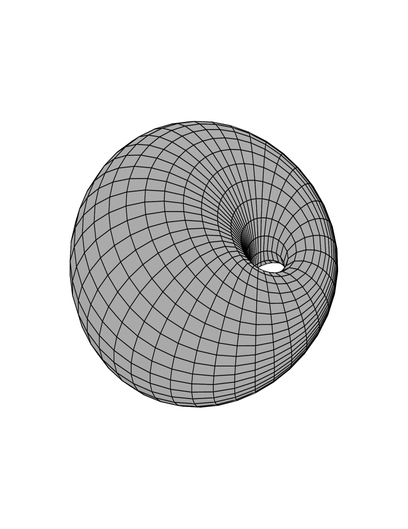
FIG. 1.: The surface produced by a conformal transformation of an axisymmetric, circular cross-section torus.

The handle, although infinitesimal, must contain an intrinsic curvature energy of $-4\pi\kappa_{G}$ and finite total curvature energy. A circular, axisymmetric torus of aspect ratio (ratio of radii of generating circles) $\alpha$ has total curvature energy

$$\frac{\kappa}{2}\int(K^{a}_{a})^{2}\,d{\cal A}=\frac{2\pi^{2}\alpha^{2}\kappa}{\sqrt{\alpha^{2}-1}},$$ (7)

which is a minimum at $\alpha=\sqrt{2}$ , the Clifford torus, and infinite at $\alpha=1$, where the torus becomes self-intersecting. Willmore conjectured [7] that Clifford’s torus and its conformal transformations have the absolute minimum curvature energy of any surface of toroidal topology; a conjecture that is difficult to prove, as the most general toroidal surface cannot easily be parameterized: tori can even be knotted. Accordingly, this paper will not explore the whole of phase space. The discussion will be restricted to axisymmetric, circular cross-section tori and their conformal transformations, with the assumption that these are close to the ground state shapes. To be consistent, the ground-state genus-zero shape is approximated by a sphere: the deviations from sphericity calculated in [2] are not included.

VI The Lowest Landau Level Approximation

The field gradient energy term in Eq.(3) may be re-formulated. Using integration by parts, it is simple to show that, on a closed surface,

$$\int d^{2}\mbox{\boldmath$\sigma$}\sqrt{g}\,g^{ab}D_{a}\psi D^{*}_{b}\psi^{*}=-\int d^{2}\mbox{\boldmath$\sigma$}\psi^{*}D_{a}(\sqrt{g}\,g^{ab}D_{b}\psi).$$ (8)

Let $\phi_{p}$ be eigenfunctions satisfying the Hermitian equation

$$-\frac{D_{a}(\sqrt{g}\,D^{a})\phi_{p}}{\sqrt{g}}=\Lambda\phi_{p}$$ (9)

and the orthonormalization condition

$$\int d^{2}\mbox{\boldmath$\sigma$}\sqrt{g}\,\phi^{*}_{p}\phi_{q}=\frac{\cal A}{4\pi}\delta_{pq}.$$ (10)

These are the Landau levels. $\psi$ may be expanded in this complete set of functions. However, close to the mean-field transition, it is a good approximation to use only the Landau levels with the lowest eigenvalue, $\Lambda_{0}$. As is common in such problems, there is a degenerate set of lowest Landau levels.

$\Lambda$ scales inversely with area. So let us define a scale-invariant eigenvalue $\lambda$, by

$$\Lambda\equiv\frac{4\pi}{\cal A}\lambda.$$ (11)

The free energy becomes

$$F/T=\int\left\{\left(r+\frac{4\pi C\lambda_{0}}{\cal A}\right)|\psi|^{2}+\frac{u}{2}|\psi|^{4}\right\}d{\cal A}+\mbox{curvature energy}$$

where

$$\psi=\sum_{p}a_{p}\phi_{p}$$ (12)

and $a_{p}$ are complex constants. Note that the mean field transition has been lowered from $r=0$ to $r=r_{c}$ where $r_{c}\equiv-\frac{4\pi C\lambda_{0}}{\cal A}$. On an intrinsically flat surface, $\lambda_{0}=0$ but it is finite and positive-definite on a surface with finite Gaussian curvature. So ordering is frustrated by intrinsic curvature.

VII Solution of the Eigenfunction Equation

Eq.(9) may be re-written as the differential equation

$$\left[g^{ab}\right]\partial_{a}\partial_{b}\phi_{p}+\left[(\frac{\partial_{b}-2inA_{b}}{\sqrt{g}})(\sqrt{g}\,g^{ab})\right]\partial_{a}\phi_{p}+\left[\frac{-inD_{a}}{\sqrt{g}}(\sqrt{g}\,g^{ab}A_{b})\right]\psi_{p}=-\frac{4\pi}{\cal A}\lambda\phi_{p}.$$ (13)

This is still general to any surface.

A Sphere

On a sphere, in spherical polar coordinates $(\theta,\phi)$, Eq.(13) becomes

$$\left(\frac{\partial^{2}}{\partial\theta^{2}}+\mbox{cosec}^{2}\theta\frac{\partial^{2}}{\partial\phi^{2}}+\cot\theta\frac{\partial}{\partial\theta}+2in\mbox{cosec}\theta\cot\theta\frac{\partial}{\partial\phi}-n^{2}\cot^{2}\theta\right)\phi_{p}=-\frac{4\pi\lambda}{\cal A}\phi_{p}$$ (14)

which is solved by $\lambda_{0}=n$ and $\phi_{p}$ of the form

$$\phi_{p}\propto\sin^{n+j}\left(\mbox{$\frac{\theta}{2}$}\right)\cos^{n-j}\left(\mbox{$\frac{\theta}{2}$}\right)e^{ij\phi}$$ (15)

where $p$ takes integer values from $-n$ to $n$. These functions form an alternative basis set to that used in [2] and are linear combinations of that set. They are given in [8] in a different gauge. The functions have $2n$ zeros, which are topological defects of index $\frac{1}{n}$. The $(2n+1)$-fold degeneracy reflects the freedom of the defects to lie anywhere on the surface at no energy cost to order $\psi^{2}$.

B Axisymmetric Torus

On tori, $\phi_{p}$ and $\lambda$ depend on $\alpha$ and $\beta$. Consider first the axisymmetric case ($\beta=0$). Let us define coordinates $(\eta,\phi)$. The azimuthal angle is $\phi$, varying around the large generating circle and subtended at the centre. The angle $\eta$ varies around the smaller generating circle and is measured from the symmetry plane, as shown in Fig.(2).

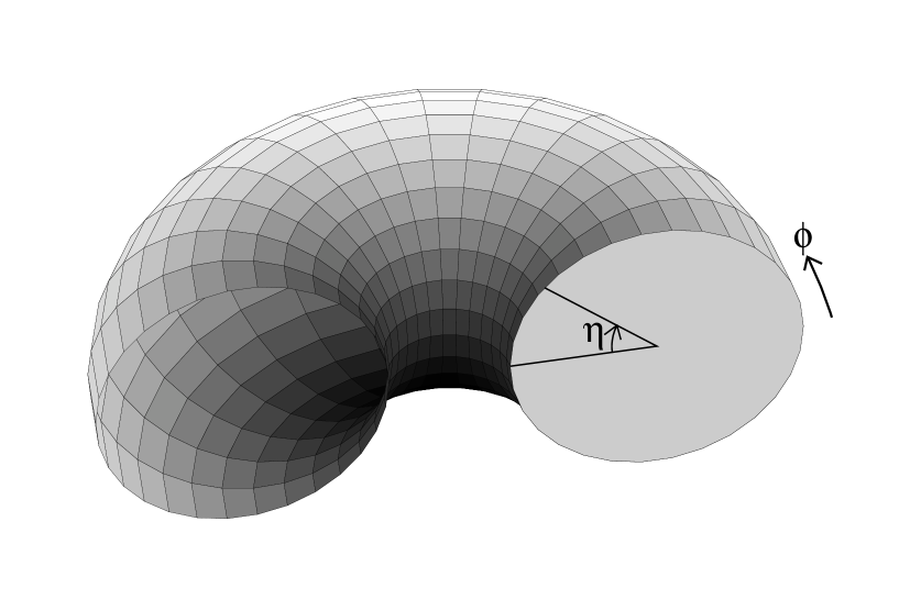
FIG. 2.: The angular coordinates $(\eta,\phi)$ defined on an axisymmetric, circular cross-section torus. For clarity, only half of the torus is shown.

Let the small generating circle have radius $R_{0}$. In this coordinate system, the following quantities are found:

$$g_{ab} \doteq R_{0}^{2}\left(\begin{array}[]{cc}1&0\\ 0&(\alpha-\cos\eta)^{2}\end{array}\right)$$

$$K_{a}^{b} \doteq \frac{1}{R_{0}}\left(\begin{array}[]{cc}-1&0\\ 0&\frac{\cos\eta}{\alpha-\cos\eta}\end{array}\right)$$

$$A_{a} \doteq \left(\begin{array}[]{c}0\\ -\sin\eta\end{array}\right)$$

The Landau level equation Eq.(13) becomes

$$\left[\partial_{\eta}\partial_{\eta}+\frac{\partial_{\phi}\partial_{\phi}}{(\alpha-\cos\eta)^{2}}+\frac{\sin\eta}{\alpha-\cos\eta}\partial_{\eta}+\frac{2in\sin\eta}{(\alpha-\cos\eta)^{2}}\partial_{\phi}-n^{2}\left(\frac{\sin\eta}{\alpha-\cos\eta}\right)^{2}\right]\phi_{p}=\frac{4\pi\lambda}{\cal A}\phi_{p},$$ (19)

which is manifestly invariant under $\eta\rightarrow-\eta$ with complex conjugation, reflecting the up-down mirror symmetry of the torus. Note that changing variable from $\eta$ to $\theta\equiv(\eta-\frac{\pi}{2})$ and setting $\alpha$ to zero re-creates the sphere equation (Eq.(14)).

Eq.(19) has separable variables and is solved by functions of the form

$$\phi_{p}(\eta,\phi)=f_{p}(\eta)e^{ip\phi}$$ (20)

for integer $p$, where

$$\left[\frac{d^{2}}{d\eta^{2}}+\frac{\sin\eta}{(\alpha-\cos\eta)}\frac{d}{d\eta}-\left(\frac{p+n\sin\eta}{\alpha-\cos\eta}\right)^{2}\right]f_{p}=\frac{4\pi\lambda}{\cal A}f_{p}$$ (21)

and $f_{p}$ is real. It is immediately apparent from the form of Eq.(21) that

$$f_{p}(\eta)=f_{-p}(-\eta)$$ (22)

and consequently $\phi_{p}$ and $\phi_{-p}$ are degenerate pairs of states.

The ground-state solutions of Eq.(21) were found numerically for various values of $p$ and $\alpha$, using Rayleigh-Ritz variational method. Trial functions were synthesized from a truncated Fourier series,

$$f_{p}^{\mbox{trial}}=\sum_{\nu=0}^{\nu_{\mbox{max}}}\left(a_{\nu}\cos{\nu\eta}+b_{\nu}\sin{\nu\eta}\right),$$

which has the appropriate periodic boundary conditions. The Fourier coefficients were used as variational parameters to minimize the integral

$$\int_{0}^{2\pi}(\alpha-\cos\eta)f_{p}^{\mbox{trial}}\left[\frac{d^{2}}{d\eta^{2}}+\frac{\sin\eta}{(\alpha-\cos\eta)}\frac{d}{d\eta}-\left(\frac{p+n\sin\eta}{\alpha-\cos\eta}\right)^{2}\right]f_{p}^{\mbox{trial}}\>d\eta$$ (23)

subject to Eq.(10). The minimal value of Eq.(23) is an upper bound on $\lambda_{0}$ , and the corresponding function $f_{p}^{\mbox{trial}}$ is approximately $f_{p}$ . Using a Fourier series truncated after frequency $\nu_{\mbox{max}}$ creates a $(2\nu_{\mbox{max}}+1)$-dimensional parameter space to explore in the numerical minimization. So CPU time increases very rapidly with $\nu_{\mbox{max}}$. A second numerical method was also used, which involved numerically ‘integrating’ Eq.(21) forward in $\eta$ from $\eta_{0}$ to $\eta_{0}+2\pi$ and minimizing the resultant discontinuities in $f_{p}$ and its derivative, with respect to the initial conditions and $\lambda$. This method is more accurate than the Rayleigh-Ritz method but more difficult to use since, depending on the starting conditions, it may find a non-ground-state solution. However, it was useful in establishing the accuracy of the upper bounds. Using $\nu_{\mbox{max}}=7$, $\lambda_{0}$ was found to an accuracy of 0.05% in the worst case.

In Fig.(3), $\lambda(\alpha)$ is plotted for $0\leq p\leq n$, with data points at increments of 0.5 in $\alpha$ and cubic spline interpolation. The states are labelled $n_{p}$. One might have guessed that $n_{0}$ would be the ground state in each case. And indeed, for large aspect ratios, when the torus is almost cylinder-like, the $p=0$ states do have the lowest energy. These states are even functions of $\eta$, being larger at $\eta=\pi$ than at $\eta=0$ where there is more absolute intrinsic curvature, and do not vary with $\phi$. ie. The field does not twist with respect to the coordinate lines as $\phi$ increases. However, for smaller $\alpha$, states with non-zero $p$ are energetically favoured.

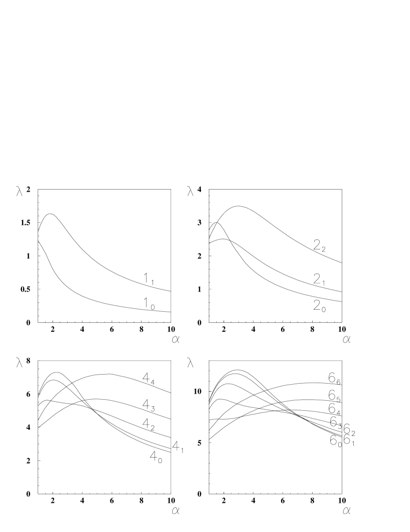
FIG. 3.: Graphs of $\lambda$ against $\alpha$ for axisymmetric, circular cross-section tori. The states are labelled $n_{p}$.

Before explaining the reason for this, it is necessary to describe these states. Fig.(4) depicts a selection of states for $n=2$ on a Clifford torus. The nematic-order field is represented by sets of double-ended lines directed along the orientations of order in the surface of the torus. The length of each line is proportional to $|\psi|$ at that point. Note however that the three-dimensional views of the toroidal surface cause the lines to be foreshortened at oblique angles to the line of sight.

FIG. 4.: Various Landau levels of the $n=2$ (nematic) order-parameter field on a Clifford torus. States are labelled $n_{p}$ and shown in plan view and side view and $\eta$ dependence is given graphically.

Two views are shown of each field on the toroidal surface, as well as a graph of $f(\eta)$. Note that positive $p$ states have a large field on the bottom of the torus and small on the top, and vice versa for negative $p$. This asymmetry becomes more pronounced with increasing $p$, with increasing $n$, and with decreasing $\alpha$. As stated earlier, ordering is frustrated by intrinsic curvature. And the net amount of intrinsic curvature on the torus is constant. But as $\alpha$ decreases, the curvature is redistributed. It becomes more negative around the hole and more positive around the outside of the torus, with the top and bottom remaining fairly flat. So this is where the field prefers to reside and be parallel. Although in Eq.(20) non-zero $p$ states appear to twist with respect to the coordinate basis as $\phi$ increases, the basis itself twists on the top and bottom of the torus as the hole is circled. The two twists cancel. Note that the diagram of the $2_{-2}$ state depicts a field which is as parallel as possible on the top ‘face’ of the torus. Of course, the field on the inner and outer ‘rims’ still contributes to the free energy so, as $\alpha$ increases, the ground-state value of $p$ decreases by a series of ‘transitions’. This is clear in Fig.(3). These should not be regarded as true phase transitions, since the lowest Landau level approximation breaks down completely at these points. As a crossover between eigenvalues is approached, the true state is a mixture of the two states.

It should be emphasized that the tori studied here are true, curved tori, embedded in 3-space. They should not be confused with a flat torus, which is a plane with opposite edges identified, for which the above energetics would not apply. The two have the same topology, but different local geometries.

C Non-Axisymmetric Torus

When $\beta\neq 0$, the Landau level equation (Eq.(13)) becomes much more complicated and its variables are no longer separable. However, Rayleigh-Ritz variational method is again possible, as

$$\lambda_{0}(\alpha,\beta)\leq\int_{{\cal A}=4\pi}\phi^{*}_{\mbox{trial}}D_{a}(\sqrt{g}\,D^{a})\phi_{\mbox{trial}}\,d^{2}\mbox{\boldmath$\sigma$},$$ (24)

but the trial wavefunctions are now complex, periodic functions of two variables. Thus, synthesizing them with a truncated, two-dimensional, complex Fourier series up to frequency $\nu_{\mbox{max}}$ produces an $(8\nu_{\mbox{max}}^{2}+8\nu_{\mbox{max}}+1)$-dimensional space of variational parameters to be numerically explored. Hence ground-state functions of the coordinates with high frequency components cannot viably be found. This is unfortunate since conformally transforming an axisymmetric torus with the coordinate system described above, leaves the coordinates very unevenly distributed over the surface, with most of the interval from $0$ to $2\pi$ in $\eta$ and $\phi$ covering only the small ‘handle’ part of the torus and only a small range covering most of the area. This problem is partly solved by a coordinate transformation $(\eta,\phi)\rightarrow(\rho,\sigma)$ which preserves the metric’s diagonalization, where

$$[1-\beta(\alpha-1)]\tan\frac{\rho}{2} = [1-\beta(\alpha+1)]\tan\frac{\eta}{2}$$

$$\left[1+\beta(\alpha+1)\right]\tan\frac{\sigma}{2} = [1-\beta(\alpha+1)]\tan\frac{\phi}{2}$$

although this still leaves some high frequency components in the distribution of the coordinates on the handle. Using these coordinates, Eq.(24) is very complicated but two special cases are already known:

• When $\beta=0$, the torus is axisymmetric and $\lambda_{0}$ was found by the method in section VII B.

• When $\beta=\frac{1}{R_{0}(\alpha+1)}$ , where $R_{0}$ is the radius of the small generating circle, the torus becomes a sphere with an infinitesimal handle. Hence $\lambda_{0}=n$ and the ground-state function is that of a sphere with all $2n$ zeros at the handle.

Unfortunately, the problem is too computer-intensive to produce any useful results for intermediate values of $\beta$. Using $\nu_{\mbox{max}}=3$ and performing the minimization in a 98-dimensional parameter space took a considerable amount of CPU time per data point. At this level, no states of intermediate $\beta$ were found to have a lower eigenvalue than the known axisymmetric or spherical states. Some local minima were found but these are very likely to be artifacts of the varying reliability of the upper bound, which was high by around 10% for $\beta=0$ and 60% in the spherical limit. More research on this problem is planned. But for the moment, it is necessary to work with the ansatz that:

• A spherical vesicle exists when its total free energy is lower than that of an axisymmetric torus.

• An axisymmetric torus exists when its total free energy is lower than that of a sphere and its field energy alone is lower than that of a sphere.

• A non-axisymmetric torus exists otherwise.

VIII The $\psi^{4}$ term

A Axisymmetric Torus

It was noted earlier that $\phi_{p}$ and $\phi_{-p}$ are degenerate to quadratic order in $\psi$. So, from Eq.(12), $\psi$ is a linear combination of $\phi_{p}$ and $\phi_{-p}$, where $p$ has the ground-state value for the given aspect ratio. The relative proportions of the two states are determined by the $\psi^{4}$ term in Eq.(3). Let

$$\Psi=a_{+}\phi_{p}+a_{-}\phi_{-p}$$

be the function which minimizes $\int|\Psi|^{4}d{\cal A}$ on a surface of area $4\pi$ subject to $|a_{+}|^{2}+|a_{-}|^{2}=1$, and let J be the minimal value of that integral. Then Eq.(3) is minimized by $\psi=a\Psi$ in the regime of the lowest Landau level approximation, where $a$ is real. The gauge invariance and axial symmetry of the problem allow us to choose the phases of both $a_{+}$ and $a_{-}$. Hence $\Psi$ is determined by a minimization with respect to just one parameter.

For some values of $\alpha$ and $p$, it is found that $\Psi=\frac{1}{\sqrt{2}}(a_{+}+a_{-})$. So the ‘top’ and ‘bottom’ states co-exist and, although each is fairly parallel on its own side of the torus, the two do not mesh smoothly where they meet. Consequently, there are $2p$ defects each of index $\frac{1}{n}$ around the torus’s outer ‘rim’ and $2p$ of index $\frac{-1}{n}$ round the inside of the hole: a total of $4p$ defects. Hence as $\alpha$ varies and $p$ jumps between integer values as described above, vortex-antivortex quartets are formed or destroyed. Let these symmetrical states be labelled $n^{S}_{p}$. The $4^{S}_{3}$ state for $\alpha=\sqrt{2}$ is represented in Fig.(5).

FIG. 5.: ‘Tetratic’ ($n=4$) order-parameter field in the $4_{3}^{S}$ configuration. The field is represented by crosses of four lines, directed along the orientations of order in the surface of the Clifford torus. The length of each line is proportional to $|\psi|$ at that point although the three-dimensional view of the toroidal surface causes the lines to be foreshortened at oblique angles to the line of sight. Notice that 3 of the 6 defects of index $\frac{1}{4}$ are visible in the side view (where $|\psi|\rightarrow 0$), and that the field rotates through $\frac{n-p}{n}=\frac{1}{4}$ of a turn around the hole.

For other values of $\alpha$ and $p$, where the overlap between $\phi_{p}$ and $\phi_{-p}$ is large and hence the defects in the field become expensive, the up-down symmetry is spontaneously broken, so that $\Psi=\phi_{p}$ or $\Psi=\phi_{-p}$. Let these broken-symmetry states be labelled $n^{B}_{p}$. As $\alpha$ varies, there are transitions between S and B states, which, unlike the transitions betwen states of differing $p$ described in section VII B, may be regarded as true phase transitions within mean-field theory, although they may be blurred by the inclusion of fluctuations. As a rule of thumb, the $\psi^{4}$ term chooses S or B on the basis of which covers the surface more uniformly.

A table, giving the values of $\alpha$ for all transitions between ground-state field configurations on the torus, is produced in the appendix.

The free energy is next minimized with respect to $a$, giving the overall magnitude of the order parameter field. Below the continuous transition, the free energy is a minimum when

$$a^{2}=\frac{-\left(r+\frac{4\pi C\lambda_{0}}{\cal A}\right)}{uJ}.$$ (25)

B Sphere

It was explained in section VII A that the spherical Landau levels are degenerate with respect to the positions of the vortices. The $\psi^{4}$ term lifts this degeneracy and makes the vortices repel. Hence, following Park et al. [2], the ground state configuration is taken to be that of highest symmetry. So, when $n=1$ the two zeros are antipodal. When $n=2$, the zeros lie at the corners of a regular tetrahedron and, when $n=6$, at the corners of an icosahedron. The values of $J_{(\mbox{sph})}(n)$ were found using these configurations. For $n=4$, the defects lie at the corners of a cube whose top face has been rotated through $45^{o}$ relative to the bottom face. The distance between these two faces is then varied to minimize $J$. The optimal separation is found to be very close to the length of a side of the original cube.

IX The Phase Diagrams

The minimized free energy of the sphere is now completely determined. Expressing it as a fraction of the bending rigidity gives an equation relating just four dimensionless combinations of thermodynamic parameters:

$$\left[\frac{F_{(\mbox{sph})}}{T\,\kappa}\right] = 4\pi\left(2+\left[\frac{\kappa_{G}}{\kappa}\right]\right)-2\pi\left[\frac{C^{2}}{{\cal A}u\kappa}\right]\frac{\left(\frac{1}{4\pi}\left[\frac{{\cal A}r}{C}\right]+n\right)^{2}}{J_{(\mbox{sph})}(n)}\;\;\;\;\;\mbox{for }\;\;\;r<\frac{-4\pi Cn}{\cal A},$$ (26)

$$= 4\pi\left(2+\left[\frac{\kappa_{G}}{\kappa}\right]\right)\hskip 162.6075pt\mbox{otherwise.}$$ (27)

On the torus, the free energy remains a function of $\alpha$ only:

$$\left[\frac{F_{(\mbox{tor})}}{T\,\kappa}\right] = \frac{2\pi^{2}\alpha^{2}}{\sqrt{\alpha^{2}-1}}-2\pi\left[\frac{C^{2}}{{\cal A}u\kappa}\right]\frac{\left(\frac{1}{4\pi}\left[\frac{{\cal A}r}{C}\right]+\lambda_{0}(\alpha)\right)^{2}}{J_{(\mbox{tor})}(\alpha,n)}\;\;\;\;\;\,\mbox{for }\;\;\;r<\frac{-4\pi C\lambda_{0}(\alpha)}{\cal A},$$ (28)

$$= \frac{2\pi^{2}\alpha^{2}}{\sqrt{\alpha^{2}-1}}\hskip 186.09502pt\mbox{otherwise}$$ (29)

which relates just three dimensionless combinations of thermodynamic parameters. When Eq.(28) is minimized with respect to $\alpha$, some of the physical richness of the problem is lost, as many of the interesting phases and all the broken symmetry states occur on tori of aspect ratios which are not the energetic optimum. However, other interesting features arise, as will be seen in the phase diagrams in Figs.(9)-(9), which result from a phase space restricted to only axisymmetric tori, and show contours of constant $\alpha$ as well as lines of first order and continuous phase transitions. The phases are labelled with the notation introduced earlier.

FIG. 6.: Phase diagram for a phase space restricted to axisymmetric, circular cross-section tori of constant area ${\cal A}$ and variable aspect ratio $\alpha$. Vesicles in the low-temperature phase have intrinsic vector ($n=1$) order. See Eq.(3) for definitions of the thermodynamic parameters.

FIG. 7.: Phase diagram of axisymmetric, circular cross-section tori with intrinsic nematic ($n=2$) order in the low temperature phases.

FIG. 8.: Phase diagram of axisymmetric, circular cross-section tori with intrinsic ‘tetratic’ ($n=4$) order in the low temperature phases.

FIG. 9.: Phase diagram of axisymmetric, circular cross-section tori with intrinsic hexatic ($n=6$) order in the low temperature phases.

The diagrams are plotted in the plane of the two independent combinations of thermodynamic parameters in Eq.(28). In each case, to the far right of the diagram is the high-temperature phase, for which $\psi=0$. In this phase, only the curvature energy is non-vanishing so the aspect ratio is $\sqrt{2}$; the Clifford torus. Note that the continuous transition, at which ordering arises, occurs not at $r=0$, but is suppressed by the manifold’s curvature to $r=r_{c}$, as defined in section VI for the Clifford torus. Note that $r_{c}$ depends on aspect ratio, aspect ratio depends on $\psi$ and $\psi$ depends on $r_{c}$. This non-linearity is the cause of the first-order phase transitions. Consider for instance the $n=1$ diagram (Fig.(9)). A vesicle with small $\kappa$ is easily deformed by the $1^{S}_{0}$-state ordering to large aspect ratios at low temperatures. At large aspect ratios, $r_{c}$ is close to zero. As the temperature rises, $\psi$ diminishes, and can no longer hold the aspect ratio so far from the Clifford torus. As the aspect ratio falls, ordering becomes more difficult. There comes a temperature at which the torus jumps down a first order phase transition to the Clifford torus, where $r_{c}<r$. At higher values of $\kappa$, the transition is continuous. The $n=1$ phase diagram has a tri-critical point at $\frac{{\cal A}r}{C}=-13.68$ and $\frac{C^{2}}{{\cal A}u\kappa}\approx 0.98$. For higher values of $n$, the first order transition persists for all values of $\kappa$, and meets the continuous transition at a multi-critical point. The continuous transition here is between the high-temperature phase and the $n^{S}_{n-1}$ phase, for which $\alpha<\sqrt{2}$ since the gradients in Fig.(3) are positive close to the Clifford torus.

The free energy (Eq.(3)) has now been minimized with respect to the order parameter field’s configuration and magnitude and with respect to the toroidal aspect ratio. It remains only to minimize with respect to topology, according to the prescription given in section VII C. Figs.(13)-(13) show the resulting phase diagrams, which include spherical, and axisymmetric and non-axisymmetric toroidal phases of vesicles. No $\alpha$ contours are shown in these figures. The positions of the transitions vary with $\frac{\kappa_{G}}{\kappa}$, and transition lines are shown for various values of this quantity. Figs.(13)-(13) should therefore each be regarded as several phase diagrams superimposed.

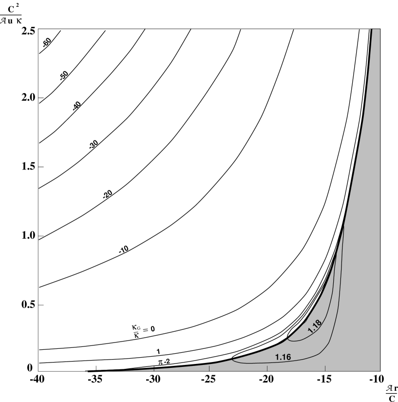
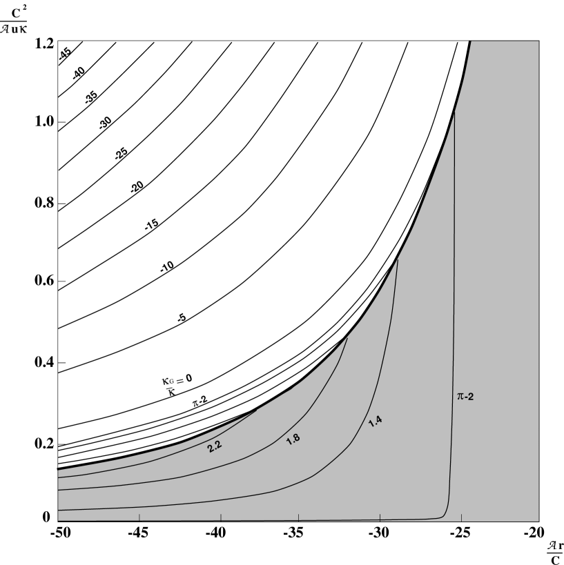
FIG. 10.: Phase diagram for constant area vesicles of genus zero or one, with intrinsic vector ($n=1$) order. The position of the transition line between genera depends on the ratio of intrinsic and total bending rigidities $\frac{\kappa_{G}}{\kappa}$. In the un-shaded region, genus one vesicles are axisymmetric, circular cross-section tori, whose aspect ratio is given in Fig(9). Genus one vesicles that exist in the shaded region are non-axisymmetric. The area of the diagram occupied by spherical vesicles decreases with increasing $\frac{\kappa_{G}}{\kappa}$.

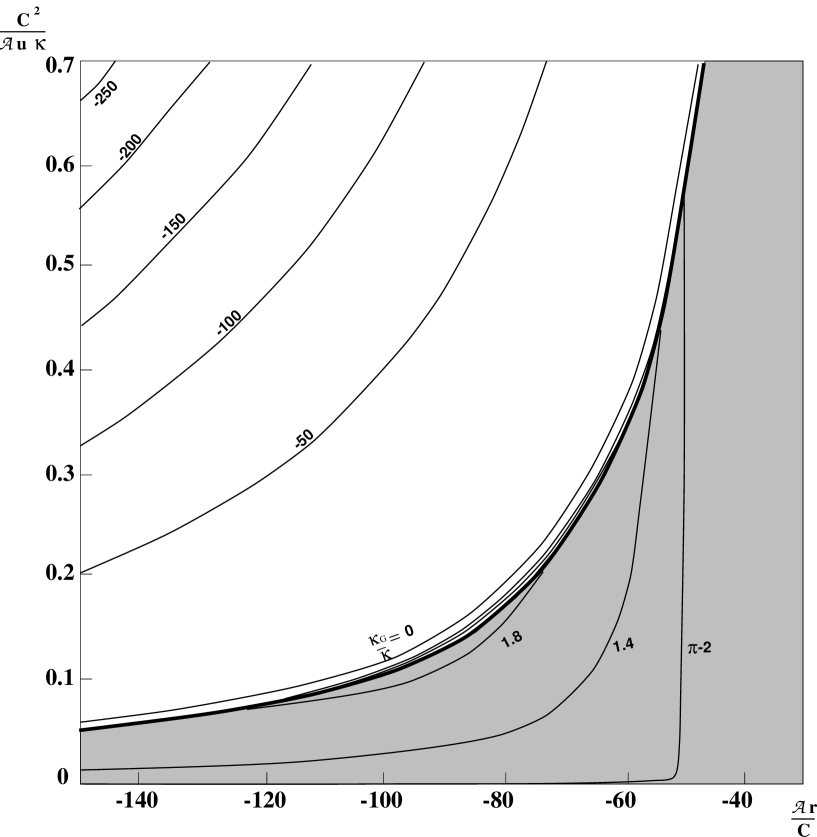
FIG. 11.: Phase diagram for constant area vesicles of genus zero or one, with intrinsic nematic ($n=2$) order.

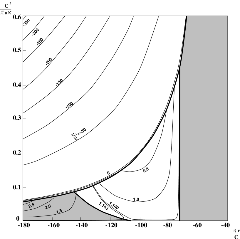
FIG. 12.: Phase diagram for constant area vesicles of genus zero or one, with intrinsic tetratic ($n=4$) order.

FIG. 13.: Phase diagram for constant area vesicles of genus zero or one, with intrinsic hexatic ($n=6$) order.

The $n^{S}_{n-1}$ phases do not persist when this larger phase space is explored, except for $6^{S}_{5}$, for which $\lambda_{0}$ is less than the sphere value of $6$, when $\alpha$ is close to $\sqrt{2}$. The diagrams are each divided into shaded and unshaded regions by a heavy line. In the shaded regions, vesicles are either spheres or non-axisymmetric tori while, in unshaded regions, either spheres or axisymmetric tori occur.

Consider first the $n=1$, $n=2$ and $n=4$ phase diagrams. A transition line, whose position depends on $\frac{\kappa_{G}}{\kappa}$ separates tori from spheres. Note that for $\frac{\kappa_{G}}{\kappa}>\pi-2$, the transition line is closed, with spheres on the inside and tori of one sort or another on the outside, while for $\frac{\kappa_{G}}{\kappa}<\pi-2$, the line is open, with spheres on the high-temperature side and axisymmetric tori on the low-temperature side. This magical value of $\pi-2$ is the critical value of $\frac{\kappa_{G}}{\kappa}$ at which spheres would become tori if the model described curvature energy alone and did not include terms in $\psi$. Note that in these three phase diagrams the separatrix (the $\frac{\kappa_{G}}{\kappa}=\pi-2$ transition) has a vertical limb at the value of $\frac{{\cal A}r}{C}$ at which ordering first forms on the sphere, ie. at $r=r_{c}^{\mbox{sphere}}$.

The $n=6$ diagram in Fig.(13) is a little more complicated since there are two distinct phases of ordering on axisymmetric tori. Again, the diagram is divided into shaded and unshaded regions. The shaded region is now split into two parts. The part on the right contains spheres if $\frac{\kappa_{G}}{\kappa}<\pi-2$, and non-axisymmetric tori otherwise. The part on the left contains spheres on the high $\frac{C^{2}}{{\cal A}u\kappa}$ side of the transition line (whose position depends, of course, on $\frac{\kappa_{G}}{\kappa}$) and non-axisymmetric tori on the other side. The un-shaded region, which contains axisymmetric tori and spheres, is also divided into two parts. The part in the top left of the diagram behaves as described above for the other phase diagrams. The other part may (depending on $\frac{\kappa_{G}}{\kappa}$) contain a closed transition line, which, unlike the other closed transition lines we have met, has spheres on the outside and axisymmetric tori, of small aspect ratio and $6_{5}^{S}$ field configuration, on the inside.

The four phase diagram of Figs.(13)-(13) may seem complicated but they are easily understood if one remembers that: a) they are several diagrams superimposed, and b) the regions in which spherical vesicles exist become smaller as $\kappa_{G}$ increases, since spheres have more intrinsic curvature than tori. Having established from these diagrams that an axisymmetric torus exists in a certain region, its aspect ratio may be found from Figs.(9)-(9).

It should be mentioned that the curves defining the edges of the shaded regions in Figs.(13)-(13) have been slightly smoothed by hand to remove pixcellation which arose from numerical rounding errors.

X Validity of the Approximations

Some order-of-magnitude calculations are now presented to give an indication of the regimes of validity of the various approximations used.

A Lowest Landau Level Approximation

The Landau levels form a complete set of orthogonal functions in which to expand the order parameter; $\psi=\sum_{p}a_{p}\phi_{p}$. Each eigenfunction $\phi_{p}$ has an eigenvalue $\lambda_{p}$ defined by Eqs.(9) and (11). The lowest Landau levels alone may be used if $a_{p}\ll a_{q}$ where $\lambda_{p}\neq\lambda_{q}=\lambda_{0}$. As an indicator of the region in which this is valid, let us calculate $<a_{p}^{*}a_{p}>$ for Gaussian fluctuations above the continuous transition, using the quadratic Hamiltonian

$${\cal H}=\sum_{p}(r-\gamma\lambda_{p})b_{p}^{*}b_{p}+{\cal O}(b^{4})$$ (30)

where $\gamma\equiv-\frac{4\pi C}{\cal A}$ and $b_{p}\equiv\sqrt{\frac{\cal A}{4\pi}}a_{p}$. The partition function is

$${\cal Z}=\int\exp\sum_{p}(\gamma\lambda_{p}-r)b_{p}^{*}b_{p}\>\prod_{p}db_{p}^{*}db_{p}.$$

Hence

$$<b_{p}^{*}b_{p}>=\frac{\pi}{r-\gamma\lambda_{p}}.$$

So for the lowest landau levels, $<b_{p}^{*}b_{p}>_{0}=\frac{\pi}{r-r_{c}}$ and for the next lowest level, $<b_{p}^{*}b_{p}>_{1}=\frac{\pi}{r-\gamma\lambda_{1}}$. Hence the ratio of correlators is

$${\cal R}\equiv\frac{<a_{p}^{*}a_{p}>_{1}}{<a_{p}^{*}a_{p}>_{0}}=\frac{<b_{p}^{*}b_{p}>_{1}}{<b_{p}^{*}b_{p}>_{0}}=\frac{x}{x+4\pi(\lambda_{1}-\lambda_{0})}$$

where $x=\frac{{\cal A}(r-r_{c})}{C}$ is the x-coordinate in the phase diagrams, measured with respect to the transition. We see that ${\cal R}$ is small, and hence the lowest Landau level approximation is good, when $|x|\tilde{<}4\pi(\lambda_{1}-\lambda_{0})$, the right hand side of which may be estimated from Fig.(3). For the Clifford torus, $(\lambda_{1}-\lambda_{0})\sim 0.5$ so the approximation is quantitatively accurate only within $\sim$3 of the transition, along the x-axis. However, Figs.(9)-(13) cover a much larger region than this, in order to clarify the qualitative features of the diagrams, for which the calculation at this level of approximation is a useful guide. It should be noted that, at ‘transitions’ from one lowest Landau level configuration to another, $(\lambda_{1}-\lambda_{0})\rightarrow 0$, so the approximation must break down here, as noted in section VII B. Also, in the large-$\alpha$ phases below the first-order transitions, $r_{c}$ is higher, so the system is far from the lowest Landau level regime. These phases are included in the diagrams in order to show the first-order transitions.

B Mean Field Theory

For this order-of-magnitude analysis, let us treat two parts of the free energy separately: first we will demand that fluctuations in the Helfrich Hamiltonian may be neglected in the absence of orientational order, then, within this fixed, non-fluctuating environment, it will be required that the terms in $\psi$ satisfy the Ginzburg criterion for the validity of mean-field theory.

In a simplistic calculation, good over only a short range, the Monge gauge is used to parameterize a locally horizontal surface, defining its z-coordinate as a function of x and y. Keeping terms of second order in z, and expanding z in plane-wave modes: $z\sim{\cal A}^{\frac{1}{2}}\sum_{k}c_{k}e^{ik\cdot x}$ gives

$$\kappa\int(K_{a}^{a})^{2}d{\cal A}\approx\kappa\int(\nabla^{2}z)^{2}dxdy=\kappa{\cal A}^{2}\sum_{k}|c_{k}|^{2}k^{4}.$$

Note that the Gaussian curvature energy does not influence fluctuations as it is a topological invariant. Hence

$$<|c_{k}|^{2}>=\frac{1}{\kappa{\cal A}^{2}k^{4}}$$

so, for fluctuations to be negligible on the scale of the system size requires $\kappa\gg\frac{1}{4\pi^{2}}$ . This is intuitively obvious; that a large bending rigidity is required to combat fluctuations. In fact, this simple calculation on a flatish surface is over-stringent, since intrinsic curvature, as exists in closed surfaces, reduces the size of fluctuations [10].

The Ginzburg criterion is now computed for the Ginzburg-Landau part of the free energy. This is a comparison between the size of the discontinuity in specific heat at the phase transition, calculated with mean-field theory, and the size of the divergence in specific heat due to Gaussian fluctuations. Close to the transition, $r$ goes approximately linearly with temperature $T$. Hence $(r-r_{c})=\rho(T-T_{c})$, where $T_{c}$ is the shifted mean-field transition temperature, and $\rho$ is some constant. From Eq.(26) it follows that the mean-field discontinuity in specific heat is

$$\Delta C=\frac{\rho^{2}T_{c}^{2}}{4\pi uJ}.$$

For simplicity, the specific heat of fluctuations is calculated for the sphere, above the phase transition. Using the quadratic form Eq.(30), and only the $(2n+1)$ lowest Landau levels, gives a free energy density $f=\frac{(2n+1)T}{\cal A}(\ln\rho(T-T_{c})-\ln\pi)$. Hence the singular part or the specific heat is

$$C_{\mbox{sing.}}=\frac{(2n+1)\rho}{{\cal A}(1-\frac{T}{T_{c}})^{2}},$$

giving a critical exponent $\alpha=2$ since we are in a zero dimensional $k$-space. The ratio of these two specific heats is

$$\frac{C_{\mbox{sing.}}}{\Delta C}=\left(\frac{\zeta}{1-\frac{T}{T_{c}}}\right)^{2}$$

where

$$\zeta=\sqrt{\frac{4\pi(2n+1)uJ}{{\cal A}\rho T_{c}}}$$

and mean field theory is good for $|r-r_{c}|\tilde{>}\zeta$ . (N.B. This condition is equivalent to demanding that tree graphs dominate over one-loop graphs.) So the threshold, in the phase diagrams, between the mean-field regime and the fluctuation-dominated regime is given by the curve $x^{2}y=(2n+1)/\kappa$, where $x\equiv\frac{{\cal A}(r-r_{c})}{C}$ and $y\equiv\frac{C^{2}}{{\cal A}u\kappa}$, having set $\rho\sim T_{c}^{-1}$ and $J\sim\frac{1}{4\pi}$. At a height $y_{0}$, this region has width $\Delta=\sqrt{\frac{4\pi(2n+1)J}{\kappa y_{0}}}$. This should be much smaller than the region of interest ie. that in which the lowest Landau level approximation is valid. So $\Delta\ll 3$ and, by inspection, in all the phase diagrams, we are interested in $y_{0}\sim\frac{1}{n}$. Consequently the condition for a mean-field treatment of the order parameter to be valid in this investigation is just $\kappa\gg\frac{n^{2}}{9}$, which is always consistent with the validity of a mean-field treatment of the membrane shape, calculated above.

C The Ginzburg-Landau Model

The Ginzburg-Landau free energy functional is and expansion in $\psi$, truncated at order $\psi^{4}$. This is valid when ${\cal A}|\psi|^{2}\ll 1$. In the mean-field regime, this is always the case above the continuous transition. Below the transition, $\psi\sim\frac{|r-r_{c}|}{uJ\sqrt{4\pi}}$, from Eq.(25). So the inequality is marginal when $y\sim\frac{C}{\pi{\cal A}\kappa x}$ where $x$ and $y$ are given above. This defines a region in the phase diagrams of width $\Delta=\frac{Cn}{\pi{\cal A}\kappa}$ at a height $y=\frac{1}{n}$, which is in the region of interest. Again, let’s demand that $\Delta>>3$ to be consistend with the region of validity of the lowest Landau level approximation. Consequently, it is required that $\frac{C}{\cal A}\gg\frac{3\pi}{n}\kappa$.

Dropping constants of order unity, we find that mean-field theory, the Ginzburg-Landau model and the lowest Landau level approximation are all valid in a region of half-width $\sim 3$ in the phase diagrams, given that

$$\frac{C}{\cal A}\gg\kappa\gg 1.$$

D The Shapes

Close to the ordering transition, $\psi$ is very small, so the order cannot deform the torus far from Clifford’s aspect ratio $\sqrt{2}$, or the genus-zero shape far from a sphere, so the vesicle shapes used in this theoretical investigation are undoubtedly good. As Park et al. discovered in [2], $\psi$ wants to live in a flat space, and can achieve a flattening of the membrane via the gauge-like coupling in Eq.(3). This it will do where it is large, at the expense of an increased curvature where $\psi$ is small eg. at the defects. This pay-off is unavoidable, since the integral of intrinsic curvature is topologically fixed. Hence spherical vesicles are slightly deformed by the in-plane order, into rounded polyhedra, whose vertices are at the order parameter’s vortices. This is the effect which has been ignored in this paper. The same process will also occur in tori, especially in those parts of the phase diagrams where ordering is predicted to deform the tori to large aspect ratios. In general, one might expect that the larger the aspect ratio, the worse the approximations of circular cross-section and axisymmetry. But nature is on our side here. Since, in these large-aspect-ratio tori, $\psi$ is always in the $n_{0}^{S}$ configuration, which has no vortices, and becomes very uniform for large aspect ratios. So, although this approximation results in some quantitative inaccuracies, they are likely to be small. Also, they must change the free energy of the torus and the sphere, if not by the same amount, then at least in the same direction. So the phase diagrams may not have exactly the right numbers, but they do have more-or-less the right shape.

XI Conclusion

It is clear that orientational order in a toroidal geometry is a subject rich in physical diversity, and deserving of further study in condensed matter theory. Also, introducing orientational order into the surface is an interesting way of stabilizing a torus against the massless Goldstone mode of conformal transformations, without resorting to spontaneous curvature or a constraint of constant volume or bilayer area difference. As far as experimental verification is concerned, the principal results of this paper are embodied in the final four phase diagrams. The approximations used in their derivation may result in quantitative inaccuracies, but the main qualitative features of these diagrams are predicted to be seen in experiment in the future. At present an experimental realization is somewhat difficult, due to the fragile nature of laboratory-produced vesicles.

XII Acknowledgements

I would like to thank Prof. Mike Moore for his guidance in this work. I am grateful for the helpful comments of Tom Lubensky, Udo Seifert, Renko de Vries and the numerous others with whom I have conversed on the subject. I wish to acknowledge the EPSRC for my funding.

A Table of Mean-Field Phase Transitions

The axisymmetric toroidal aspect ratios at which the order parameter field, which minimizes the free energy in the regime of the lowest Landau level approximation, changes its configuration between states of different $p$ or different symmetry are given in the table below. See sections VII B and VIII A for explanations of these transitions. Note that an $n=1$ (vector) field has no such transitions, as its ground state is always $1_{0}^{S}$.

Transition	Aspect Ratio
$2_{1}^{S}\rightarrow 2_{1}^{B}$	2.31
$2_{1}^{B}\rightarrow 2_{0}^{S}$	2.41
$4_{3}^{S}\rightarrow 4_{2}^{S}$	3.34
$4_{2}^{S}\rightarrow 4_{1}^{B}$	4.56
$4_{1}^{B}\rightarrow 4_{0}^{S}$	4.98
$6_{5}^{S}\rightarrow 6_{4}^{S}$	3.15
$6_{4}^{S}\rightarrow 6_{3}^{S}$	5.46
$6_{3}^{S}\rightarrow 6_{2}^{B}$	6.63
$6_{2}^{B}\rightarrow 6_{1}^{B}$	7.24
$6_{1}^{B}\rightarrow 6_{0}^{S}$	7.83

REFERENCES

- [1] F.C.MacKintosh and T.C.Lubensky, Phys.Rev.Lett. 67 1169 (1991).
- [2] Jeongman Park, T.C.Lubensky and F.C.MacKintosh, Europhys.Lett. 20,3 279 (1992).
- [3] D.E.Rutherford, Vector Methods (Oliver & Boyd Ltd., 1959).
- [4] Jeffrey R.Weeks, The Shape of Space (Marcel Dekker, 1985).
- [5] B.Fourcade, J.Phys.II France 2 1705 (1992).
- [6] F.Jülicher, U.Seifert and R.Lipowsky, J.Phys.II France 3 1681 (1993).
- [7] T.J.Willmore, Total Curvature in Riemannian Geometry, (Ellis Horwood Ltd., Chicester, 1982).
- [8] J.A.O’Neill and M.A.Moore, Phys.Rev.B 48 374 (1993).
- [9] F.David, Geometry and Field Theory of Random Surfaces and Membranes, in Statistical Mechanics of Membranes and Surfaces, ed. D.Nelson, T.Piran and S.Weinberg (World Scientific Publishing Co. Pte. Ltd., 1989)
- [10] R.de Vries, Private communication.