Mean-field transfer-matrix study of the magnetic phase diagram of CsNiF₃

Abstract

A method for treating ferromagnetic chains coupled with antiferromagnetic interactions on an hexagonal lattice is presented in this paper. The solution of the $1D$ part of the problem is obtained by classical transfer-matrix while the coupling between the chains is processed by mean-field theory. This method is applied with success to the phase diagram and angular dependence of the critical field of CsNiF₃. Results concerning the general influence of single-ion anisotropy on the magnetic ordering of such systems are also presented.

I introduction

Mean-field theory has long been a useful approximation for the study of phase transitions in a wide variety of systems, especially magnetic ones.[1] This comes from the great simplification of dealing with an averaged system instead of explicitely taking into account each individual interaction. As is generally the case, the interest here in using mean-field theory is its ability to predict phase transitions and to follow the evolution of relevant quantities close to the transition point. Unfortunately, transition points and critical exponents extracted from the mean-field theory are found to be significantly different from the experimental ones, especialy when the effective dimensionality is small. This is due to the averaging process involved which neglects the important critical fluctuations close to the transition point.

Although mean-field theory has some problems when applied directly to low dimensionality systems, it can be a very good approximation if used in conjunction with other techniques. By definition, quasi-one-dimensional (quasi-$1D$) systems have a direction in which the energy scale is much larger than in the others. Some numerical techniques such as classical transfer-matrix,[2, 3, 4, 5] quantum transfer-matrix,[6] and Bethe-Ansatz[7] can be used to solve almost exactly the $1D$ part of the problem and so, instead of using mean-field for all the interactions, it can be restricted to the coupling between the chains.[8] By doing this, important fluctuations, although not the critical ones, will be included and a more accurate solution can be expected.

The present work is mainly concerned with CsNiF₃ and, to some extent other equivalent systems. In this hexagonal insulator, the $S=1$ Ni²⁺ ions are ferromagnetically coupled in chains, along with the F^- ions. The chains are well separated from each other by large Cs⁺ ions and are coupled by antiferromagnetic interactions. This arrangment causes a large spacial anisotropy between the Ni ions, the ratio of the distance between these ions along the chains and in the basal plane being 0.4205, with an interchain separation of 6.27 $\mathaccent 28695{A}$. Anisotropy is thus present in the magnetic properties, the intrachain super-exchange ($J_{\parallel}=$ 20 K)[9] being much larger than the interchain one. The exact ratio between the super-exchange interactions is difficult to estimate because of the strong dipolar interaction arising between the ferromagnetic chains. It is important to note that dipolar field is almost nonexistant if the ordering along the chains is antiferromagnetic (AF), as it is in many other ABX₃ compouds such as CsMnBr₃ and CsNiCl₃.[10]

This strong dipolar field is responsible for the particular planar AF arrangement[11] of CsNiF₃ which is different from the expected 120^∘ structure of a system with only AF interactions on a triangular lattice. This magnetic phase occurs for temperatures smaller than $T_{N}\simeq 2.77$ K.[12]. Lussier et al.[12] have also shown a strong dependence of the critical field as a function of the angle between the magnetic field and the chain axis. As an example, at $T=2$ K, $H_{c\perp}\simeq 0.27$ T while for the other direction $H_{c\parallel}\simeq 2.3$ T. An unsuccesful attempt was made to fit this peculiar angular dependence of the critical field using a mean-field model similar to the one of Refs. [11] and [13]. In this paper, it will be shown that the experimental angular dependence is typical of a system formed by $XY$ ferromagnetic chains with AF coupling between them on a triangular lattice.

The Hamiltonian describing the magnetic properties of such systems is given by:

$${\cal H}=-J_{\parallel}\sum_{i}{\bf S}_{i}\cdot{\bf S}_{i+1}-J_{\perp}\sum_{<a,b>}{\bf S}_{a}\cdot{\bf S}_{b}-g\mu_{B}{\bf H}\cdot\sum_{i}{\bf S}_{i}+D\sum_{i}({\bf S}_{i})^{2}+{\cal H}_{Dipole}$$ (1)

The first, third and fourth sums in equation (1) are along the chain while the second one is between nearest neighbors in the plane perpendicular to the chains axis. The strong $XY$ behavior of CsNiF₃ comes from its large single-ion anisotropy ($D$) of 8.5 K.[9] The $g$-value was set to 2.2.

As mentioned previously, the usual mean-field theory uses averaged quantities for the three lattice dimensions. An example of this is found in Ref. [11]. The goal of the present work is to develop a method which treats the chains by classical tranfer-matrix and uses mean-field for the coupling between them. This method, refered to as MFTM (Mean-Field Transfer-Matrix), is presented in section II. It is followed, in Section III, by a brief review of the transfer-matrix algorithm used to calculate the magnetization and the susceptibility of a $1D$ chain as a function of temperature and magnetic field. In Section IV, MFTM is applied to CsNiF₃ for the calculation of its magnetic-field – temperature phase diagram and angular dependence of the critical field. Some other general results, concerning single-ion anisotropy, are presented in Section V.

II Mean-Field coupling of quasi-1D chains

Before presenting the calculated phase diagram of CsNiF₃, it is useful to understand qualitatively the underlying mecanism of the magnetic order in this system. For simplicity, consider a starting point below T_c with a magnetic field oriented in the $XY$ plane, large enough to destroy the AF order. In this phase, the paramagnetic one, the free-energy is dominated by a Zeeman term, $-{\bf m\cdot H}$, and the magnetization ${\bf m}$ is parallel to the applied field. As the field amplitude is lowered, this term is diminished up to a point where a perpendicular exchange term, proportional to $-J_{\perp}m^{2}$, becomes equal to it. At this field, since $J_{\perp}<0$, an AF order develops and a finite angle between the magnetic sub-lattices appears. The critical field, $H_{c}$, is defined where this angle is equal to zero. It is important to notice the particular planar structure of the magnetic order in CsNiF₃ (Fig. 1) which is different from the 120^∘ structure of CsMnBr₃, an $XY$ system having strong AF coupling along the chains. This difference is due to the relatively strong dipolar field originating from the neighboring ferromagnetic chains[11]. This dipolar field depends strongly on the angle between the magnetic sub-lattices and it can be shown quite easily that there is no interchain dipolar field present on a given site at $H_{c}$, where the magnetization of all the sub-lattices are parallel to the field. So, for small angles between the sub-lattices, the order starts to develop like a 120^∘ system (see Fig. 2) but at a given angle, the dipolar field coming from the other chains becomes large enough to flip one of the sub-lattices according to the planar arrangement of CsNiF₃ (Fig. 1).

The starting point of the theoretical description of such a system is the full three-dimensional ($3D$) Hamiltonian of equation (1). Since this Hamiltonian, applied to a triangular lattice, involves up to three magnetic sub-lattices, it is a highly non-trivial task to solve it even numerically. On the contrary, the one-dimensional ($1D$) part of the Hamiltonian consisting of first, third and fourth term can be calculated numerically quite easily and with good precision by the tranfer-matrix technique. The utility of mean-field theory for this problem comes from the fact that the $1D$ part has a much larger contribution to the free-energy ${\cal F}$ than the $3D$ one ($|J_{\parallel}|\gg|J_{\perp}|$).[8] Thermal averages of the $1D$ Hamiltonian can be used to approximate the free-energy of the $3D$ one. Formally, this type of free-energy is obtained using the Bogoliubov inequality:[14]

$${\cal F}\leq{\cal F}_{T}={\cal F}_{1D}+{\langle{\cal H-H_{\it 1D}}\rangle}_{1D}\ .$$ (2)

With the three magnetic sub-lattices of Fig. 2, and with a proper counting of each link in the $J_{\perp}$ term, this gives the following trial free-energy:

$${\cal F}_{T}={\cal F}_{1D} - J_{\perp}\sum_{i}(\ 3{\langle{\bf S}_{ia}\rangle}_{1D}\cdot{\langle{\bf S}_{ib}\rangle}_{1D}+3{\langle{\bf S}_{ia}\rangle}_{1D}\cdot{\langle{\bf S}_{ic}\rangle}_{1D}+3{\langle{\bf S}_{ib}\rangle}_{1D}\cdot{\langle{\bf S}_{ic}\rangle}_{1D})$$ (3)

$$- g\mu_{B}{\bf H}\cdot\sum_{i}({\langle{\bf S}_{ia}\rangle}_{1D}+{\langle{\bf S}_{ib}\rangle}_{1D}+{\langle{\bf S}_{ic}\rangle}_{1D})$$ (4)

The thermal averages $\sum_{i}\langle{\bf S}_{ia}\rangle$ are just the magnetisation ${\bf m}$ of the sublattice $a$. Using the angle definition of Fig. 2 for $\theta$ and defining $\phi$ as the angle between the field and the $XY$ plane, the trial free-energy can be written as:

$${\cal F}_{T}={\cal F}_{1D} - 3J_{\perp}\ (2\cos\theta+\cos 2\theta)m^{2}$$ (5)

$$- (1+2\cos\theta)\cos\phi Hm_{\perp}\ ,$$ (6)

where $m_{\perp}$ is the component of ${\bf m}$ in the $XY$ plane.

It is also important to note that equation (6) is valid only for small values of the angle $\theta$ where the dipolar field has no influence on the order. Minimising (6) with respect to $\theta$ gives $\sin\theta=0$ or,

$$\cos\theta={-1\over{2J_{\perp}}}\Bigl{[}{{\cos\phi Hm_{\perp}}\over{m^{2}}}+J_{\perp}\Bigr{]}\ .$$ (7)

This results is reasonable. At high fields, $\theta=0$, indicating the field-induced ferromagnetic (paramagnetic) phase. In zero field, and for a sufficiently low temperature, one gets the $120^{\circ}$ configuration. Of course, this type of structure is not applicable for CsNiF₃ but it reflects the ordering mecanism which is valid only for small values of $\theta$. As indicated above, $H_{c}$ is defined where $\cos\theta=1$ and it can be obtained by solving self-consistently the following equation:

$$-3J_{\perp}m^{2}=\cos\phi Hm_{\perp}$$ (8)

Each side of equation (8) represents a contribution to the free-energy ${\cal F}$ (to within a minus sign). The right-hand side is the magnetic field contribution $-{\bf m}\cdot{\bf H}$, the dominant one in the paramagnetic phase, while the left-hand is the $3D$ contribution of the ordered phase. Since ${\bf m}$ is bounded to unity, the field contribution will eventually dominate at high field and the phase with the lowest free-energy will be the paramagnetic one. The strength of the ordered phase is controlled by the parameter $J_{\perp}$. In some systems, like CsNiF₃, this parameter is not well known but it can be evaluated with this technique by fitting to experimental data.

From the limiting behavior of equation (8) at low field, it is also possible to calculate, within MFTM, the transition temperature in zero field,[8] $T_{c}$. This gives:

$$\chi_{1D}(T_{c},0)={{-1}\over{3J_{\perp}}}\ ,$$ (9)

where $\chi_{1D}$ is the $1D$ susceptibility. An interesting application of equation (9) is the possibility to calculate directly the value of $J_{\perp}$ needed for a given $T_{c}$. In the presents work, this is the only procedure used to set $J_{\perp}$.

The last item that needs to be solved in this mean-field theory is the value and the orientation of the external magnetic field ${\bf H}_{ext}$. Up to now, the field included in the calculation was the effective field applied to $1D$ chain. This is not the true external field; one needs to add a dipolar contribution ${\bf H}_{dip}$ and a $3D$ contribution, ${\bf H}_{3D}$, coming from the influence of the neighboring chains. Using ${\bf H}_{1D}$ to designate the field used previously in this paper this gives:

$${\bf H}_{ext}={\bf H}_{1D}-{\bf H}_{3D}-{\bf H}_{dip}\ .$$ (10)

Equation (10) is shown graphically in Fig. 3. This figure also shows two new angle definitions between fields and the $XY$ plane: $\theta_{ext}$ for ${\bf H}_{ext}$ and $\theta_{m}$ for ${\bf H}_{3D}$ and ${\bf H}_{dip}$. The evaluation of ${\bf H}_{3D}$ is straighforward it is just the number of near neighbors times $J_{\perp}$. It gives:

$${\bf H}_{3D}=6J_{\perp}{\bf m}$$ (11)

The dipolar field ${\bf H}_{dip}$ can be evaluated easily, if the magnetization of all the sub-lattices are parallel, since there is no interchain contribution. For ${\bf m}$ in the plane perpendicular to the chain this gives:

$${\bf H}_{dip}=-32.3K{\bf m}\ ,$$ (12)

with

$$K={{g^{2}\mu_{B}^{2}\mu_{o}}\over{4\pi a^{3}k_{B}}}\ .$$ (13)

Since CsNiF₃ has a quite strong $XY$ caracter, the component of ${\bf m}$ in the $XY$ plane was always by far the greatest for all the angles $\phi$ used in the calculation so that the numerical constant used in equation (12) was good to a few percent in all cases.

The fields ${\bf H}_{3D}$ and ${\bf H}_{dip}$ are important in evaluating the external field ${\bf H}_{ext}$ but they are not included in the calculation of $H_{c}$ by equation (8). The first one, ${\bf H}_{3D}$, is implicitely accounted for in the left-hand side of equation (8) while the second one, ${\bf H}_{dip}$, obviously turns with ${\bf m}$ so there is no free-energy changes due to it.

The phase transitions are obtained by the solution of equation (8) which implies a prior knowledge of ${\bf m}(T,H)$, the $1D$ magnetization. An effective and flexible way of calculating ${\bf m}$ is the transfer-matrix technique, which depends on the various $1D$ parameters like the single-ion anisotropy ($D$) and the parallel exchange interaction ($J_{\parallel}$).

III Transfer-Matrix technique

Since the present work relies heavily on the tranfer-matrix technique, a brief summary of this method is presented here. This study follows the work of Blume et al.[2] and assumes that the classical spin Hamiltonian for an $N$ spins chain of magnitude $S$ can be written as:

$${\cal H}_{s}=-\sum_{i=1}^{N}V(\hat{S}_{i},\hat{S}_{i+1}),$$ (14)

with

$$V(\hat{S}_{i},\hat{S}_{i+1})=\tilde{J}\hat{S}_{i}\cdot\hat{S}_{i+1}-{{\tilde{D}}\over 2}[(\hat{S}_{i}^{z})^{2}+(\hat{S}_{i+1}^{z})^{2}]+{{\tilde{\bf H}}\over 2}\cdot(\hat{S}_{i}+\hat{S}_{i+1})$$ (15)

and

$$\tilde{J}={{J_{\parallel}S(S+1)}\over{|J_{\parallel}S(S+1)|}}\ \ \ \Bigl{\{}{}^{\displaystyle\tilde{J}=1\Rightarrow F}_{\displaystyle\tilde{J}=-1\Rightarrow AF}$$ (16)

$$\tilde{D}={{DS(S+1)}\over{|J_{\parallel}S(S+1)|}}\ \ \ \Bigl{\{}{}^{\displaystyle\tilde{D}<0\Rightarrow Ising}_{\displaystyle\tilde{D}>0\Rightarrow XY}$$ (17)

$$\tilde{\bf H}={{g\mu_{B}{\bf H}\sqrt{S(S+1)}}\over{|J_{\parallel}S(S+1)|}}$$ (18)

$$\tilde{\beta}=\beta{|J_{\parallel}S(S+1)|}$$ (19)

The unit vectors $\hat{S}_{i}$ are oriented along the spin direction. Using these definitions, the partition function can be written[14] as a product of Boltzmann factors,

$$Z = \sum_{\{s_{i}\}}\exp\Bigl{[}\tilde{\beta}\sum^{N}_{i=1}V(\hat{S}_{i},\hat{S}_{i+1})\Bigr{]}$$ (20)

$$= \sum_{\{s_{i}\}}\prod_{i=1}^{N}\exp\Bigl{[}\tilde{\beta}V(\hat{S}_{i},\hat{S}_{i+1})\Bigr{]}\ .$$ (21)

Since $V$ is translationnaly invariant, the term in the product does not depend on the site chosen and $Z$ is given by:

$$Z={\rm Tr}K^{N}$$ (22)

with

$$K_{\mu\nu}\equiv\exp\Bigl{[}\tilde{\beta}V(\hat{S}_{i}^{\mu},\hat{S}_{i+1}^{\nu})\Bigr{]}$$ (23)

Since $N$ is a very large number, only the largest eigenvalue $\lambda_{0}$ of $K$ will contribute significantly to $Z$.

For classical spins, the transfer-operator $K$ needs to be mapped onto some discretisation of the spherical coordinates in order to evaluate it numerically. Following the procedure found in Ref. [5], which is suitable for broken rotational symmetry, one finds the $1D$ magnetization to given by:

$${\bf m}=\sum_{i=1}^{N_{\theta}}\sum_{j=i}^{N_{\phi}}W^{\theta}_{i}W^{\phi}_{j}\Psi_{0}(\theta_{i},\phi_{j})\Psi_{0}(\theta_{i},\phi_{j})[\cos(\theta_{i})\hat{z}+\sin(\theta_{i})\cos(\phi_{j})\hat{x}+\sin(\theta_{i})\sin(\phi_{j})\hat{y}],$$ (24)

where $\Psi_{0}$ is the eigenvector of $K$ corresponding to the largest eigenvalue $\lambda_{0}$ and, $N_{\theta}$, $N_{\phi}$, $W^{\theta}_{i}$, $W^{\phi}_{i}$, are respectively the number of coordinates and the Legendre weights of the discret spherical coordinates $\theta_{i}$ and $\phi_{i}$. In the absence of a magnetic field, or when the field is along the chain axis, a simplification using the rotational invariance of $V$ can be used.[4] The reduced number of coordinates for $K$ greatly improves the amount of computing time needed for a given precision. Such a simplification can be used to evaluate the susceptibility $\chi$ of the zero field equation (9). Using the results found in Ref. [2] the $1D$ susceptibility can written as:

$$\chi_{1D}^{zz}(q) = \tilde{\beta}\sum_{l=1}^{\infty}{{\lambda_{00}^{2}-\lambda_{l0}^{2}}\over{\lambda_{00}^{2}-2\lambda_{00}\lambda_{l0}\cos q+\lambda_{l0}^{2}}}\Bigr{[}\sum_{i=1}^{N_{\theta}}W^{\theta}_{i}\cos(\theta_{i})\Psi_{00}(\theta_{i})\Psi_{l0}(\theta_{i})\Bigl{]}^{2}$$ (25)

$$\chi_{1D}^{xx}(q) = {\tilde{\beta}\over 2}\sum_{l=1}^{\infty}{{\lambda_{00}^{2}-\lambda_{l1}^{2}}\over{\lambda_{00}^{2}-2\lambda_{00}\lambda_{l1}\cos q+\lambda_{l1}^{2}}}\Bigr{[}\sum_{i=1}^{N_{\theta}}W^{\theta}_{i}\cos(\theta_{i})\Psi_{00}(\theta_{i})\Psi_{l1}(\theta_{i})\Bigl{]}^{2}\ .$$ (26)

When using the rotational invariance as a simplification, one needs to introduce a second index in order to specify the azimuthal dependence. This second index is implicitely taken into account with the broken rotational symmetry algorithm. Typical matrix sizes are $28^{2}\times 28^{2}$ for the broken rotational symmetry algorithm while they are only $64\times 64$ for the rotational invariance one. In both cases the amount of computing is not excessive, ranging between seconds and minutes per $(T,H)$ point. Of course this figure increases rapidly with matrix size.

IV Application to CsNiF₃

The main goal of this work is to calculate the magnetic phase diagram of CsNiF₃. Figure 4 presents a comparison between the experimental phase diagram obtained with ultrasound by Lussier et al.[12] and the phase diagram calculated with the MFTM method. In this figure, the circles are the original experimental data and the squares are from the MFTM. The diamond at zero field is set to 2.77 K by an appropriate choice of $J_{\perp}$ according to equation (9). The value found for $J_{\perp}$ using this procedure is 0.0253 K. For this phase diagram and all the subsequent MFTM data on CsNiF₃ it will be the only value of $J_{\perp}$ used. The overall agreement between theory and experiment is good considering the fact that this mean-field theory neglects the $3D$ fluctuations which are not included in the transfer-matrix calculation and are the relevant ones close to $T_{c}$. It is quite obvious from the development of MFTM that $H_{c}$ scaled as ${\bf m}$ and so $H_{c}\sim(T_{N}-T)^{\beta}$. The absence of the $3D$ fluctuations thus reflects itself in the critical exponent $\beta$, giving the usual mean-field value of $1/2$ value for the theoretical phase diagram. This compares with an experimental estimate[12] of $\beta=0.31$.

The large $XY$ single-ion anisotropy in CsNiF₃ has an important effect on the angular dependence of $H_{c}$. Crudely, one can say that when increasing the field for $T\ll T_{c}$ the transition occurs when ${\bf m}$ saturates so that the left side of equation (8) becomes bounded and the $H$ term at the right can dominate. Because of the $XY$ anisotropy of CsNiF₃, ${\bf m}$ will grow rapidly along the projection of ${\bf H}$ in the $XY$ plane and it will saturate for approximately the same field for small angles of the field out of the plane. For large angles, the projection of ${\bf H}$ in the $XY$ plane will be small and ${\bf m}$ will grow more slowly giving a larger $H_{c}$. This type angular dependence is shown in Fig. 5. In this figure, the experimental data of Ref. [12] and the MFTM results are represented respectively by the circles and the diamond. The agreement, already quite good between these data, becomes excellent when a possible correction for a misalignement of the experimental plane of rotation of 6^∘ is included (circles). This correction, although large, is not unreasonable. One should also consider the nature of the theoretical method used as a source of error, especially close to $\theta=90$, a pathological angle for the present method since the coupling between ${\bf m}_{\perp}$ and $H$ then tends to zero. As mentioned earlier, even for the largest angle of the magnetic field out of the $XY$ plane used, ${\bf m}$ was always out the plane by less than 10^∘ so that the numerical constant in equation (12) was valid to a few percent. The good agreement found in Fig. 5 constrasts sharply with the failure of full $3D$ mean-field theory, as mentioned in Ref. [12].

V Single-ion Anisotropy

More generally, in the absence of a magnetic field, the paramagnetic phase transitions are determined by the magnetic susceptibility of the system according to equation (9). When a single-ion anisotropy is present, like in the Ising and $XY$ cases, the susceptibility is not isotropic and only the largest component needs to be taken into account. For an Ising system it is the longitudinal component $\chi_{1D}^{zz}(0)$ while for an $XY$ one, it is one of the transverse components $\chi_{1D}^{xx}(0)$ or $\chi_{1D}^{yy}(0)$. The equation (9) is particularily useful since from the knowledge of the susceptibility at a given temperature one can extract the perpendicular exchange interaction $J_{\perp}$ needed for a phase transition at this temperature. Such plots, for various values of $\tilde{D}$ in a system having $J_{\parallel}=1$ and $S=1$ are shown in Fig. 6. One can observe in this figure three limiting cases; the Heisenberg one at high values of $J_{\perp}$, the $XY$ one at intermediate values and the Ising one at low values. This can be easily understood, the general effect of the single-ion anisotropy is to favor the order by increasing the susceptibility when reducing the degrees of freedom of the spin system. It is especially true if the anisotropy is of the Ising type since the degrees of freedom become discrete. The $XY$ anistropy has a similar influence but it is less pronounced, the degrees of freedom being still continuous. Of course, at high enough temperature $(T\simeq D/k_{B})$ the Heisenberg behavior is recovered in all cases.

There is a functional difference between the continuous and discrete degrees of freedom. For the continuous ones, the low $J_{\perp}$ behavior is characterised by a power law of the from $T_{c}\sim J_{\perp}^{1/2}$. The dotted line, having a 1/2 slope, helps appreciate this. On the contrary, the discrete one (Ising) shows a more complex exponential form. These results are in agreement with the arguments of Villain et al.[15] Their result for the Ising case is shown by the dashed curve.

The last aspect investigated in this paper is the influence of the amplitude of the $XY$ single-ion anisotropy on the whole phase diagram. As seen in the previous paragraph an increase of the anisotropy will enhance the magnetic order as a function of the temperature by increasing the susceptibility. As a function of the magnetic field, for $T\ll T_{c}$, the anisotropy should have a much smaller effect since it is not implied directly in the phase transition. Figure 7 shows such phase diagrams for a magnetic field in the $XY$ plane and for three values of $\tilde{D}$; 0.1, 0.2 and 0.5. The value of $J_{\perp}$ has been set arbitrarily and the same lattice parameters than CsNiF₃ have been used. In zero field, the predicted behavior is observed, the highest $T_{c}$ being with $\tilde{D}=0.5$ while the lowest is with $\tilde{D}=0.1$. For a constant temperature smaller than $T_{c}$ (like $T/2J_{\parallel}=0.06$), one can also observe the small effect of $\tilde{D}$ on $H_{c}$.

VI Conclusion

In this work, a method for treating antiferromagnetically coupled ferromagnetic chains by mean-field theory has been developed for a system with a hexagonal lattice. The solution of the $1D$ part of the problem has been obtained by a generalised tranfer-matrix algorithm which is suitable for broken rotational symmetry.[5] Although special care has been needed to correctly account for the large dipolar field originating from the ferromagnetic chains, it has been possible to reproduce with succes the phase diagram of CsNiF₃ by only adjusting the value of $J_{\perp}$. The peculiar dependence of the critical field of CsNiF₃ as a function of the angle between the magnetic field and the chain axis has also been reproduced successfully,[12] in sharp contrast with $3D$ mean-field theory.

More generally, the dependence of the critical temperature as a function of $J_{\perp}$ has been established for various values of the single-ion anisotropy $D$. For the cases having continuous degrees of freedom, like the $XY$ and Heisenberg ones, a $T_{c}\sim J_{\perp}^{1/2}$ has been found while for the Ising case a more complex form has been obtained. These results are all in agreement with the ones obtained by Villain et al in Ref. [15]. For the $XY$ case, the effect of the size of the single-ion anisotropy on the overall shape of the phase diagram have also been investiguated. The results are in agreement with some simple physical arguments, an increase of $T_{c}$ with $D$ and a rather small effect on $H_{c}$ for temperatures much lower than $T_{c}$.

On the basis of the success of this method for the phase diagram of CsNiF₃, some extensions can be considered. The phase diagram of AF-chains compounds with $XY$ behavior, like CsMnBr₃,[10] could be examined although some complications with the transfer-matrix algorithm, coming from the difference in the effective field of the two staggered sub-lattices, are expected. Since successive phase transitions occur, the present method, based on linear response theory, must be generalized so that the free-energy itself is calculated.[16] A more challenging prospect is the application of this method to easy-axis AF chains systems like CsNiCl₃.[10] In this case, the single-ion anisotropy plays an active role in the magnetic ordering so it cannot be taken into account only by the transfer-matrix solution of the $1D$ part of the problem; it must also be included in the calculation $3D$ free-energy. This will add at least an order of magnitude to the complexity of the problem.

FIG. 1.: Planar arrangement of the two magnetic sub-lattices of CsNiF₃ for $H=0$ and $T<T_{c}$.

FIG. 2.: Ordering of a three antiferromagnetic sub-lattice system at a magnetic field close to $H_{c}$.

FIG. 3.: Vectorial construction giving ${\bf H}_{ext}$

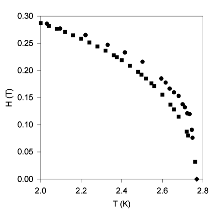
FIG. 4.: Comparison between the experimental phase diagram of CsNiF₃ given in Ref. [12] (circles) and the one calculated by the method described in this paper (squares). The diamond represent the zero field point used to set $J_{\perp}$ according to eqn. (9).

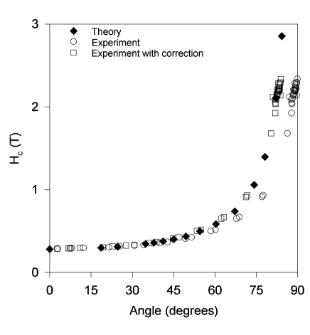
FIG. 5.: Comparison between the experimental angular dependence of $H_{c}$ at $T=2$ K given in Ref. [12] (circles and squares) and the one calculated by the method described in this paper (diamond). The squares represent the original data (circles) corrected for a plane of rotation misalignment of 6^∘.

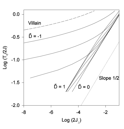
FIG. 6.: Logarithm of $T_{c}$ as a function of the logarithm of $2J_{\perp}$. The curves shown are for D=0, 0.001, 0.01, 0.1, 1, -0.01, -0.1, -1 and the Villain’s expression of Ref. ([15]).

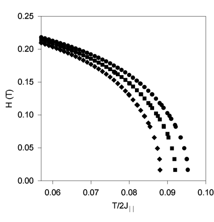
FIG. 7.: Magnetic phase diagrams for various D values; 0.5 (circles), 0.2 (squares) and 0.1 (diamond). The $J_{\perp}$ has been set arbitrarily.

- [1] H. Eugene Stanley, Introduction to phase transitions and critical phenomena, Oxford Science Publication, 79 (1971).
- [2] M. Blume, P. Heller and, N. A. Lurie, Phys. Rev. B11, 4483 (1975).
- [3] J. M. Loveluck, J. Phys. C, 12, 4251 (1979).
- [4] J.-G. Demers and A. Caillé, Solid State Comm. 68, 859 (1988).
- [5] Y. Trudeau, A. Caillé, M. Poirier, and J.-G. Demers Solid State Comm. 82, 825 (1992).
- [6] T. Delica and H. Leschke, Physica A 168, 736 (1990); T. Delica, W. J. M. de Jonge, K. Kopinga, H. Leschke and H. J. Mikeska, Phys. Rev. B44, 11 773 (1991).
- [7] M. Takahashi: Phys. Rev. B43 5788, (1991).
- [8] D. J. Scalapino, Y. Imry and P. Pincus, Phys. Rev. B11, 2042 (1975).
- [9] C. Dupas and J. P. Renard, J. Phys. C 10, 5057 (1977).
- [10] Magnetic Systems with Competing Interactions, edited by H. T. Diep, World Scientific, Singapour, (1994).
- [11] M. Scherer and Y. Barjhoux, Phys. Status Solidi B 80, 313 (1977). N. Suzuki, J. Phys. Soc. Jpn. 52 3199 (1983).M. L. Plumer and A. Caillé, Phys. Rev. B37, 7712 (1988).
- [12] B. Lussier and M. Poirier, Phys. Rev. B48,
- [13] M. Poirier, M. Castonguay, A. Caillé, M. L. Plumer and B. D. Gaulin, Physica B 165-166, 171 (1990).
- [14] J. J. Binney, N. J. Dowrick, A. J. Fisher, and M. E. J. Newman, The theory of critical phenomena, Oxford Science Publications, 61 (1992).
- [15] J. Villain and J. M. Loveluck, J. Phys. 38, L-77 (1977).
- [16] O. Heinonen, Phys. Rev. B47, 2661, (1993).